The R package sdcMicro serves as an easy-to-handle, object-oriented S4 class ... increasing since economic analysis or empirical analysis of the society is often ...
JSS
Journal of Statistical Software October 2015, Volume 67, Issue 4.
doi: 10.18637/jss.v067.i04
Statistical Disclosure Control for Micro-Data Using the R Package sdcMicro Matthias Templ
Alexander Kowarik
Bernhard Meindl
Vienna University of Technology
Statistics Austria
Statistics Austria
Abstract The demand for data from surveys, censuses or registers containing sensible information on people or enterprises has increased significantly over the last years. However, before data can be provided to the public or to researchers, confidentiality has to be respected for any data set possibly containing sensible information about individual units. Confidentiality can be achieved by applying statistical disclosure control (SDC) methods to the data in order to decrease the disclosure risk of data. The R package sdcMicro serves as an easy-to-handle, object-oriented S4 class implementation of SDC methods to evaluate and anonymize confidential micro-data sets. It includes all popular disclosure risk and perturbation methods. The package performs automated recalculation of frequency counts, individual and global risk measures, information loss and data utility statistics after each anonymization step. All methods are highly optimized in terms of computational costs to be able to work with large data sets. Reporting facilities that summarize the anonymization process can also be easily used by practitioners. We describe the package and demonstrate its functionality with a complex household survey test data set that has been distributed by the International Household Survey Network.
Keywords: confidentiality, micro-data, statistical disclosure control, R.
1. Introduction Statistical disclosure control (SDC) is an emerging field of research. More and more data on persons and establishments are collected by statistical organizations and almost all of these data holds confidential information. The demand for micro-data for researchers is increasing since economic analysis or empirical analysis of the society is often only possible by investigating data containing detailed information. In addition, also the demand for complex micro-data for training purposes seems to increase. Furthermore, public-use and
sdcMicro: Statistical Disclosure Control for Micro-Data in R
2 hhhh
µ-Argus Method 4.2 hhh h Frequency counts 4 Individual risk 4 Individual risk on households 4 l-diversity SUDA2 Global risk 4 Global risk with log-lin mod. Recoding 4 Local suppression (4) Swapping (4) PRAM 4 Adding correlated noise Micro-aggregation 4 Shuffling Utility measures (4) GUI (4) CLI Missing values 4 Cluster designs 4 Large data Reporting 4 Platform independent Free and open-source hhhh h
Software
hhhh
sdcMicro 1.0.0 (4) (4)
(4) (4) (4) 4 4 (4) 4 4
4 4
sdcMicro > 4.3.0 4 4 4 4 4 4 4 4 4 4 4 4 4 4 4 4 4 4 4 4 4 4
sdcMicroGUI > 1.1.0 4 4 4 4 4 4 4 4 4 4 4 4 4 4 4 4 4 4 4
IHSN 4 4 4 4 4 4 (4) (4) 4 4 4 4
4 4 4 (4) 4 4
Table 1: List of methods supported by different statistical disclosure control software. Ticks are in brackets when only limited support is provided to a method. A comparison to version 1.0.0 of sdcMicro (released May 29, 2007; published in Templ 2008) is given to indicate the progress of the new complete reimplementation of the package.
scientific-use files are required by researchers to run complex simulation studies to compare methods. As examples for such simulation studies, the BLUE-ETS, AMELI, DACSEIS and EUREDIT research projects from the Framework Programmes for Research of the European Union can be named. As examples for releases of public-use data sets, we mention data sets from the U.S. Census Bureau including the Current Population Survey, the Survey of Income and Program Participation, the American Housing Survey, the Survey of Program Dynamics, the American Community Survey and the Consumer Expenditure Survey (see, e.g., Task Force on the Conference of European Statisticians 2007). In any case, due to national laws on privacy, micro-data cannot be distributed to the public or to researchers whenever re-identification of persons or establishments is possible. Software packages are fundamental for the anonymization of data sets. Table 1 gives an overview on methods available in four software products – the µ-Argus software (Hundepool et al. 2008) from Statistics Netherlands, different versions and an extension of the R package sdcMicro (Templ, Kowarik, and Meindl 2015) and C++ code that was written by the International Household Survey Network (IHSN, see http://www.ihsn.org/home/node/32). For the sake
Journal of Statistical Software
3
of completeness, a former version of sdcMicro (Templ 2008) is also listed as well as the point and click graphical user interface sdcMicroGUI (Kowarik, Templ, Meindl, and Fonteneau 2013) that serves as an easy-to-handle, highly interactive tool for users who want to use the sdcMicro package but are not familiar with the native R command line interface. µArgus is a general tool for the anonymization of micro-data that has been developed by Statistics Netherlands with support from Eurostat and the 5th Framework Programme for Research of the European Union. sdcMicro version > 4.3.0 provides many more methods than µ-Argus and sdcMicro version 1.0.0, but major differences can also be found in the implementation. The main advantages of the proposed sdcMicro package consists of its userfriendly object-oriented application, the ease of importing data (in µ-Argus an import script which determines the hierarchical structure of data has to be written), its flexibility to use and the efficient implementation. We cannot compare computation speed of µ-Argus to sdcMicro, as methods cannot be applied using a command line interface, but we would like to point out that µ-Argus is not suitable for large data sets. It becomes slow and runs out-of-memory even with medium-sized data sets. This is also true for sdcMicro, version 1.0.0. This contribution is structured in the following manner. First the basic concepts to anonymize micro-data are briefly introduced in Section 2 and possible challenges related to large complex data sets are mentioned. A work flow shows how and when methods may be applied during the whole anonymization process. The conceptional difference regarding the distribution of the variables is underlined. In Section 3 the main functions of sdcMicro, their general usage and the object-oriented approach using S4 classes (Section 3.2) is explained. The next section, Section 4, gives more details about supported SDC methods. It starts with disclosure risk methods, followed by anonymization methods and methods to measure data utility. The application of the related sdcMicro functions is shown for each method. More precisely, the basic methods on measuring the disclosure risk of micro-data are explained in Section 4.1. Afterwards, a brief description of anonymization methods is given (Section 4.2). The measurement of data utility is included in Section 4.3. The reporting facilities are presented in Section 5. These reports summarize the whole anonymization applied to a defined object. Section 6 concludes with a summary of the main advantages of the package.
2. Concepts to anonymize micro-data A micro-data file is a data set that holds information collected on individual units like people, households or enterprises. In general, disclosure occurs when an intruder uses the released data to reveal previously unknown information about an individual.
2.1. Classification of variables For each unit/observation, a set of variables is recorded and available in the data set. These variables can be classified into groups, which are not necessarily disjunctive: Direct identifiers are variables that precisely identify statistical units. For example, social insurance numbers, names of companies or persons and addresses are direct identifiers. Key variables are a set of variables that, when considered together, can be used to identify individual units. For example, it may be possible to identify individuals by using a combination of variables such as gender, age, region and occupation. Key variables are
4
sdcMicro: Statistical Disclosure Control for Micro-Data in R also called implicit identifiers or quasi-identifiers. When discussing SDC methods, it is preferable to distinguish between categorical and continuous key variables based on the scale of the corresponding variables.
Non-confidential variables are variables that are not direct identifiers or key variables. For example, a variable containing information about the number of TVs in a household is non-confidential since this information is usually not available in any public data base and thus cannot be linked with auxiliary data. Sensitive variables are used for specific methods such as l-diversity (see Section 4.1). Information on cancer may serve as an example of a sensitive variable. Clustering variables are variables determining a hierarchical structure (e.g., households). Stratification variables are variables determining the application of methods on data subsets. Classification variables, such as economic branches, often serve as stratification variables and specific methods are then applied to each economic branch separately. The goal of anonymizing micro-data is to prevent confidential information from being assigned to a specific respondent. If linkage based on a number of identifiers is successful, the intruder has access to all of the information related to a specific corresponding unit in the released data. This means that a subset of critical variables can be exploited to disclose everything about a unit in the data set.
2.2. Challenges Methods used in statistical disclosure control borrow techniques from other fields. Multivariate methods are used to modify or simulate continuous variables (see, e.g., Muralidhar and Sarathy 2006; Templ and Meindl 2008b) and to quantify information loss (see, e.g., DomingoFerrer and Torra 2001) while distribution-fitting methods are used to quantify disclosure risks (see, e.g., Skinner and Holmes 1998; Franconi and Polettini 2004; Rinott and Shlomo 2006). Statistical modeling methods form the basis of perturbation algorithms (see, e.g., Muralidhar and Sarathy 2006), to simulate data (see, e.g., Drechsler 2011; Alfons, Kraft, Templ, and Filzmoser 2011) and to quantify risks and information loss (see, e.g., Shlomo 2010). Optimization methods may be used to modify data with a minimum impact on data quality (see, e.g., Fischetti and Salazar-González 2000). Large data sets present unique problems and challenges and place an even higher demand on computational efficiency. Handling missing values and structural zeros can be particularly challenging. Complex data structures, like those that are common in survey research, compound these challenges. SDC techniques can be divided into three broad topics: • measuring disclosure risk (see Section 4.1); • application of SDC-methods to deal with disclosure risks (see Section 4.2); • comparing original and modified data (information loss) (see Section 4.3).
Journal of Statistical Software
5
Figure 1: Possible work flow to anonymize micro-data using various SDC methods. The numbers 1–5 correspond to the enumerated explanations in Section 2.3.
2.3. Work flow Figure 1 outlines common tasks, practices and steps required to obtain confidential data. The following steps to perturbate micro-data are included in Figure 1: 1. The first step is to remove all direct identification variables from the micro-data set. 2. Second, a set of key variables used for all further risk calculations has to be selected. This decision is subjective and involves discussions with subject matter specialists and interpretation of related national laws. See Templ, Kowarik, and Meindl (2014) for practical applications. For the simulation of fully synthetic data, choosing key variables is not necessary, see for example Alfons et al. (2011). 3. After key variables have been selected, disclosure risks of individual units are measured. This step includes the analysis of sample frequency counts as well as the application of probability methods to estimate individual re-identification risks by taking population frequencies into account. 4. Next, observations with high individual risks are modified. Techniques such as recoding and local suppression, recoding and swapping or PRAM (post randomization method Gouweleeuw, Kooiman, Willenborg, and De Wolf 1998) can be applied to categorical key variables. It is possible to apply PRAM or swapping without recoding of key variables beforehand. However, lower swapping rates might be possible if key variables are modified in advance. The decision as to which method to apply also depends on the structure of the key variables. In general, one can use recoding together with local suppression if the amount of unique combinations of key variables is low. PRAM should be used if the number of key variables is large and the number of unique combinations is high; for details, see Sections 4.2 and 4.2 and for practical applications Templ et al.
6
sdcMicro: Statistical Disclosure Control for Micro-Data in R (2014). The values of continuously scaled key variables must be perturbed as well. In this case, micro-aggregation is always a good choice (see Section 4.2). More sophisticated methods such as shuffling (see Section 4.2) often also provide promising results. 5. After modifying categorical and continuous key variables, information loss and disclosure risk measures are estimated. The goal is to release a safe data set with low (individual) risks and high data utility. If the risks are low enough and the data utility is high, the anonymized data set can be released. If not, the entire anonymization process must be reiterated, either with additional perturbations if (some) remaining risks are considered too high or with actions that increase data utility.
Note that other concepts to anonymize micro-data such as the simulation of synthetic microdata sets exist (see Figure 1). One possibility is to simulate all variables of a micro-data set (i.e., simulate fully synthetic data) by statistical modeling and drawing from predictive distributions. This topic and its application in R is fully covered in Alfons et al. (2011) and Templ and Filzmoser (2014) and can be practically carried out using R package simPopulation (Alfons and Kraft 2013).
3. Working with sdcMicro For each method discussed we additionally show its usage via the command line interface of sdcMicro. The application of (most) methods is also possible using the graphical user interface of package sdcMicroGUI, but this is not shown in this contribution.
3.1. General information about sdcMicro and performance The first version, version 1.0.0, of the sdcMicro package was released in 2007 on the Comprehensive R Archive Network (CRAN, http://CRAN.R-project.org/package=sdcMicro) and introduced in Templ (2008). However, this version only included few methods and the package consisted of a collection of some functions that were only applicable to small data sets. The current release, version 4.6.0, is a huge step forward. Almost all methods are implemented in an object-oriented manner (using S4 classes) and have an internal implementation in C++ or based on package data.table (Dowle and Short 2013). This allows for efficient high performance computations. The IHSN provided C++ code for many methods which were rewritten from scratch (except suda2 and rankSwap) and integrated into sdcMicro. In Figure 2 the performance improvement with respect to computation time using the current version of sdcMicro (4.6.0) as compared to the previous implementation in version 4.0.4 using IHSN C++ code is shown. Note that these calculations are not possible for early versions of sdcMicro (Templ 2008) due to missing functionalities. To measure the computation time, a close-to-reality data set on household income and expenditures with 4580 observations on 14 variables was used. This data set is available in sdcMicro (?testdata). The observations were randomly replicated to enlarge the data set up to 10,000,000 observations. For different numbers of observations, frequency counts and risk (left plot in Figure 2) as well as (heuristic “optimal”) local suppression (right plot in Figure 2) were applied independently to each data set. While the IHSN C++ solutions has an exponentional increase in computation time with respect to the number of observations, the new implementation features a “linear growth” for local suppression. The computation time for 10,000,000 observations on four key variables is
Journal of Statistical Software
frequency estimation + risk measurement
7
optimal local suppression ● ●
● ●
500
400 400 ● ●
● ● ● ●
method
● IHSN C++ ●
● sdcMicro 4.1.0 ●
● ●
200
time in seconds
time in seconds
300 300 method ● IHSN C++ ● ● sdcMicro 4.1.0 ●
● ●
● ●
200
● ●
● ●
● ●
● ●
100
100
● ●
● ● ● ●
● ●
0
● ● ● ● ● ● ● ● ● ● ●● ● ● ● ● ●
0
0 2,500,000
5,000,000
7,500,000
number of observations
10,000,000
● ● ● ● ● ● ● ● ●● ● ● ● ● ● ● ● ●
0
2,500,000
5,000,000
7,500,000
10,000,000
number of observations
Figure 2: Computation time of IHSN C++ code (equals sdcMicro version < 4.1.0) and sdcMicro (version ≥ 4.1.0). approx. 500 seconds with any version of sdcMicro ≥ 4.1.0. On the other hand, with previous versions it is already out of scope to estimate the risk and apply local suppression for data sets with about 500,000 observations.
3.2. S4 class structure The following list gives an overview about the general aims of sdcMicro: • sdcMicro includes the most comprehensive collection of micro-data protection methods; • the well-defined S4 class implementation provides a user-friendly implementation and makes it easy to exploit its functionalities using sdcMicroGUI; • utility functions extract information from well-defined S4 class objects; • certain slots are automatically updated after application of a method; • an undo function allows to return to a previous state of the anonymization process without the need to do additional calculations; • for performance reasons, the methods are internally implemented either in C++ or by using the data.table package (Dowle and Short 2013); • dynamic reports about results of the anonymization process can be generated. To define an object of class ‘sdcMicroObj’, the function createSdcObj() can be used. Parameters for this function are for example categorical and continuous key variables, the vector of sampling weights and optionally stratification and cluster IDs. The following code shows how to generate such an object using a test data set of the International Income Distribution
sdcMicro: Statistical Disclosure Control for Micro-Data in R
8
Data Set (I2D2), which is distributed over the International Household Survey Network and which is also included in sdcMicro. R> library("sdcMicro") R. data("testdata", package = "sdcMicro") R> sdc slotNames(sdc) [1] [4] [7] [10] [13] [16] [19] [22]
"origData" "numVars" "strataVar" "manipPramVars" "originalRisk" "pram" "additionalResults" "deletedVars"
"keyVars" "weightVar" "sensibleVar" "manipNumVars" "risk" "localSuppression" "set"
"pramVars" "hhId" "manipKeyVars" "manipStrataVar" "utility" "options" "prev"
Slot origData contains the original data, keyVars the index of categorical key variables. pramVars contains an index indicating variables that are pramed (see Section 4.2 for details), slot numVars specifies indices of continuous key variables and the vector defining sampling weights is contained in slot weightVar. A possible index determining the cluster variable (slot hhId), the stratification variable (slot strataVar) and sensible variables (slot sensibleVar) can also be used. In addition, manipulated variables are saved in the slots beginning with manip. All risk measures (see Section 4.1) are stored in slots originalRisk (for the original unmodified data) and risk (for the manipulated data). Slot utility collects all information on data utility; further information on pramed variables and local suppressions are stored in slots pram and localSuppression while additional results (e.g., self-defined utility measures) are saved in slot additionalResults. Optionally, in the slot prev previous results are saved. Wrapper functions to extract relevant information from the ‘sdcMicroObj’ object are available (see Section 3.3). For more details on the structure of the ‘sdcMicroObj’ object have a look at the help file (help("createSdcObj")). The show (print) method shows some basic properties of objects of class ‘sdcMicroObj’: R> sdc Data set with 4580 rows and 14 columns. Weight variable: sampling_weight Categorical key variables: urbrur, water, sex, age
Journal of Statistical Software
9
Reported is the number | mean size and | size of smallest category ------------urbrur .. 2 | 2290 | 646 ------------water ... 8 | 572 | 26 ------------sex ..... 2 | 2290 | 2284 ------------age ..... 88 | 52 | 1 Number of observations violating - 2-anonymity: 330 - 3-anonymity: 674 -------------------------Percentage of observations violating - 2-anonymity: 7.21 % - 3-anonymity: 14.72 % Numerical key variables: expend, income, savings Disclosure Risk is between: [0% ; 100%] (current) - Information Loss: IL1: 0 - Difference Eigenvalues: 0 % Methods are applied to the ‘sdcMicroObj’ object and all related computations are done automatically. E.g., individual risks are re-estimated whenever a protection method is applied and the related slots of the ‘sdcMicroObj’ object are updated. A method for an ‘sdcMicroObj’ object can be applied by method(sdcMicroObj), where method is a placeholder for a specific method sdcMicroObj for an object of class ‘sdcMicroObj’. We note that sdcMicro also supports the straightforward application of methods to micro-data. For example, microaggregation of three continuous key variables (expend, income and savings) on the data set testdata can be achieved with: R> microaggregation(testdata[, c("expend", "income", "savings")]) This code is equivalent to microaggregation(sdc) where sdc is a ‘sdcMicroObj’ object and the three variables defined as numeric variables in slot numVars. In Table 2 we list the package’s current methods, function calls, function description, and slots updated in the ‘sdcMicroObj’ object by each method. For example, the application of localSuppression() on an ‘sdcMicroObj’ object suppresses certain values in the data set and afterwards it updates the slots risk and localSuppression. In the slot risk all relevant list elements are replaced
10
sdcMicro: Statistical Disclosure Control for Micro-Data in R
Function freqCalc()
Aim sample and population frequency estimation (used by measureRisk()) suda2() frequency calculation on subsets ldiversity() l-diversity measureRisk() individual, household and global risk estimation LLmodGlobalRisk() global risk estimation using loglinear models dRisk() disclosure risk for continuous scaled variables dRiskRMD() advanced disclosure risk measures for continuous scaled variables dUtility() data utility measures globalRecode() anonymization of categorical key variables groupVars() anonymization of categorical key variables localSupp() univariate local suppression of high risky values localSuppression()local suppression to achieve kanonymity pram() swapping values using the post randomization method microaggrGower() micro-aggregation on categorical and continuous key variables topBottomCoding() top and bottom coding addNoise()
perturbation of continuous variables rankSwapp() perturbation of continuous variables mafast() perturbation of continuous variables microaggregation()perturbation of continuous variables, wrapper for various methods shuffle() perturbation of continuous variables
Updates the slots –
@risk$suda2 @risk$ldiversity @risk* @risk$model @risk$numeric @risk$numericRMD (risk on cont. variables) @utility$* @risk$*, @manipKeyVars, @prev @risk$*, @manipKeyVars, @prev @risk$*, @localSuppression, @manipKeyVars, @prev @risk$*, @localSuppression, @manipKeyVars, @prev @pram, @manipPramVars, @prev @risk$*, @manipNumVars, @risk$*, @manipNumVars, @risk$numeric @manipNumVars, @risk$numeric @manipNumVars, @risk$numeric @manipNumVars, @risk$numeric @manipNumVars,
@utility$*, @prev @utility$*, @prev ), @utility$*, @prev ), @utility$*, @prev , @utility$*, @prev , @utility$*, @prev
@risk$numeric, @utility$*, @manipNumVars, @prev
Table 2: Functions in sdcMicro including various SDC methods. with new estimates and in the slot localSuppression the information of suppressed values gets updated. Another example is to apply microaggregation. R> sdc R> R> R>
ut R> R> R> R>
print(sdc) print(sdc, print(sdc, print(sdc, print(sdc, print(sdc,
"ls") type = type = type = type =
"recode") "risk") "numrisk") "pram")
More information on sdcMicro and its facilities can be found in the manual of sdcMicro, see Templ et al. (2015). The development version is hosted on https://github.com/alexkowa/ sdcMicro and includes test batteries to ensure that the package keeps stable when modifying parts of the package. From time to time, a new version is uploaded to CRAN.
Journal of Statistical Software
13
4. Methods In this chapter, a brief review of methods for statistical disclosure control is given. First, different kinds of disclosure risk methods are briefly discussed in Section 4.1 followed by a discussion on anonymization methods in Section 4.2. Concepts of data utility are briefly described in Section 4.3. More in-depth reviews of the procedures mentioned can be found, e.g., in Skinner (2009); Matthews and Harel (2011).
4.1. Measuring the disclosure risk Measuring risk in micro-data is a key task and is essential to determine if the data set is secure enough to be released. To assess disclosure risks, realistic assumptions about the information data users might have at hand to match against the micro-data set must be made. These assumptions are denoted disclosure risk scenarios. Based on a specific disclosure risk scenario, a set of key variables (i.e., identifying variables) must be defined that are used as input for the risk evaluation procedure. Based on these key variables, the frequencies of combinations of categories in the key variables are calculated for the sample data and are also estimated on population level. In the following, we focus on the analysis of these frequencies. Some methods only take available frequencies in the sample into account (k-anonymity, l-diversity, SUDA2). More sophisticated methods estimate the risk on estimated/modeled population frequency counts (individual risk approach, log-linear model approach). In any case it is the goal to obtain information on the risk for each individual unit and to summarize it to a global risk measure which evaluates the disclosure risk of the entire data set. Also, different methods can be applied to continuous key variables. These methods focus on the evaluation if perturbed (masked) values are too close to the original values.
Population frequencies and the individual risk approach Typically, risk evaluation is based on the concept of uniqueness in the sample and/or in the population. The focus is on individual units that possess rare combinations of selected key variables. It is assumed that units having rare combinations of key variables can be more easily identified and thus have a higher risk of re-identification. It is possible to crosstabulate all identifying variables and view their cast. Keys possessed by only few individuals are considered risky, especially if these observations also show small sampling weights. This means that the expected number of individuals having such keys is also expected to be low in the population. To assess if a unit is at risk, a threshold approach is typically used. If the re-identification risk of a unit is above a certain value, this unit is said to be at risk. To compute individual risks, the frequency of a given key pattern in the population must be estimated. To illustrate this approach, we consider a random sample of size n drawn from a finite population of size N . Let πj , j = 1, . . . , N be the (first order) inclusion probabilities. πj is the probability that element uj of a population of the size N is chosen in a sample of size n. All possible combinations of categories in the key variables (i.e., keys or patterns) can be calculated by cross-tabulating these variables. Let M be the number of unique keys. For each key, the frequency of observations with the corresponding pattern can be calculated, which results in M frequency counts. Each observation corresponds to one pattern and
sdcMicro: Statistical Disclosure Control for Micro-Data in R
14
the frequency of this pattern. Denote fi , i = 1, . . . , n to be the sample frequency count and let Fi be the population frequency count corresponding to the same pattern for the ith observation. If fi = 1 applies, the corresponding observation is unique in the sample given the key variables. If Fi = 1, then the observation is unique in the population and the sample. We note, that Fi is usually not known and has to be estimated. A very basic approach to estimate Fi would be to sum up the sampling weights for observations belonging to the same combination of key variables because the weights contain the information on expected units in the population. More sophisticated methods estimate these frequencies based on (log-linear) models, as discussed in a subsequent paragraph. In the following the methods are applied to the test data set. Before starting, the undolast() function is used to undo the last action (micro-aggregation applied in Section 3.2) R> sdc head(get.sdcMicroObj(sdc, type = "risk")$individual)
[1,] [2,] [3,] [4,] [5,] [6,]
risk fk Fk hier_risk 0.0016638935 7 700 0.004330996 0.0016638935 7 700 0.004330996 0.0005552471 19 1900 0.004330996 0.0004543389 23 2300 0.004330996 0.0024937656 5 500 0.009682082 0.0033222591 4 400 0.009682082
Without creating an object of class ‘sdcMicroObj’, one can use the function freqCalc() for frequency estimation. It basically includes three parameters (for benchmarking issues a fourth parameter is provided) determining the data set, the key variables and the vector of sampling weights (for details, see ?freqCalc). However, it can be shown that risk measures based on such estimated population frequency counts almost always overestimate small population frequency counts (see, e.g., Templ and Meindl 2010, and Section 4.1).
The concept of k-anonymity Based on a set of key variables, a desired characteristic of a protected micro-data set is often to achieve k-anonymity (Samarati and Sweeney 1998; Sweeney 2002). This means that for each possible key at least k units in the data set are assigned. This is equal to fi ≥ k, i = 1, . . . , n. A typical value is k = 3. The default print method of an object of class ‘sdcMicroObj’ can be used to see if the current ‘sdcMicroObj’ object already features 2- or 3-anonymity: R> print(sdc) Number of observations violating
Journal of Statistical Software
1 2 3 4 5 6
Key 1 1 1 1 1 2 2
Key 2 1 1 1 2 2 2
Sensible variable 50 50 42 42 62 62
fk 3 3 3 1 2 2
15 l-diversity 2 2 2 1 1 1
Table 4: k-anonymity and l-diversity on a toy data set. - 2-anonymity: 330 - 3-anonymity: 674 -------------------------Percentage of observations violating - 2-anonymity: 7.21 % - 3-anonymity: 14.72 % k-anonymity is typically achieved by recoding categorical key variables into fewer categories and by suppressing specific values of key variables for some units (see Sections 4.2 and 4.2).
l-diversity An extension of k-anonymity is l-diversity (Machanavajjhala, Kifer, Gehrke, and Venkitasubramaniam 2007). Consider a group of observations with the same pattern in the key variables and let the group fulfill k-anonymity. A data intruder can therefore by definition not identify an individual within this group. If, however, all observations have the same entries in an additional sensitive variable (e.g., cancer in the variable medical diagnosis), an attack will be successful if the attacker can identify at least one individual of the group, as the attacker knows that this individual has cancer with certainty. The distribution of the target-sensitive variable is referred to as l-diversity. Table 4 considers a small example data set that shows the calculation of l-diversity and points out the slight difference of this measure as compared to k-anonymity. The first two columns of Table 4 contain the categorical key variables. The third column of the data defines a variable containing sensitive information. Sample frequency counts fi appear in the fourth column. They equal 3 for the first three observations; the fourth observation is unique and frequency counts fi are 2 for the last two observations. Only the fourth observation violates 2-anonymity. Looking closer at the first three observations, we see that only two different values are present in the sensitive variable. Thus the l-(distinct) diversity is just 2. For the last two observations, 2-anonymity is achieved, but the intruder still knows the exact information of the sensitive variable. For these observations, the l-diversity measure is 1, indicating that sensitive information can be disclosed since the value of the sensitive variable equals 62 for both of these observations. Differences in values of the sensitive variable can be measured differently. We present here the distinct diversity that counts how many different values exist within a pattern/key. The l-diversity measure is automatically measured in sdcMicro for (and stored in) objects of class ‘sdcMicroObj’ as soon as a sensible variable is specified (using createSdcObj). Note that
16
sdcMicro: Statistical Disclosure Control for Micro-Data in R
the measure can be calculated at any time using ldiversity(sdc) with optional function parameters to select another sensible variable, see ?ldiversity. However, it can also be applied to data frames, where key variables (argument keyVars) and the sensitive variables (argument ldiv_index) must be specified as shown below: R> res1 print(res1) -------------------------L-Diversity Measures -------------------------Min. 1st Qu. Median Mean 3rd Qu. 1.00 4.00 8.00 10.85 17.00
Max. 35.00
Additional methods such as entropy, recursive and multi-recursive measures of l-diversity are also implemented. For more information, see the help files of sdcMicro.
Sample frequencies on subsets: SUDA2 SUDA (i.e., special uniques detection algorithm) estimates disclosure risks for each unit. SUDA2 (Manning, Haglin, and Keane 2008) is a recursive algorithm to find minimal sample uniques. The algorithm generates all possible variable subsets of selected (categorical) key variables and scans for unique patterns within subsets of these variables. The risk of an observation finally depends on two aspects: (a) The lower the number of variables needed to receive uniqueness, the higher the risk (and the higher the SUDA score) of the corresponding observation. (b) The larger the number of minimal sample uniqueness contained within an observation, the higher the risk of this observation. Item (a) is calculated for each observation i by li = m−1 k=MSUmin i (m − k), i = 1, . . . , n. In this formula, m corresponds to the depth, which is the maximum size of variable subsets of the key variables, MSUmin i is the number of minimal sample uniques (MSU) of observation i and n is the number of observations in the data set. Since each observation is treated independently, the specific values li belonging to a specific pattern are summed up. This results in a common SUDA score for all observations having this pattern; this summation is the contribution of Item (b). Q
The final SUDA score is calculated by normalizing these SUDA scores by dividing them by p!, with p being the number of key variables. To receive the so-called data intrusion simulation (DIS) score, loosely speaking, an iterative algorithm based on sampling of the data and matching of subsets of the sampled data with the original data is applied. This algorithm calculates the probabilities of correct matches given unique matches. It is, however, out of scope to precisely describe this algorithm here, see Elliot (2000) for details. The DIS SUDA score is calculated from the SUDA and DIS scores and is available in sdcMicro as disScore. Note that this method does not consider population frequencies in general, but considers sample frequencies on subsets. The DIS SUDA scores approximate uniqueness by
Journal of Statistical Software
17
simulation based on the sample information population but – to our knowledge – generally do not consider sampling weights. Thus, biased estimates may result. SUDA2 is implemented in sdcMicro as function suda2() based on C++ code from the IHSN. Additional output, such as the contribution percentages of each variable to the score, are also available as an output of this function. The contribution to the SUDA score is calculated by assessing how often a category of a key variable contributes to the score. After an object of class ‘sdcMicroObj’ has been created, no information about SUDA (DIS) scores are stored. However, after applying SUDA on such an object, they are available, see the following code where also the print method is used: R> sdc get.sdcMicroObj(sdc, type = "risk")$suda Dis suda scores table: - - - - - - - - - - thresholds number 1 > 0 4330 2 > 0.1 250 3 > 0.2 0 4 > 0.3 0 5 > 0.4 0 6 > 0.5 0 7 > 0.6 0 8 > 0.7 0 - - - - - - - - - - The individual SUDA scores and DIS scores are accessible in slots risk$suda2$score and risk$suda2$disScore as well as the contribution of each key variable to the SUDA score for each observation in slot risk$suda2$contributionPercent.
The individual and cluster risk approach An approach that considers sampling weights is the individual risk approach. It uses so-called super-population models. In such models population frequency counts are modeled given a certain distribution. The estimation procedure of sample counts given the population counts can be modeled for example by assuming a negative binomial distribution (see Rinott and Shlomo 2006) and is implemented in sdcMicro in function measure_risk() (for details, see Templ and Meindl 2010). This function can be explicitly used for data frames. For objects of class ‘sdcMicroObj’ this function is internally applied when creating the object and each time when categorical key variables are modified to update the risk slot in the object. Micro-data sets often contain hierarchical cluster structures, e.g., individuals that are clustered in households. The risk of re-identifying an individual within a household may also affect the probability of disclosure of other members in the same household. Thus, the household or cluster structure of the data must be taken into account when calculating risks. It is commonly assumed that the risk of re-identification of a household is the risk that at least one member of the household can be disclosed. Thus this probability can be simply estimated
18
sdcMicro: Statistical Disclosure Control for Micro-Data in R
from individual risks as 1 minus the probability that no member of the household can be identified. This is also the implementation strategy in sdcMicro. The individual and cluster/hierarchical risks are stored together with sample (fk ) and population counts (Fk ) in slot risk$individual and can be extracted by function get.sdcMicroObj as shown below: R> head(get.sdcMicroObj(sdc, "risk")$individual)
[1,] [2,] [3,] [4,] [5,] [6,]
risk fk Fk hier_risk 0.0016638935 7 700 0.004330996 0.0016638935 7 700 0.004330996 0.0005552471 19 1900 0.004330996 0.0004543389 23 2300 0.004330996 0.0024937656 5 500 0.009682082 0.0033222591 4 400 0.009682082
Measuring the global risk In the previous section, the theory of individual risks and the extension of this approach to clusters such as households were discussed. In many applications it is preferred to estimate a measure of global risk. Any global risk measure will result in a single number that can be used to assess the risk of an entire micro-data set.
Measuring the global risk using individual risks Two approaches can be used to determine the global risk for a data set using individual risks: Benchmark: This approach counts the number of observations that can be considered risky and also have higher risk as the main part of the data. For example, we consider units with individual risks being ≥ 0.1 and twice as large as the median of all individual risks + 2 · median absolute deviation (MAD) of all unit risks. Global risk: The sum of the individual risks in the data set gives the expected number of re-identifications (see Hundepool et al. 2008). The benchmark approach indicates whether the distribution of individual risk occurrences contains extreme values. This relative measure depends on the distribution of individual risks. It is not valid to conclude that units with higher risk than this benchmark have high risk. The measure evaluates if some unit risks behave differently compared to most of the other individual risks. The global risk approach is based on an absolute measure of risk. Beneath is the print output of the corresponding function from sdcMicro showing both measures: R> print(sdc, "risk") -------------------------0 obs. with higher risk than the main part Expected no. of re-identifications:
Journal of Statistical Software
19
24.78 [ 0.54 %] --------------------------------------------------Hierarchical risk -------------------------Expected no. of re-identifications: 117.2 [ 2.56 %] If a cluster (e.g., households) has been defined, a global risk measurement taking into account this hierarchical structure is also reported.
Measuring the global risk using log-linear models Sample frequencies, considered for each pattern m out of M patterns, fm , m = 1, . . . , M , can be modeled using a Poisson distribution. In this case, a global risk measure can be defined as: � � M X µm (1 − πm ) τ1 = exp − , with µm = πm λm , (1) πm m=1 where πm are inclusion probabilities corresponding to a pattern m and λm correspond to means of Poisson random variables. This risk measure aims at calculating the number of sample uniques that are also population uniques taking into account a probabilistic Poisson model. For details and derivation of the formula we refer to Skinner and Holmes (1998). For simplicity, all (first order) inclusion probabilities are assumed to be equal, πm = π, m = 1, . . . , M . τ1 can be estimated by log-linear models that include both the primary effects and possible interactions. This model is defined as: log(πm λm ) = log(µm ) = xm β. To estimate the µm s, the regression coefficients β have to be estimated using, e.g., iterative proportional fitting. The quality of this risk measurement approach depends on the number of different keys that result from cross-tabulating all key variables. If the cross-tabulated key variables are sparse in terms of how many observations have the same patterns, predicted values might be of low quality. It must also be considered that if the model for prediction is weak, the quality of the prediction of the frequency counts is also weak. Thus, the risk measurement with log-linear models may lead to acceptable estimates of global risk only if not too many key variables are selected and if good predictors are available in the data set. In sdcMicro, global risk measurement using log-linear models can be achieved with function LLmodGlobalRisk(). This function is experimental and needs further testing. Thus, it should be used by expert users only. In the following function call an object of class ‘sdcMicroObj’ is used as input for function LLmodGlobalRisk(). In addition, a model/predictors (using function argument form) can be specified to estimate frequencies of the categorical key variables. The reported global risk corresponds to Equation 1. R> sdc get.sdcMicroObj(sdc, "risk")$model$gr1 [1] 0.03764751
20
sdcMicro: Statistical Disclosure Control for Micro-Data in R
Note that get.sdcMicroObj(sdc, "risk")$model$gr2 gives access to a more sophisticated risk measure, τ2 , which may be interpreted as the expected number of correct matches for sample uniques. We refer to Skinner and Holmes (1998) and Rinott and Shlomo (2006) for more details.
Measuring risk for continuous key variables The concepts of uniqueness and k-anonymity cannot be directly applied to continuous key variables because many units in the data set would be identified as unique and the naive approach will fail. The next sections present methods how to measure risks in this case. If detailed information about a value of a numerical variable is available, attackers may be able to identify and eventually obtain further information about an individual. Thus, an intruder may identify statistical units by applying, for example, linking or matching algorithms. The anonymization of continuous key variables should avoid the possibility of successfully merging the underlying micro-data with other external data sources. We assume that an intruder has information about a statistical unit included in the microdata and this information overlaps on some variables with the information in the data. In simpler terms, we assume that the information the intruder possesses can be merged with micro-data that should be secured. In addition, we also assume that the intruder is sure that the link to the data is correct, except for micro-aggregated data (see Section 4.2). In this case, an attacker cannot be sure if the link is valid because at least k observations have the same value for each continuous variable. The underlying idea of distance-based record linkage methods is to find the nearest neighbors between observations of two different data sets. Mateo-Sanz, Sebe, and Domingo-Ferrer (2004) introduced distance-based record linkage and interval disclosure. In the first approach, they look for the nearest neighbor from each observation of the masked data value to the original data points. Then they mark those units for which the nearest neighbor is the corresponding original value. In the second approach - which is also the default risk of sdcMicro – they check if the original value falls within an interval centered on the masked value. In this case, the intervals are calculated based on the standard deviation of the variable under consideration. Distance-based risks for continuous key variables are automatically estimated for objects of class ‘sdcMicroObj’ using function dRisk(). Current risks can be printed with: R> print(sdc, "numrisk") Disclosure Risk is between: [0% ; 100%] (current) - Information Loss: IL1: 0 - Difference Eigenvalues: 0 % This reports the percentage of observations falling within an interval centered on its masked value where the upper bound corresponds to a worst case scenario where an intruder is sure that each nearest neighbor is indeed the true link. For a more detailed discussion we refer to Mateo-Sanz et al. (2004). Since no anonymization has been applied to the continuous key variables, the disclosure risk can be high (up to 100%) and the information loss (discussed later in Section 4.3), is 0.
Journal of Statistical Software
21
Almost all data sets used in official statistics contain units whose values in at least one variable are quite different from the general observations and are asymmetrically distributed. Examples of such outliers might be enterprises with very high values for turnover or persons with extremely high income. Also, multivariate outliers exist (see Templ and Meindl 2008a). Unfortunately, intruders may want to disclose a large enterprise or an enterprise with specific characteristics. Since big enterprises are often sampled with certainty, intruders can often be very confident that the enterprise they want to disclose has been sampled. In contrast, an intruder may not be as interested to disclose statistical units that exhibit the same behavior as most other observations. For these reasons it is good practice to define measures of disclosure risk that take the outlyingness of a unit into account, for details, see Templ and Meindl (2008a). The key idea is to assume that outliers should be much more perturbed than non-outliers because these units are easier to re-identify even when the distance from the masked observation to its original observation is relatively large. One key aspect is therefore outlier detection using robust Mahalanobis distances (see, e.g., Maronna, Martin, and Yohai 2006). In this approach it is also considered that micro-aggregation provides anonymization differently, see Templ and Meindl (2008a) for details. The methods just discussed are also available in sdcMicro in function dRiskRMD(). While dRisk() is automatically applied to objects of class ‘sdcMicroObj’, dRiskRMD() has to be called once to fill the corresponding slot: R> sdc sdc print(sdc) Number of observations violating - 2-anonymity: 10 (orig: - 3-anonymity: 24 (orig: --------------------------
330 ) 674 )
Percentage of observations violating - 2-anonymity: 0.22 % (orig: 7.21 % ) - 3-anonymity: 0.52 % (orig: 14.72 % ) A special case of global recoding is top and bottom coding, which can be applied to ordinal or continuous variables. The idea for this approach is that all values above (i.e., top coding) and/or below (i.e., bottom coding) a pre-specified threshold value are combined into a new category. Function globalRecode() can be applied in sdcMicro to perform both global recoding and top/bottom coding. A help file with examples is accessible using ?globalRecode. We note that sdcMicroGUI offers a more user-friendly way of applying global recoding.
Local suppression Local suppression is a non-perturbative method. It is typically applied to categorical variables to suppress certain values in at least one variable. Input variables are usually part of the categorical key variables that are also used to calculate individual risks as described in Section 4.1. Individual values are suppressed in a way that the set of variables with a specific pattern are increased. Local suppression is often used to achieve k-anonymity, as described in Section 4.1. Using function localSupp() of sdcMicro, it is possible to suppress values of a key variable for all units with individual risks above a pre-defined threshold, given a disclosure scenario. This procedure requires user intervention by setting the threshold. To automatically suppress a minimum amount of values in the key variables to achieve k-anonymity, one can use function localSuppression(). R> sdc print(sdc, "risk") -------------------------0 (orig: 0 ) obs. with higher risk than the main part
Journal of Statistical Software
23
Expected no. of re-identifications: 1.27 [ 0.03 %] (orig: 24.78 [ 0.54 %]) --------------------------------------------------Hierarchical risk -------------------------Expected no. of re-identifications: 6.53 [ 0.14 %] (orig: 117.2 [ 2.56 %]) R> print(sdc, "ls") urbrur .. 0 [ 0 %] water ... 9 [ 0.197 %] sex ..... 0 [ 0 %] age ..... 188 [ 4.105 %] In this implementation, a heuristic algorithm is called to suppress as few values as possible. It is possible to specify a desired ordering of key variables (have a look at the function arguments in localSuppression()) in terms of importance, which the algorithm takes into account. It is even possible to specify key variables that are considered of such importance that almost no values for these variables are suppressed. By specifying the importance of variables as a parameter in localSuppression(), for key variables with high importance, suppression will only take place if no other choices are possible which is for example useful if a scientific use file with specific requirements must be produced. Still, it is possible to achieve k-anonymity for selected key variables in almost all cases.
Post-randomization PRAM (Gouweleeuw et al. 1998) is a perturbation, probabilistic method that can be applied to categorical variables. The idea is to recode values of a categorical variable in the original micro-data file into other categories by taking into account pre-defined transition probabilities. The process is modeled using a known transition matrix. For each category of a categorical variable, the matrix lists probabilities to change into other possible outcomes. As an example, consider a variable with only 3 categories: A1, A2 and A3. The transition of a value from category A1 to category A1 is, for example, fixed with probability p1 = 0.85, which means that only with probability p1 = 0.15 can a value of A1 be changed to either A2 or A3. The probability of a change from category A1 to A2 might be fixed with probability p2 = 0.1 and changes from A1 to A3 with p3 = 0.05. Probabilities to change values from class A2 to other classes and also from A3, to others must be specified beforehand. All transition probabilities must be stored in a matrix that is the main input to function pram() in sdcMicro. This following example uses the default parameters of pram() rather than a custom transition matrix. The default parameters are 0.8 for the minimum diagonal entries for the generated transition matrix and 0.5 for the amount of perturbation for the invariant PRAM method. We can observe from the following output that exactly one value changed
24
sdcMicro: Statistical Disclosure Control for Micro-Data in R
the category. One observation having A3 in the original data has value A1 in the masked data. R> set.seed(1234) R> A A [1] A1 A1 A1 A1 A1 A2 A2 A2 A2 A2 A3 A3 A3 A3 A3 Levels: A1 A2 A3 We apply pram() on vector A and print the result: R> Apramed Apramed Number of changed observations: - - - - - - - - - - x != x_pram : 1 (6.67%) The summary provides more detail. It shows a table of original frequencies and the corresponding table after applying PRAM. All transitions that took place are also listed: R> summary(Apramed) ---------------------original frequencies: A1 A2 A3 5 5 5 ---------------------frequencies after perturbation: A1 A2 A3 6 5 4 ---------------------transitions: transition Frequency 1 1 5 2 2 5 3 3 5 PRAM is applied to each observation independently and randomly. This means that different solutions are obtained for every run of PRAM if no seed is specified for the pseudo-random number generator. A main advantage of the PRAM procedure is the flexibility of the method. Since the transition matrix can be specified freely as a function parameter, all desired effects
Journal of Statistical Software
25
can be modeled. For example, it is possible to prohibit changes from one category to another by setting the corresponding probability in the transition matrix to 0. In sdcMicro, pram() allows PRAM to be performed. The corresponding help file can be accessed by typing ?pram into an R console. When using the function it is possible to apply PRAM to sub-groups of the micro-data set independently. In this case, the user needs to select the stratification variable defining the sub-groups. If the specification of this variable is omitted, the PRAM procedure is applied to all observations in the data set. R> sdc print(sdc, "pram") Number of changed observations: - - - - - - - - - - walls != walls_pram : 439 (9.59%) Number of changed observations: - - - - - - - - - - variable nrChanges percChanges 1 walls 439 9.59
Micro-aggregation Micro-aggregation is a perturbative method that is typically applied to continuous variables. The idea is that records are partitioned into groups; within each group, the values of each variable are aggregated. Typically, the arithmetic mean is used to aggregate the values, but other methods to calculate the mean are also possible (e.g., the median). Individual values of the records for each variable are replaced by the group aggregation value. Depending on the method chosen in function microaggregation(), additional parameters can be specified. For example, it is possible to specify the number of observations that should be aggregated as well as the statistic used to calculate the aggregation. This statistic defaults to be the arithmetic mean. It is also possible to perform micro-aggregation independently to pre-defined clusters, see the following code. The new values of the disclosure risk are printed again to see the effect of micro-aggregation. R> sdc print(sdc, "numrisk") Disclosure Risk is between: [0% ; 2.77%] (current) (orig: ~100%) - Information Loss: IL1: 0.42 - Difference Eigenvalues: 1.5 % (orig: Information Loss: 0)
26
sdcMicro: Statistical Disclosure Control for Micro-Data in R
We can observe that the disclosure risk decreased considerably (∼ only 2.77% of the original values do not fall within intervals calculated around the perturbed values, compare Section 4.1 on distance-based risk estimation). We can also see that the information loss criteria increased slightly. All of the previous settings (and many more) can be applied in sdcMicro. The corresponding help file can be viewed with command ?microaggregation. Not very commonly used is the micro-aggregation of categorical and continuous variables. This can be achieved with function microaggrGower that uses the Gower distance (Gower 1971) to measure the similarity between observations. For details have a look at the help function ?microaggrGower in R.
Adding noise Adding noise is a perturbative protection method for micro-data which is typically applied to continuous variables. This approach can protect data against exact matching with external files if, for example, information on specific variables is available from registers. While this approach sounds simple in principle, many different algorithms can be used to overlay data with stochastic noise. It is possible to add uncorrelated random noise. In this case, the noise is usually normally distributed and the variance of the noise term is proportional to the variance of the original data vector. Adding uncorrelated noise preserves means but variances and correlation coefficients between variables cannot be preserved. The later statistical property is respected, however, if correlated noise method(s) are applied. For the correlated noise method (Brand 2002), the noise term is derived from a distribution having a covariance matrix that is proportional to the co-variance matrix of the original microdata. In the case of correlated noise addition, correlation coefficients are preserved and the covariance matrix can at least be consistently estimated from the perturbed data. However, the data structure may differ a great deal if the assumption of normality is violated. Since this is virtually always the case when working with real-world data sets, a robust version of the correlated noise method is included in sdcMicro. This method allows departures from model assumptions and is described in detail in Templ and Meindl (2008b). We now want to apply a method for adding correlated noise based on non-perturbed data after we undo micro-aggregation: R> sdc sdc print(sdc, "numrisk") Disclosure Risk is between: [0% ; 32.84%] (current) (orig: ~100%) - Information Loss: IL1: 0.11 - Difference Eigenvalues: 0.88 % (orig: Information Loss: 0) We see that the data utility measure is comparable with the micro-aggregation on strata
Journal of Statistical Software
27
in the previous code chunk (see the print(sdc, "numrisk") output above) but the risk is higher when adding correlated noise. In sdcMicro, many algorithms are implemented that can be used to add noise to continuous variables. For example, it is possible to add noise only to outlying observations. In this case it is assumed that such observations possess higher risks than non-outlying observations. Other methods ensure that the amount of noise added takes into account the underlying sample size and sampling weights. Noise can be added to variables using function addNoise() and the corresponding help file can be accessed with ?addNoise.
Shuffling Various masking techniques based on linear models have been developed in the literature, such as multiple imputation (Rubin 1993), general additive data perturbation (Muralidhar et al. 1999) and the information preserving statistical obfuscation synthetic data generators (Burridge 2003). These methods are capable of maintaining linear relationships between variables but fail to maintain marginal distributions or non-linear relationships between variables. Shuffling (Muralidhar and Sarathy 2006) simulates a synthetic value of the continuous key variables conditioned on independent, non-confidential variables. After the simulation of the new values for the continuous key variables, reverse mapping (shuffling) is applied. This means that ranked values of the simulated values are replaced by the ranked values of the original data (columnwise). In the implementation of sdcMicro, a model of almost any form and complexity can be specified (see ?shuffling for details) and different methods are available. In the following code we do not use default values because we want to show how to specify the form of the model. We first restore the previous results and remove the effect of adding noise using undolast(). R> R> + R> R>
sdc sdc@additionalResults$gpg R> + + R> R> [1] [7]
testdata$sex R> + + R>
sdc