Aug 2, 2011 - The average magnitude of the electric field strength component in .... 100. 110 frequency, f (in MHz) average Eâfield,. ã|E|. ã N. T. (in V/m). Ex. Ey. Ez ... Ey. Ez. (c) field probe 3. 800. 820. 840. 860. 880. 900. 920. 940. 960. 980.
Statistical Field Anisotropy Measurements With a Helix Antenna Archit Somani, Mathias Magdowski and Ralf Vick August 2, 2011 In previous measurements in the large mode-stirred chamber of the Ottovon-Guericke University in Magdeburg a small statistical field anisotropy of the electric field was noticed. The average magnitude of the electric field strength component in the E-field plane of the transmitting logarithmic-periodic dipole antenna was always about 10 % to 20 % larger than the mean value of the other electric field strength components. Some of these measurements were repeated using a helix antenna as a transmitting antenna. This antenna produces circular polarized waves. The measurement results are given in this report. It can be noticed that with circular polarization the isotropy of the field can clearly be improved.
Contents 1 Introduction
2
2 Measurement Equipment
2
3 Measurement Setup 3.1 General Measurement Setup . . . . . . . . . . . . . . . . . . . . . . . . . .
2 2
4 Measurement Results 4.1 Horizontal Alignment of the Logarithmic-Periodic Dipole-Antenna as a Transmitting Antenna . . . . . . . . . . . . . . . . . . . . . . . . . . . . . 4.2 Helix Antenna as the Transmitting Antenna . . . . . . . . . . . . . . . . .
7
5 Summary
7 9 11
1
1 Introduction 1 Introduction For a short introduction into the topic and a motivation for this work please refer to [5]. A statistical field anisotropy can also be interpreted as a direct (unstirred) coupling path between the field generating antenna and the measuring sensor. Connatural investigation and measurements on this direct coupling have been described in [1, section 4.6], [3, section 3.2.2.2] and [4, chapter 5]. 2 Measurement Equipment • signal generator Rohde&Schwarz SMR 20 (10 MHz . . . 20 GHz) • attenuator Narda MOD766-10 (10 dB; 20 W; DC . . . 4 GHz) • attenuator Narda MOD766-20 (20 dB; 20 W; DC . . . 4 GHz) • power meter Rohde&Schwarz NRVS with thermal power sensor Rohde&Schwarz NRV-Z51 for the measurement of the received power from the reference antenna (1 µW . . . 100 mW; DC . . . 18 GHz) • power meter Rohde&Schwarz NRVD with diode power sensor Rohde&Schwarz NRVZ5 for the measurement of the forward and reflected power at the transmitting antenna (10 nW . . . 500 mW; 100 kHz . . . 6 GHz) • field probe Narda EMC-300 with measuring probe Type 9.2 for E-field (3 MHz . . . 18 GHz) • motor controller HD 100 • power amplifier Amplifier Research 100W1000M1 (100 W; 80 MHz . . . 1000 MHz) • directional coupler Werlatone Inc. Mod. 62630 (40 dB; 100 W; 0.01 MHz . . . 1000 MHz) • logarithmic-periodic dipole antennas Schwarzbeck VULP 9118C as transmitting and receiving antenna (120 MHz . . . 1600 MHz) • helix antenna as transmitting antenna (home-made as described in [2]) (≈ 800 MHz . . . 1000 MHz) 3 Measurement Setup 3.1 General Measurement Setup Measurements were taken for frequencies ranging from 800 MHz to 1000 MHz with increasing steps of 1 MHz. The lowest frequency corresponds to about 3 times the lowest usable frequency (LUF). The highest frequency corresponds to about 4 × LU F . The stirrer which was used for the measurements is shown in Fig. 1. This stirrer was rotated in steps of 10°, from 0° to 350°. From former evaluations it can be assumed that these 36 stirrer positions give statistically independent and uncorrelated field distributions, at least at frequencies used in this measurement. The measurements were carried out in the following order:
2
3 Measurement Setup 1. at one stirrer position all frequencies were measured 2. step 1 was repeated for all other stirrer positions
Figure 1: The mode stirrer that was used for the measurement. All important measurement devices as the signal generator and the motor controller are connected via GPIB with the controlling computer. The field probes are connected with optical cables via EIA-232 interfaces. The test procedure is controlled with a Python program using PyVISA. An overview of the measurement setup is shown in Fig. 2 as a view from above. ≈ 7.9 m stirrer
TX antenna ≈ 6.5 m
FP
3&4
FP
1&2
RX antenna FP
7&8
FP
5&6
z' y'
x'
Figure 2: Schematic overview of the measurement setup (view from above).
3
3 Measurement Setup The field probes were mounted in their regular position and orientation, as shown in Fig. 3. This orientation will be called x0 x-y 0 y-z 0 z-orientation throughout the document, where x0 , y 0 , and z 0 denote the directions of the chamber and x, y, and z denote the component directions of the field probes. The logarithmic-periodic dipole-antenna as a transmitting antenna was orientated in horizontal polarization, as shown in Fig. 4. The dipole elements and so the E-field plane of the antenna were parallel to the z 0 -direction of the chamber. The antenna was facing towards the stirrer. The helix antenna as a transmitting antenna was orientated in the same manner, so that the main beam direction faces towards the stirrer. The helix antenna is shown in Fig. 5. This antenna was home-made by some students of the University in Magdeburg. Naturally this antenna is not very broadband, not very efficient and has a noticeable impedance-mismatch. Nevertheless it was possible to take reliable measurement results with the isotropic field probes.
4
3 Measurement Setup
(a) field probe 1 (lower) and 2 (upper)
(b) field probe 3 (lower) and 4 (upper)
(c) field probe 5 (lower) and 6 (upper)
(d) field probe 7 (lower) and 8 (upper)
Figure 3: Electric field probes in x0 x-y 0 y-z 0 z-orientation. The antenna in the background is the reference (receiving) antenna.
5
3 Measurement Setup
(a) front view
(b) semi side view
Figure 4: Logarithmic-periodic dipole-antenna as transmitting antenna in horizontal orientation. The antenna is facing towards the stirrer.
(a) side view
(b) semi side view
Figure 5: Helix antenna as transmitting antenna. The antenna is facing towards the stirrer.
6
4 Measurement Results 4 Measurement Results 4.1 Horizontal Alignment of the Logarithmic-Periodic Dipole-Antenna as a Transmitting Antenna The average value of the magnitude of the electric field strength components is shown in Fig. 6. This average was calculated for each component over all stirrer angles and all field probes. It can be noticed that the average z-component is a little larger than the x- and y-component for all frequencies. This component lays in the E-field plane of the transmitting antenna.
60
fp
average E−field, 〈〈|E|〉N 〉N (in V/m)
70
T
50 40 30 20 Ex Ey
10
Ez 0 800
820
840
860
880
900
920
940
960
980
1000
frequency, f (in MHz)
Figure 6: Mean value (over all stirrer positions and all field probes) of the magnitude of the electric field strength components with the field probes in x0 x-y 0 y-z 0 zorientation and a horizontally z 0 -oriented logarithmic-periodic dipole antenna as a transmitting antenna. An individual result for each single field probe is shown in Fig. 7. Here the average was calculated only over all stirrer positions. It can be noticed that the previous result still holds and was not caused by some single field probe showing much to high values for the z-component.
7
4 Measurement Results
110
100
Ex
90
Ey
average E−field, 〈|E|〉N (in V/m)
(in V/m)
110
E
z
average E−field, 〈|E|〉
Ex
90
Ey E
z
80
T
N
T
80
100
70 60 50 40 30 20 10 0 800
70 60 50 40 30 20 10
820
840
860
880
900
920
940
960
980
0 800
1000
820
840
860
frequency, f (in MHz)
(a) field probe 1
average E−field, 〈|E|〉N (in V/m)
(in V/m)
Ey
100
average E−field, 〈|E|〉
80
T
N
T
Ez
60
40
20
980
1000
820
840
860
880
900
920
940
960
980
960
980
1000
960
980
1000
980
1000
70 60 50 40 30
1000
Ex
20
Ey Ez
10 0 800
820
840
860
880
900
920
940
frequency, f (in MHz)
(d) field probe 4
100
110
90
100
average E−field, 〈|E|〉N (in V/m)
(in V/m)
960
80
(c) field probe 3
80
90 80
T
70
N
T
940
90
frequency, f (in MHz)
average E−field, 〈|E|〉
920
100 Ex
60 50 40 30 Ex
20
Ey Ez
10 0 800
900
(b) field probe 2
120
0 800
880
frequency, f (in MHz)
820
840
860
880
900
920
940
960
980
70 60 50 40 30
Ex
20
Ey
10
Ez
0 800
1000
820
840
860
880
900
920
940
frequency, f (in MHz)
frequency, f (in MHz)
(e) field probe 5
(f) field probe 6
100 120
average E−field, 〈|E|〉N (in V/m)
(in V/m)
90
average E−field, 〈|E|〉
60 50 40 30 Ex
20
Ey Ez
10 0 800
Ex Ey
100
Ez
T
70
N
T
80
820
840
860
880
900
920
940
960
980
80
60
40
20
0 800
1000
frequency, f (in MHz)
820
840
860
880
900
920
940
960
frequency, f (in MHz)
(g) field probe 7
(h) field probe 8
Figure 7: Mean value (over all stirrer positions) of the magnitude of the electric field strength components with the field probes in x0 x-y 0 y-z 0 z-orientation and a horizontally oriented logarithmic-periodic dipole antenna as a transmitting antenna.
8
4 Measurement Results 4.2 Helix Antenna as the Transmitting Antenna The average value of the magnitude of the electric field strength components is shown in Fig. 8. This average was calculated over all stirrer angles and all field probes. It can be noticed that all components behave almost equal.
50
fp
average E−field, 〈〈|E|〉N 〉N (in V/m)
60
T
40
30
20 Ex
10
Ey Ez
0 800
820
840
860
880
900
920
940
960
980
1000
frequency, f (in MHz)
Figure 8: Mean value (over all stirrer positions and all field probes) of the magnitude of the electric field strength components with the field probes in x0 x-y 0 y-z 0 z-orientation and a helix antenna as a transmitting antenna. An individual result for each single field probe is shown in Fig. 9. Again the average was calculated only over all stirrer positions. It can be noticed that the previous result still holds and all components behave almost equal also at each single field probe.
9
4 Measurement Results
80
average E−field, 〈|E|〉N (in V/m)
(in V/m)
80 70
average E−field, 〈|E|〉
70 60
T
N
T
60 50 40 30 Ex
20
Ey
10 0 800
Ez 820
840
860
880
900
920
940
960
980
50 40 30
Ey
10 0 800
1000
Ex
20
Ez 820
840
860
frequency, f (in MHz)
average E−field, 〈|E|〉N (in V/m)
(in V/m) average E−field, 〈|E|〉
50 40 30 Ex
20
Ey
10 0 800
1000
50
Ez 820
840
860
880
900
920
940
960
980
40 30 20
0 800
1000
Ex Ey
10
Ez 820
840
860
880
900
920
940
960
980
1000
frequency, f (in MHz)
(c) field probe 3
(d) field probe 4 80
average E−field, 〈|E|〉N (in V/m)
80
(in V/m)
980
60
frequency, f (in MHz)
70
70 60
T
T
60
N
960
T
N
T
60
average E−field, 〈|E|〉
940
70
70
50 40 30 Ex
20
Ey
10 0 800
Ez 820
840
860
880
900
920
940
960
980
50 40 30
1000
Ex
20
Ey
10 0 800
Ez 820
840
860
880
900
920
940
frequency, f (in MHz)
frequency, f (in MHz)
(e) field probe 5
(f) field probe 6
960
980
1000
980
1000
80
average E−field, 〈|E|〉N (in V/m)
80
(in V/m)
920
(b) field probe 2
80
70
Ex
70
Ey Ez
60
T
T
60
N
900
frequency, f (in MHz)
(a) field probe 1
average E−field, 〈|E|〉
880
50 40 30 Ex
20
Ey
10 0 800
Ez 820
840
860
880
900
920
940
960
980
50 40 30 20 10 0 800
1000
frequency, f (in MHz)
820
840
860
880
900
920
940
960
frequency, f (in MHz)
(g) field probe 7
(h) field probe 8
Figure 9: Mean value (over all stirrer positions) of the magnitude of the electric field strength components with the field probes in x0 x-y 0 y-z 0 z-orientation and a helix antenna as a transmitting antenna.
10
5 Summary 5 Summary Using a circular polarizing antenna (e.g. helix antenna) clearly improves the isotropy of the field in comparison with a linear polarizing antenna (e.g. logarithmic-periodic dipole-antenna). Another possible interpretation of the result is that the different radiation pattern of the helix antenna reduces the direct coupling between the field generating antenna and the E-field sensors. References [1] Nils Eulig. Eignung der Feldvariablen Kammer (FVK) für EMV-Störfestigkeitstests. Berichte aus der Elektrotechnik. Shaker, Aachen, 1 edition, July 2004. [2] Sebastian Flaxa. Antennen zur Erzeugung von zirkular polarisierten Wellen. Studienarbeit, Otto-von-Guericke Universität, Magdeburg, March 2008. [3] Wolfgang Kürner. Messung gestrahlter Emissionen und Gehäuseschirmdämpfungen in Modenverwirblungskammern. Tenea Verlag für Medien, Berlin, November 2002. Dissertation, TU Karlsruhe. [4] John Ladbury, Galen Koepke, and Dennis Camel. Evaluation of the NASA Langley Research Center mode-stirred chamber. Technical Note 1508, National Institute of Standards and Technology, Boulder, Colorado, USA, January 1999. [5] Archit Somani, Mathias Magdowski, and Ralf Vick. Statistical field anisotropy in the large mode-stirred chamber in magdeburg. Measurement Report, Otto-von-Guericke University Magdeburg, Germany, May 2011. passed as circular letter 767.4.4_20110011.
11