Statistical Gas Distribution Modelling for Mobile Robot ...

Doctoral Dissertation

Statistical Gas Distribution Modelling for Mobile Robot Applications

Matteo Reggente Computer Science

Örebro Studies in Technology 62 örebro 2014


Örebro Studies in Technology 62

Matteo Reggente


© Matteo Reggente, 2014 Title: Statistical Gas Distribution Modelling for Mobile Robot Applications Publisher: Örebro University, 2014 www.publications.oru.se Editor: Printer: Intellecta DocuSys, V Frölunda

ISBN

ISSN 1650-8580 978-91-7529-034-8

Abstract In this dissertation, we present and evaluate algorithms for statistical gas distribution modelling in mobile robot applications. We derive a representation of the gas distribution in natural environments using gas measurements collected with mobile robots. The algorithms fuse different sensors readings (gas, wind and location) to create 2D or 3D maps. Throughout this thesis, the Kernel DM+V algorithm plays a central role in modelling the gas distribution. The key idea is the spatial extrapolation of the gas measurement using a Gaussian kernel. The algorithm produces four maps: the weight map shows the density of the measurements; the confidence map shows areas in which the model is considered being trustful; the mean map represents the modelled gas distribution; the variance map represents the spatial structure of the variance of the mean estimate. The Kernel DM+V/W algorithm incorporates wind measurements in the computation of the models by modifying the shape of the Gaussian kernel according to the local wind direction and magnitude. The Kernel 3D-DM+V/W algorithm extends the previous algorithm to the third dimension using a trivariate Gaussian kernel. Ground-truth evaluation is a critical issue for gas distribution modelling with mobile platforms. We propose two methods to evaluate gas distribution models. Firstly, we create a ground-truth gas distribution using a simulation environment, and we compare the models with this ground-truth gas distribution. Secondly, considering that a good model should explain the measurements and accurately predicts new ones, we evaluate the models according to their ability in inferring unseen gas concentrations. We evaluate the algorithms carrying out experiments in different environments. We start with a simulated environment and we end in urban applications, in which we integrated gas sensors on robots designed for urban hygiene. We found that typically the models that comprise wind information outperform the models that do not include the wind data.

i

Acknowledgements First of all I am indebted to my supervisor Prof. Achim Lilienthal for giving me the opportunity to join the Mobile Robotics and Olfaction Lab at AASS and work under his guidance. I gratefully acknowledge the EU FP6 project DustBot that funded my position at Örebro University, giving me the opportunity to perform basic research without asking for a market-ready product as the first priority. Special thanks go to the anonymous reviewer, for reviewing this dissertation. I would like to thank Dr. Thomas Lochmatter and Prof. Hiroshi Ishida for sharing experimental data for testing the proposed algorithms. I would like to thank my colleagues and friends at AASS. Thanks Sahar Asadi, Krzysztof Charusta, Marcello Cirillo, Robert Krug, Kevin LeBlanc, Karol Niechwiadowicz, Sepideh Pashami, Federico Pecora, Todor Stoyanov and all the PhD student and senior researcher at AASS. Special thanks go to Marco Trincavelli, for the interesting scientific discussion during and after work hours. I have to thank Barbro Alvin and Kicki Ekberg for helping with the bureaucracy and the organization of my trips. Thanks go also to our engineers: Per Sporrong that helped me setting up the robots and Bo-Lennart Silfverdal for setting up the electronic noses. I want to acknowledge also Jan Theunis and all the colleagues at the air quality measurement group at Flemish Institute for Technological Research (VITO), for giving me the opportunity to extend my background to urban air quality monitoring. I want to thank my family, Ennio, Graziella, Cristiana and Melania for their love and support. Finally, thank you Rita, for coming along with me, for your understanding, patience and always believing in me.

iii

Contents 1 Introduction 1.1 Problem Statement 1.2 Outline . . . . . . 1.3 Contributions . . . 1.4 Publications . . . .

. . . .

. . . .

. . . .

. . . .

. . . .

. . . .

. . . .

. . . .

. . . .

. . . .

. . . .

. . . .

. . . .

. . . .

. . . .

. . . .

. . . .

. . . .

. . . .

. . . .

. . . .

. . . .

. . . .

. . . .

. . . .

1 3 4 5 6

2 Background 2.1 Gas Dispersion in Natural Environments . . . . . . . . . . . . . 2.2 Biological Olfaction . . . . . . . . . . . . . . . . . . . . . . . . 2.3 Artificial Olfaction – Electronic Nose . . . . . . . . . . . . . . . 2.3.1 Gas Sensor Array . . . . . . . . . . . . . . . . . . . . . . 2.3.2 Data Processing Unit . . . . . . . . . . . . . . . . . . . . 2.3.3 Delivery and Sampling Systems . . . . . . . . . . . . . . 2.4 Air Pollution Monitoring . . . . . . . . . . . . . . . . . . . . . . 2.4.1 Air Pollution Monitoring using Electronic Noses . . . . . 2.4.2 Air Pollution Monitoring using Deterministic Dispersion Modelling . . . . . . . . . . . . . . . . . . . . . . . . . . 2.4.3 Air Pollution Monitoring using Statistical Modelling . . 2.5 Mobile Robots with Electronic Noses . . . . . . . . . . . . . . . 2.5.1 Gas Distribution Modelling – GDM . . . . . . . . . . . . 2.5.2 Gas Discrimination with mobile robots . . . . . . . . . . 2.5.3 Gas Source Localization . . . . . . . . . . . . . . . . . . 2.5.4 Trail Guidance . . . . . . . . . . . . . . . . . . . . . . .

9 9 11 13 13 17 18 19 20

3 Experimental Setup 3.1 Simulation Setup . . . . . . . . . . . . . 3.1.1 Wind Tunnel Experimental Arena 3.1.2 Advection Model . . . . . . . . . 3.1.3 Gas Dispersion Model . . . . . . 3.1.4 Robot/Sensor Trajectory Model . 3.1.5 Gas Sensor Model . . . . . . . .

39 39 40 40 42 43 45

v

. . . . . .

. . . . . .

. . . . . .

. . . . . .

. . . . . .

. . . . . .

. . . . . .

. . . . . .

. . . . . .

. . . . . .

. . . . . .

. . . . . .

. . . . . .

22 25 28 29 36 37 37

vi

CONTENTS

3.1.6 Simulation Output . . . . . . . . . . . . . . . 3.2 Real World Experimental Setup . . . . . . . . . . . . 3.2.1 Wind Tunnel at EPFL . . . . . . . . . . . . . 3.2.2 Enclosed Small Room with Weak Wind Filed . 3.2.3 Experiments at Örebro University . . . . . . . 3.3 Air Quality Monitoring in the DustBot System . . . . 3.3.1 Ambient Monitoring Module (AMM) . . . . . 3.3.2 Gas Monitoring with the DustBot System . . .

. . . . . . . .

. . . . . . . .

. . . . . . . .

. . . . . . . .

. . . . . . . .

. . . . . . . .

46 47 47 49 51 54 55 57

4 The Kernel DM+V/W Algorithm 4.1 The Kernel DM+V Algorithm . . . . . . . . . . . . . . . . . . . 4.1.1 Parameter Selection . . . . . . . . . . . . . . . . . . . . . 4.2 Incorporating Local Wind Information: The Kernel DM+V/W Algorithm . . . . . . . . . . . . . . . . . . . . . . . . . . . . . . 4.2.1 Local Wind Integration . . . . . . . . . . . . . . . . . . . 4.2.2 Parameter Selection . . . . . . . . . . . . . . . . . . . . . 4.2.3 Kernel Position . . . . . . . . . . . . . . . . . . . . . . . 4.3 Quantitative Evaluation . . . . . . . . . . . . . . . . . . . . . . 4.4 Results . . . . . . . . . . . . . . . . . . . . . . . . . . . . . . . . 4.4.1 Qualitative Results . . . . . . . . . . . . . . . . . . . . . 4.4.2 Quantitative Results . . . . . . . . . . . . . . . . . . . . 4.4.3 Discussion . . . . . . . . . . . . . . . . . . . . . . . . . . 4.5 Summary and Conclusions . . . . . . . . . . . . . . . . . . . . .

61 62 68 69 70 73 74 77 77 79 83 86 91

5 Model Evaluation in Simulated Environments 5.1 Simulation Results in the Case of Laminar Flow . 5.1.1 Quantitative Results . . . . . . . . . . . . 5.1.2 Mean Estimate Maps . . . . . . . . . . . . 5.1.3 Variance Estimate Maps . . . . . . . . . . 5.2 Simulation Results in the Case of Turbulent Flow 5.2.1 Quantitative Results . . . . . . . . . . . . 5.2.2 Mean Estimate Maps . . . . . . . . . . . . 5.2.3 Variance Estimate Maps . . . . . . . . . . 5.3 Summary and Conclusions . . . . . . . . . . . . .

. . . . . . . . .

. . . . . . . . .

. . . . . . . . .

. . . . . . . . .

. . . . . . . . .

. . . . . . . . .

. . . . . . . . .

. . . . . . . . .

93 94 94 99 100 103 104 108 109 112

6 Model Evaluation in Real World Environments 6.1 Wind Tunnel at EPFL . . . . . . . . . . . . . 6.1.1 Quantitative Results . . . . . . . . . 6.1.2 Mean Estimate Maps . . . . . . . . . 6.1.3 Variance Estimate Maps . . . . . . . 6.2 Enclosed Small Room with Weak Wind Filed 6.2.1 Quantitative Results . . . . . . . . . 6.2.2 Mean and Variance Maps . . . . . . 6.3 Three Enclosed Rooms . . . . . . . . . . . .

. . . . . . . .

. . . . . . . .

. . . . . . . .

. . . . . . . .

. . . . . . . .

. . . . . . . .

. . . . . . . .

. . . . . . . .

115 116 116 119 123 124 124 126 128

. . . . . . . .

. . . . . . . .

. . . . . . . .

vii

CONTENTS

. . . . . . . . . . . . .

128 128 129 131 131 131 133 134 135 136 136 138 140

7 The Kernel 3D-DM+V/W Algorithm 7.1 Background . . . . . . . . . . . . . . . . . . . . . . . . . . . . . 7.2 Kernel 3D-DM+V Algorithm . . . . . . . . . . . . . . . . . . . 7.3 Local Wind Integration - The Kernel 3D-DM+V/W Algorithm . 7.4 Results . . . . . . . . . . . . . . . . . . . . . . . . . . . . . . . . 7.4.1 3D Extrapolation . . . . . . . . . . . . . . . . . . . . . . 7.4.2 Quantitative Evaluation of the Kernel 3D-DM+V and Kernel 3D-DM+V/W Algorithms . . . . . . . . . . . . . 7.5 Summary and Conclusions . . . . . . . . . . . . . . . . . . . . .

143 144 148 150 153 154

6.4

6.5

6.6 6.7

6.8

6.3.1 Quantitative Results . . . . . . . . . . . . . . 6.3.2 Mean and Variance Maps . . . . . . . . . . . Corridor . . . . . . . . . . . . . . . . . . . . . . . . . 6.4.1 Quantitative Results . . . . . . . . . . . . . . 6.4.2 Mean and Variance Maps . . . . . . . . . . . Outdoor Area . . . . . . . . . . . . . . . . . . . . . . 6.5.1 Quantitative Results . . . . . . . . . . . . . . 6.5.2 Mean and Variance Maps . . . . . . . . . . . Cumulative Results . . . . . . . . . . . . . . . . . . . Gas Distribution Maps with the DustBot System . . . 6.7.1 Gas Monitoring in a Courtyard . . . . . . . . 6.7.2 Gas Monitoring in a Public Pedestrian Square Summary and Conclusions . . . . . . . . . . . . . . .

. . . . . . . . . . . . .

. . . . . . . . . . . . .

. . . . . . . . . . . . .

. . . . . . . . . . . . .

. . . . . . . . . . . . .

157 160

8 Conclusions 161 8.1 Contributions . . . . . . . . . . . . . . . . . . . . . . . . . . . . 161 8.2 Future Work . . . . . . . . . . . . . . . . . . . . . . . . . . . . . 163 A Density Estimation A.1 Non–Parametric Density Estimation . A.1.1 The Histogram . . . . . . . . A.1.2 Kernel Density Estimation . . A.1.3 Nadaraya–Watson estimator .

. . . .

. . . .

. . . .

. . . .

. . . .

. . . .

. . . .

. . . .

. . . .

. . . .

. . . .

. . . .

. . . .

. . . .

. . . .

165 166 166 166 169

B Multivariate Gaussian Distribution 171 B.1 Kernel Rotation . . . . . . . . . . . . . . . . . . . . . . . . . . . 172 B.2 Bivariate Normal Distribution Examples . . . . . . . . . . . . . 173 C Turbulent Flow Solver - SST k − ω model 175 C.1 Turbulent Flow Solver . . . . . . . . . . . . . . . . . . . . . . . 175 D Supplementary Material Chapter 6

177

List of Figures 1.1 Air quality monitoring options . . . . . . . . . . . . . . . . . . . 2.1 2.2 2.3 2.4

2

Examples of turbulences . . . . . . . . . . . . . . . . . . . . . . Olfactory system . . . . . . . . . . . . . . . . . . . . . . . . . . Block diagram of an electronic nose . . . . . . . . . . . . . . . . Structure of a metal oxide gas sensor and model of the physical and chemical reactions . . . . . . . . . . . . . . . . . . . . . . . Response of a gas sensor array in closed and open sampling systems . . . . . . . . . . . . . . . . . . . . . . . . . . . . . . . . . Schematic of the box model . . . . . . . . . . . . . . . . . . . . Gaussian plume and puff models . . . . . . . . . . . . . . . . . Gas distribution map computed in [78] . . . . . . . . . . . . . . Gas distribution maps computed in [148] . . . . . . . . . . . . . Gas distribution maps computed in [34] . . . . . . . . . . . . . Experimental arena and results from [22] . . . . . . . . . . . . . Gas distribution maps computed in [17] . . . . . . . . . . . . . Gas distribution maps computed in [179] . . . . . . . . . . . . .

10 12 14

3.1 Sketch of the simulated experimental arena . . . . . . . . . . . . 3.2 Reynolds-averaging decomposition . . . . . . . . . . . . . . . . 3.3 Gas distribution computed using the gas filament distribution model proposed by J. Farrell [87] . . . . . . . . . . . . . . . . . 3.4 Sensor trajectories in the simulated wind tunnel . . . . . . . . . 3.5 Sketch of the gas sensor response models . . . . . . . . . . . . . 3.6 Block diagram of the simulation tool . . . . . . . . . . . . . . . 3.7 Sketch of the gas source, measurement’s trajectory and wind profile of the wind tunnel at EPFL . . . . . . . . . . . . . . . . . . . 3.8 Photo of the the robot in the enclosed small room with weak wind field . . . . . . . . . . . . . . . . . . . . . . . . . . . . . . 3.9 Pollution monitoring robot “Rasmus” and sensors . . . . . . . . 3.10 Map and photo of the robot in the three enclosed rooms . . . .

40 42

2.5 2.6 2.7 2.8 2.9 2.10 2.11 2.12 2.13

ix

16 18 23 24 30 31 31 32 34 35

43 44 45 47 48 50 52 53

x

LIST OF FIGURES

3.11 3.12 3.13 3.14

Map and photo of the robot in the corridor . . . . . . . . . . . Map and photo of the robot in the outdoor area . . . . . . . . . The Dustbot prototype robots . . . . . . . . . . . . . . . . . . . Block diagram of the data flow between the robots and the Pollution Modelling Server . . . . . . . . . . . . . . . . . . . . . . 3.15 Photo and map of the DustCart in Pontedera . . . . . . . . . . . 3.16 Photo and map of the DustCart in Örebro . . . . . . . . . . . .

53 54 56

4.1 4.2 4.3 4.4 4.5

63 65 66 67

4.6 4.7 4.8 4.9 4.10

4.11 4.12 4.13 4.14 4.15 4.16

4.17 4.18

Kernel DM+V algorithm – extrapolation of the measurement . . Weight and confidence maps . . . . . . . . . . . . . . . . . . . . Example of how to calculate the ith variance contribution . . . Mean and variance maps . . . . . . . . . . . . . . . . . . . . . . NLPD landscape depending on the cell size c and the kernel width σ0 . . . . . . . . . . . . . . . . . . . . . . . . . . . . . . . Path of the gas patch before and after measurement . . . . . . . Modification of the kernel shape when wind information is available . . . . . . . . . . . . . . . . . . . . . . . . . . . . . . . . . Discretisation of the Gaussian kernel onto a grid and extrapolation of the measurement with and without wind information . . Shapes of the kernel varying the parameter γ . . . . . . . . . . . Sketch of the measurements locations and how the measurements are weighted on the grid-map for the Kernel DM+V/W variants. . . . . . . . . . . . . . . . . . . . . . . . . . . . . . . . Simulated wind tunnel with laminar flow: training and evaluation grid points . . . . . . . . . . . . . . . . . . . . . . . . . . . Simulated wind tunnel with laminar flow: mean maps . . . . . . Simulated wind tunnel with laminar flow: variance maps . . . . Simulated wind tunnel with laminar flow: quantitative results . . Simulated wind tunnel with laminar flow: predictive data likelihood computed in the training phase . . . . . . . . . . . . . . . Simulated wind tunnel with laminar flow: comparison between Kernel DM+V algorithm, Kernel DM+V/W algorithm and ordinary kriging . . . . . . . . . . . . . . . . . . . . . . . . . . . . . Simulated wind tunnel with laminar flow: mean maps in the cases 1-7 . . . . . . . . . . . . . . . . . . . . . . . . . . . . . . . Simulated wind tunnel with laminar flow: variance maps in the cases 1-6 . . . . . . . . . . . . . . . . . . . . . . . . . . . . . . .

57 58 58

69 70 71 73 75

76 78 80 81 84 85

86 87 88

5.1 Simulated wind tunnel with laminar flow: quantitative results . . 95 5.2 Simulated wind tunnel with laminar flow: predictive data likelihood computed in the training phase and comparison between Kernel DM+V algorithm, Kernel DM+V/W algorithm and ordinary kriging . . . . . . . . . . . . . . . . . . . . . . . . . . . . . 98 5.3 Simulated wind tunnel with laminar flow: mean maps . . . . . . 101

xi

LIST OF FIGURES

5.4 Simulated wind tunnel with laminar flow: variance maps . . . . 5.5 Simulated wind tunnel with turbulent flow: quantitative results . 5.6 Simulated wind tunnel with turbulent flow: predictive data likelihood computed in the training phase and comparison between Kernel DM+V algorithm, Kernel DM+V/W algorithm and ordinary kriging . . . . . . . . . . . . . . . . . . . . . . . . . . . . . 5.7 Simulated wind tunnel with turbulent flow: mean maps . . . . . 5.8 Simulated wind tunnel with turbulent flow: variance maps . . .

102 105

6.1 Wind tunnel at EPFL: quantitative results . . . . . . . . . . . . . 6.2 Wind tunnel at EPFL: predictive data likelihood computed in the training phase and comparison between Kernel DM+V algorithm, Kernel DM+V/W algorithm and ordinary kriging . . . . . 6.3 Wind tunnel at EPFL: mean maps . . . . . . . . . . . . . . . . . 6.4 Wind tunnel at EPFL: variance maps . . . . . . . . . . . . . . . 6.5 Enclosed small room with weak wind filed: mean and variance maps . . . . . . . . . . . . . . . . . . . . . . . . . . . . . . . . . 6.6 Three enclosed rooms: mean and variance maps . . . . . . . . . 6.7 Corridor: mean and variance maps . . . . . . . . . . . . . . . . 6.8 Outdoor area: mean and variance maps . . . . . . . . . . . . . . 6.9 DustBot: mean and variance estimate maps in a courtyard . . . 6.10 DustBot: mean and variance estimate maps in a public pedestrian square . . . . . . . . . . . . . . . . . . . . . . . . . . . . .

118

7.1 Schematic diagram of the blimp-based robot used in [74] . . . . 7.2 The robot used in [157, 158] . . . . . . . . . . . . . . . . . . . . 7.3 Schematic diagram of the flying blimp robot used in [70] and three dimensional gas distributions maps . . . . . . . . . . . . . 7.4 The Gasbot robot during indoor and outdoor experiments . . . 7.5 Schematic of gas distribution modelling with Kernel 3D-DM+V 7.6 Modification of the kernel shape with and withou wind information . . . . . . . . . . . . . . . . . . . . . . . . . . . . . . . . 7.7 Methodology for the evaluation and example of gas distribution maps obtained with the two and three dimensional model . . . . 7.8 Three dimensional gas distribution maps computed with the Kernel 3D-DM+V algorithm: mean and variance map . . . . . . . . 7.9 Enclosed small room with weak wind filed: quantitative results .

107 110 111

120 121 122 127 130 133 135 137 139 144 145 146 147 149 152 155 158 159

A.1 Kernel Density Estimation: kernel contributions . . . . . . . . . 167 A.2 Kernel functions . . . . . . . . . . . . . . . . . . . . . . . . . . 168 A.3 Kernel Density Estimation: estimates of f(x) based on Normal kernels. . . . . . . . . . . . . . . . . . . . . . . . . . . . . . . . 169 B.1 Examples of bivariate Normal distributions

. . . . . . . . . . . 174

List of Tables 2.1 Gas source localization categories proposed in [174] . . . . . . . 4.1 Simulated wind tunnel with laminar flow: training and evaluation points used in different cases . . . . . . . . . . . . . . . . . 4.2 Simulated wind tunnel with laminar flow: model parameters in case 7 . . . . . . . . . . . . . . . . . . . . . . . . . . . . . . . . 4.3 Simulated wind tunnel with laminar flow: qualitative results of the Kernel DM+V and Kernel DM+V/W algorithms . . . . . . . 4.4 Simulated wind tunnel with laminar flow: model parameters in cases 1-6 . . . . . . . . . . . . . . . . . . . . . . . . . . . . . . . 4.5 Simulated wind tunnel with laminar flow: distances from the gas source location and uncertainty areas . . . . . . . . . . . . . . . 5.1 Simulated wind tunnel with laminar flow: training and evaluation points used in different cases . . . . . . . . . . . . . . . . . 5.2 Simulated wind tunnel with laminar flow: model parameters . . 5.3 Simulated wind tunnel with laminar flow: distances from the gas source location and uncertainty area . . . . . . . . . . . . . . . 5.4 Simulated wind tunnel with turbulent flow: model parameters . 5.5 Simulated wind tunnel with turbulent flow: distances from the gas source location and uncertainty area . . . . . . . . . . . . . 6.1 Wind tunnel at EPFL: training and evaluation points used in different cases . . . . . . . . . . . . . . . . . . . . . . . . . . . . . 6.2 Wind tunnel at EPFL: model parameters . . . . . . . . . . . . . 6.3 Wind tunnel at EPFL: distances from the gas source location and uncertainty area . . . . . . . . . . . . . . . . . . . . . . . . . . . 6.4 Enclosed small room with weak wind filed: quantitative results . 6.5 Three enclosed rooms: quantitative results . . . . . . . . . . . . 6.6 Corridor: quantitative results . . . . . . . . . . . . . . . . . . . 6.7 Outdoor area: quantitative results . . . . . . . . . . . . . . . . .

xiii

37 79 82 83 89 90 94 100 103 109 112 116 119 123 125 129 132 134

xiv

LIST OF TABLES

6.8 Cumulative results: p value of the paired Wilcoxon signed-rank test . . . . . . . . . . . . . . . . . . . . . . . . . . . . . . . . . . 136 7.1 Evaluation of the three dimensional extrapolation . . . . . . . . 157 D.1 Enclosed small room with weak wind filed: quantitative results, supplementary material . . . . . . . . . . . . . . . . . . . . . . . D.2 Three enclosed rooms: quantitative results, supplementary material . . . . . . . . . . . . . . . . . . . . . . . . . . . . . . . . . D.3 Corridor: quantitative results, supplementary material . . . . . . D.4 Outdoor area: quantitative results, supplementary material . . .

178 179 180 181

Chapter 1

Introduction Air pollution occurs when there is an introduction in the atmosphere of chemicals, particulate matter or biological materials that may harm the human health and the environment. Sources of air pollution are both anthropogenic and natural: burning of fossil fuels (e.g. transportation, household or electricity production), industrial processes, and waste treatment are examples that belong to the first group; volcanic eruptions, windblown dust and emissions of volatile organic compounds from plants are examples of natural emission sources. According to the World Health Organization (WHO) two thirds of the European population lives in towns and cities where increased levels of air pollution are mainly due to dense traffic. Epidemiological studies have demonstrated links between traffic-related air pollution and adverse health outcomes. There is wide evidence that air pollution has both acute and chronic effects on human health, leading to respiratory irritation and infections, lung cancer, increase of asthmatic attacks, and even premature mortality and reduced life expectancy [112]. In urban areas, traffic-related pollutants are emitted near nose height and in proximity to people [51, 146]. “The zones most impacted by traffic-related pollution are up to 300 to 500 meters from highways and other major roads” (Health Effects Institute [80]) and significant differences in pollutant concentrations occur over the day among different micro-environments [168]. Air pollution monitoring in the city is performed by a network of sparse monitor stations that send the pollution values to a central station for data processing [82]. Those stations use expensive (several ten-thousands of Euro) and bulky monitors and, therefore, their total number and consequently the number of sampling locations are limited due to economical and practical constraints (panel (a) in Figure 1.1). Accordingly, traditional monitoring stations do not depict the spatial distribution of air pollution over the extent of an urban area [168]. The ability to measure air quality at a higher spatial and temporal resolution can yield advance in understanding variability of pollutants in urban environments and their association to health effects, and thus the ability to take the most appropriate and effective measures. 1

2

CHAPTER 1. INTRODUCTION

(a)

(c)

(b)

(d)

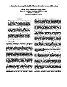
Figure 1.1: a) Map of Antwerp, Belgium. The red dot depicts the site of the only governmental air quality monitoring station (VMM) present in the urban area. b) The Aeroflex bike [25] is equipped with PM ,UFP monitors and GPS. c) Backpack equipped with air quality monitor devices (Fachhochschule Düsseldorf). d) Dustcart prototype robot developed in the framework of the DustBot project [48, 114]: the robot, while performing urban hygiene tasks, monitors pollution levels (PM10).

1.1. PROBLEM STATEMENT

3

A better assessment of the spatial and temporal variability of pollutants can be addressed either by densifying the pollution monitoring network using low cost gas sensor (e.g. metal oxide and electrochemical) nodes or by employing mobile platforms equipped with portable and reliable monitors. Low-cost gas sensors are commercially available for relevant pollutants. However, their utilization has several drawbacks because they are not specifically designed for use in ambient air (low concentrations, complex mixtures) and are hence not reliable. Reliable portable instruments exist for particulate matter monitoring, and with some training they can be used by non-specialist users. Their costs, however, are in the range of 6000-10000 Euro strongly limiting their wider utilization to dedicated applications (panels (b) and (c) in Figure 1.1). In a not so far future, autonomous mobile robots equipped with portable monitors, can replace human-carried mobile nodes and act as an autonomous wireless node in a monitoring sensor network. Using mobile robots for air quality monitoring has been addressed in the EU project DustBot [48,114], in which robot prototypes were developed to clean pedestrian areas and concurrently monitor the pollution levels (panel (d) in Figure 1.1). Sensor nodes carried by mobile robots offer a number of significant advantages compared to stationary sensors. With their-self localization capability, they are able to refine the selection of sampling locations and perform pollution monitoring with higher resolution: they can replace inactive sensor nodes or they could be sent in unmonitored areas. Moreover, they offer the option of source tracking (e.g. a leak of gas or to find explosives [75]), or be used as first aid and cleanup of hazardous or radioactive waste sites. Robots equipped with gas sensors could be integrated in already existing sensor networks (e.g. DustBot system [48,114] in panel (d) of Figure 1.1).

1.1

Problem Statement

In virtually all uncontrolled environments pollutants are advected by turbulent flow; thus they exhibit a chaotic structure that evolves in time and space [79]. The in situ sensors used in portable monitors (e.g. gas sensors) provide only information about a small spatial area around it (e.g. inlet or sensor surface). Therefore, gas concentrations (or pollution levels) gathered by a portable monitor, need to be processed to build representations of their spatial distribution: gas distribution models (GDM). Gas distribution models can provide comprehensive information about a large amount of gas concentration measurements, highlighting, for example, areas of unusual gas accumulation. They can also help in locating gas sources and in planning where future measurements should be carried out. The modelling of pollutants mostly fits into two categories: deterministic and statistical dispersion models. Deterministic dispersion models provide a link between theory and measurements and account for source dynamics and physico-chemical processes explicitly. As a drawback, those models require de-

4


tailed information, which is not always available. Statistical models do not depict the actual physical processes, but they treat the input data as random variables and derive a statistical description of the target distribution using a set of measurements to learn which is the expected pollutant concentration. Building statistical gas distribution models is the main task of this dissertation. It is a challenging task because of the chaotic nature of gas dispersal and because only point measurements of gas concentration are available. From a statistical point of view, the task of modelling a gas distribution can be described as finding a model that best explains the gas measurements and predicts new ones. At this point, we can state the general problem of interest in this dissertation. Problem: Given a set of geo-referenced measures of relevant pollutants, gathered by a mobile platform, the task to be solved is that of deriving a truthful representation of the observed gas distribution. In this thesis, we present statistically gas distribution modelling using autonomous mobile robots, but the algorithms proposed could be used by different types of mobile platforms (e.g. bicycle), given that they also provide georeferenced measurements.

1.2

Outline

The rest of this thesis is organized as follows: Chapter 2 starts by describing the random nature of turbulent gas distribution, then introduces the electronic nose (including a description of the gas sensors used in this thesis): a device that tries to mimic biological olfaction. This chapter further gives an overview of applications where the electronic nose is used for pollution monitoring in urban environments; it summarizes deterministic and statistical pollution modelling and it ends with an overview of gas sensing in the field of mobile robotics. Chapter 3 provides an in-depth description of the simulation software; hardware and experimental scenario developed and set up to test the proposed algorithms. It concludes with a short description of the system and prototype robots developed in the framework of the DustBot project, where I was chiefly responsible for the development of the air quality module embedded in the whole system. Chapter 4 introduces the Kernel DM+V algorithm used for statistical gas distribution modelling. Then it introduces a method to include wind measurements (Kernel DM+V/W) during the computation of the model, and it presents qualitative and quantitative results (obtained in one of the

1.3. CONTRIBUTIONS

5

simulation environment). Qualitative results are presented by discussing the structure of the modelled gas distributions; quantitative results are presented in terms of the algorithms ability in predicting unseen measurements. Chapter 5 presents the full evaluation and comparison of the Kernel DM+V and the Kernel DM+V/W algorithms in two simulation environments: a wind tunnel with a constant and laminar flow; a wind tunnel with turbulent wind field caused by an obstacle. For each environment, we consider different gas sensor trajectories (sweep, spiral and random) and two types of gas sensor response: an instantaneous and noise free response (ideal); a response that tries to mimic the real dynamics of the metal oxide gas sensors (real). The chapter also presents the predictive variance estimate maps, for the two investigated environments, and discusses how those maps may improve the quality of the statistical gas distribution modelling. Chapter 6 presents the evaluation and comparison of the Kernel DM+V and the Kernel DM+V/W algorithms in experiments performed with mobile platforms in different real world scenarios. We start considering a wind tunnel; then we present results in which a mobile robot monitors three different indoor environments and one in an outdoor area. The chapter also presents the predictive variance estimate maps, for all the investigated environments, and discusses how those maps may improve the quality of the statistical gas distribution modelling. The Chapter ends describing results obtained with the DustBot system in two outdoor setting: a courtyard in Pontedera (Italy) and a pedestrian square in Örebro (Sweden). We present and compare maps, computed with the Kernel DM+V algorithm, obtained with a reliable (and expensive) PM10 monitor (DustTrak 8520) and MOX gas sensor. Chapter 7 extends the statistical gas distribution modelling to three dimensions (Kernel 3D-DM+V) and introduces a method to include the local wind measurements in the computation of the 3D model (Kernel 3DDM+V/W). The algorithms are evaluated using a mobile platform in an indoor environment. Chapter 8 finally concludes this dissertation and summarizes its contributions and directions of future research.

1.3

Contributions

The major contributions of this thesis, as outlined in the previous section, can be summarized as follows: A simulation tool to evaluate gas distribution modelling algorithms (Chapter 3).

6


Ambient Monitoring Module in the framework of the DustBot project (Chapter 3). Evaluation of the Kernel DM+V algorithm in simulation and real world environments (Chapters 4–6). Kernel DM+V/W algorithm: a statistical approach to model gas distribution in chaotic environments taking into consideration the local wind information (Chapter 4). Evaluation of the Kernel DM+V/W algorithm in simulation and real world environments (Chapters 4–6). The computation of Predictive Variance map , together with the corresponding mean estimate maps, allows to obtain a more detailed picture of the gas distribution in the environment by highlighting area of high fluctuations (Chapters 4–7). Kernel 3D-DM+V algorithm: a statistical approach to model gas distribution in three dimensions (Chapter 7). Kernel 3D-DM+V/W algorithm: a statistical approach to model gas distribution in three dimensions taking into consideration the local wind information (Chapter 7). Evaluation of the extrapolation in three dimensions using the Kullback-Leiber divergence to compare 2D slices of the 3D gas distribution to a 2D model obtained with an independent gas sensor (Chapter 7). Kernel 3D-DM+V and Kernel 3D-DM+V/W algorithms evaluation in terms of their capability to estimate unseen measurements in real world experiments (Chapter 7).

1.4

Publications

Some of the work presented in this dissertation has been published in a number of journal and conference papers. The following list relates all publications, which directly contributed to the thesis, to the respective chapters. • Asadi S., Reggente M., Stachniss C., Plagemann C., and Lilienthal A.J. Statistical gas distribution modelling using kernel methods. In Evor L. Hines and Mark S. Leeson, editors, Intelligent Systems for Machine Olfaction: Tools and Methodologies, chapter 6, pages 153–179. IGI Global, 2011. (Contribution to Chapters 4–7 in this thesis). • Reggente M., Mondini A., Ferri G., Mazzolai B., Manzi A., Gabelletti M., Dario P., and Lilienthal A.J. The DustBot system: using mobile robots to

1.4. PUBLICATIONS

7

monitor pollution in pedestrian area. Chemical Engineering Transactions, 23:273–278, 2010. (Contribution to Chapters 3 and 6 in this thesis). • Reggente M. and Lilienthal A.J. The 3D-Kernel DM+V/W algorithm: Using wind information in three dimensional gas distribution modelling with a mobile robot. In Proceedings of IEEE Sensors, pages 999–1004, 2010. (Contribution to Chapter 7 in this thesis). • Reggente M. and Lilienthal A.J. Using local wind information for gas distribution mapping in outdoor environments with a mobile robot. In Proceedings of IEEE Sensors, pages 1715–1720, 2009. (Contribution to Chapters 4– 6 in this thesis). • Lilienthal A.J., Reggente M., Trincavelli M., Blanco J.L., and Gonzalez J. A statistical approach to gas distribution modelling with mobile robots–the Kernel DM+V algorithm. In Proceedings of the IEEE/RSJ International Conference on Intelligent Robots and Systems (IROS), pages 570–576, 2009. (Contribution to Chapters 4–6 in this thesis). • Reggente M. and Lilienthal A.J. Statistical evaluation of the Kernel DM+V/W algorithm for building gas distribution maps in uncontrolled environments. In Proceedings of Eurosensors XXIII conference, pages 481–484, 2009. Included in: Procedia Chemistry (ISSN: 1876-6196) Volume 1, Issue 1, 2009. (Contribution to Chapters 4–6 in this thesis). • Lilienthal A.J., Asadi S., and Reggente M. Estimating predictive variance for statistical gas distribution modelling. In AIP Conference Proceedings Volume 1137: Olfaction and Electronic Nose - Proceedings of the 13th International Symposium on Olfaction and Electronic Nose (ISOEN), pages 65–68, 2009. (Contribution to Chapters 4–6 in this thesis). • Reggente M. and Lilienthal A.J. Three-dimensional statistical gas distribution mapping in an uncontrolled indoor environment. In AIP Conference Proceedings Volume 1137: Olfaction and Electronic Nose - Proceedings of the 13th International Symposium on Olfaction and Electronic Nose (ISOEN), pages 109–112, 2009. (Contribution to Chapter 7 in this thesis). • Trincavelli M., Reggente M., Coradeschi S., Ishida H., Loutfi A., and Lilienthal A.J. Towards environmental monitoring with mobile robots. In Proceedings of the IEEE/RSJ International Conference on Intelligent Robots and Systems (IROS), pages 2210–2215, 2008. (Contribution to Chapters 4–6 in this thesis). Additional papers appeared as a result of this thesis but are not included in this dissertation:

8


• Reggente M., Peters J., Theunis J., Van Poppel M., Rademaker M., Kumar P., and De Baets B. Prediction of ultrafine particle number concentration in urban environments by means of Gaussian process regression based on measurements of oxides of nitrogen. Environmental Modelling & Software, in Press, 2014. • Peters J., Van den Bossche J., Reggente M., Van Poppel M., De Baets B., and Theunis J. Cyclist exposure to UFP and BC on urban routes in Antwerp, Belgium. Atmospheric Environment, 92(0):31–43, 2014. • Reggente M., Peters J., Theunis J., Van Poppel M., Rademaker M., Kumar P., and De Baets B. A comparison of monitoring strategies for prediction of utrafine particle number concentration in an urban air pollution sensor network. Science of The Total Environment (under review), 2014. • Elen B., Peters J., Van Poppel M., Bleux N., Theunis J., Reggente M., and Standaert A. The Aeroflex: a bicycle for mobile air quality measurements. Sensors, 13:221–240, 2013. • Mishra V.K., Kumar P., Van Poppel M., Bleux N., Frijns E., Reggente M., Berghmans P., Int Panis L., and Samson R. Wintertime spatio-temporal variation of ultrafine particles in a Belgian city. Science of the Total Environment, 431(0):307–313, 2012. • Di Rocco M., Reggente M., and Saffiotti A. Gas source localization in indoor environments using multiple inexpensive robots and stigmergy. In Proceedings of the IEEE/RSJ International Conference on Intelligent Robots and Systems (IROS), pages 5007–5014, 2011. • Ferri G., Mondini A., Manzi A., Mazzolai B., Laschi C., Mattoli V., Reggente M., Stoyanov T., Lilienthal A.J., Lettere M., and Dario P. DustCart, a mobile robot for urban environments: Experiments of pollution monitoring and mapping during autonomous navigation in urban scenarios. In Proceedings of ICRA Workshop on Networked and Mobile Robot Olfaction in Natural, Dynamic Environments, 2010.

Chapter 2

Background 2.1

Gas Dispersion in Natural Environments

In natural environments and virtually all uncontrolled environments, turbulent flow (caused by wind) is the dominant carrier for gaseous molecules. The dispersed gases exhibit a non-stationary (spatio-temporal) chaotic structure [79] that results in a concentration field of fluctuating irregular patches of high concentration. Panel (a) in Figure 2.1 shows the two mechanisms of gas dispersion obtained by solution of the equations of motion [44]. An area of uniform gas concentration (center), disperses and mixes in the environment due to the effect of molecular diffusion (left) or by advective turbulent flow and molecular diffusion (right). Molecular diffusion is the movement of molecules from a region of high concentration to one of lower concentration and it is described on a macroscopic scale by the Fick’s law: → − → − q = −D ∇c

(2.1)

where q is the rate of diffusion in three dimensions (per unit area and unit time), c is the mass concentration, and D is the molecular diffusion coefficient. Arrows indicate vector quantities; the minus sign indicates that the direction of transport is along the negative gradient. Molecular diffusion is a lengthy process: the diffusion velocity of ethanol at room temperature (25°C, 1atm and D=0.119 cm2 /s) corresponds to a mean velocity of 20.7cm/h [176]; in a coffee cup of 5cm height, the time for sugar to get uniformly mixed through the cup by molecular diffusion is about one month [185]. Molecular diffusion plays a crucial role only on small scales (it is important for e.g. bacteria) while in real world applications relevant to humans, wind is present and the dispersion and mixing are mainly due to advective turbulent flow. In every instant, a wide range of vortical flows (eddies) characterize the turbulent flow. Eddies act like diffusion if their size is smaller than the size of a patch of gas (panel (b) in Figure 2.1). Eddies comparable to the gas patch size 9

10

CHAPTER 2. BACKGROUND

(a)

(b)

(c)

(d)

(e)

(f)

Figure 2.1: a) The effect of turbulence compared to mere molecular diffusion, adapted from [44]. b) Diffusive eddy. c) Dispersive eddy. d) Advective eddy. e) Deformation of a chessboard patch in a dispersive eddy. f) Dispersion of a trace in a turbulent environment.

2.2. BIOLOGICAL OLFACTION

11

(panel (c) in Figure 2.1) cause distortion, stretching, and convolution of the patch. Those mechanisms accelerate the mixing process because they stir the gas patch irregularly over a larger volume. In panel (e) of Figure 2.1, dispersive eddies change and move the shape of a chess board. Eddies bigger than the patch of gas, instead, move the entire patch without contributing to its mixing (panel (d) in Figure 2.1). All those eddies contribute, for example, to the dispersion of a trace in a turbulent environment shown in panel (f) of Figure 2.1. The effect of the transport mechanisms in turbulent environments averaged over extended times can be modelled as [185]): ∂c ∂c ∂c ∂ ∂c ∂ ∂c ∂ ∂c ∂c +u +v +w = x + y + z (2.2) ∂t ∂x ∂y ∂z ∂x ∂x ∂y ∂y ∂z ∂z where, i are the eddy diffusivity coefficients that model the fluctuating parts of the turbulent flows.

2.2

Biological Olfaction

The olfactory system, which mediates the sense of smell, is probably the oldest sensory system in nature. The sense of smell is essential for the life of almost all creatures and important for e.g. finding food, avoiding predators or choosing a partner. Moreover, for many living organisms, the sense of smell is one of the most crucial mechanism for communication with the environment. In 1991 Richard Axel and Linda Buck clarified how the human olfactory system works, explaining the role of the receptors and how the brain interprets odors [24]. For their work, in 2004, Axel and Buck won the Nobel Prize in Physiology or Medicine. They discovered a gene family (which constitutes three percent of the entire human genes) that encodes around 400 different odorant receptors. Each of those correspond to an olfactory receptor cell. The olfactory mucous membrane is the region of the nasal cavity that contains the olfactory receptor cells. A larger area of olfactory mucous corresponds to higher olfactory sensitivity: humans have an area of olfactory mucous membrane of about 3–5cm2 ; in dogs, that have a highly developed sense of smell, the olfactory mucous membrane covers an area of 75–150cm2 . Each olfactory receptor cell reacts to odorous molecules with different intensity. Different odorant molecules activate different receptors (odorant pattern). The receptors send electrical stimulation to a microregion of the olfactory bulb (glomerulus). The brain interprets the activity in the different glomeruli (odorant patterns) as smell. This is the basis for the ability to identify and build memories of nearly 10000 different odors. Figure 2.2 shows the flow of the olfactory signal, from the activation of the receptors, due to the presence of an odorant, to the high regions of the brain.

12


Figure 2.2: Olfactory system (image adapted from [142]).

2.3. ARTIFICIAL OLFACTION – ELECTRONIC NOSE

2.3

13

Artificial Olfaction – Electronic Nose “An electronic nose is an instrument which comprises an array of electronic chemical sensors with partial specificity and an appropriate pattern recognition system capable of recognizing simple or complex odors” (Gardner and Bartlett).

Gardner and Bartlett in 1994 coined the definition of an electronic nose [182] as a device that attempts to mimic the discrimination of the mammalian olfactory system for smells. The research work that leads to this definition dates back to the 1920s when Zwaardemaker and Hogewind [77] made the first reported attempt to detect odors by measuring the electrical charge on a fine spray of water that contained odorant solution. Hartman in 1954 produced the first gas sensor [83]. The sensing element was a platinum wire of 0.8mm in diameter in contact with the surface of a porous rod saturated with a diluted electrolyte. By using various combinations of metal wires, electrolytes and potential biases, Hartman constructed an array of eight electrochemical cells which gave different patterns to different odorant samples. In the 1960s, studies of Seiyama et al. [177] demonstrated that semiconducting oxide surfaces (zinc oxide or tin oxide) change their properties according to different mixtures of air and gases interacting with the surface. In 1972 Taguchi patented the first tin dioxide based chemical gas sensor [141]. In the 1980s, Persaud and Dodd [97] and Ikegami and Kaneyasu [4] introduced the concept of an electronic-nose as an intelligent chemical sensor array for odor discrimination. The 1990s registered a remarkable increase of interest in this field: the first workshop on chemosensory information processing during a session of the North Atlantic Treaty Organization (NATO); an increase in published articles and industrial and commercial effort to improve electronic nose technologies. In this period, commercial electronic noses appear on the market (MOSES from ITT, and the Applied Sensor 3300). In the 2000s the electronic nose community received increasing interest also from different research communities, namely pattern recognition and mobile robots. Nowadays the basic architecture of an electronic nose is almost unchanged: in addition to the main components defined by Gardner and Bartlett [182] – a gas sensor array and a computational processing unit (CPU) – peripheral systems that sample and deliver the gas to the sensor array (Figure 2.3) are of interest in the gas sensor community. A well designed sampling system can considerably improve the performance of the electronic nose.

2.3.1

Gas Sensor Array

The sensor elements in an electronic nose have similar functions to the olfactory receptor cells in the biological olfactory system. Gas sensors measure the ambi-

14


Figure 2.3: Block diagram of an electronic nose. ent gas atmosphere based on the general principle that changes in the gaseous atmosphere alter the sensor properties in a characteristic way. Therefore, gas sensors are responsible for the transduction of odors into electronic signals. For realistic applications, gas sensors with a set of characteristics are desired: high sensitivity; high selectivity to a target gas; low cross-sensitivity to interferents (e.g. other gases, humidity or temperature); large dynamic range; perfect reversibility of the physicochemical sensing process; short sensor response and recovery time; long-term stability. However, as stated by Hierlemann and Gutierrez-Osuna in [3] “a sensor exhibiting all these properties is a largely unrealizable ideal”. Röck et al. [61] have stated that one of the main reasons why it has not been possible to accurately mimic the human nose is the high specificity of the human receptors in comparison to artificial gas sensors. The technical realization is always a trade off between high specificity and reversibility. High specificity demands irreversible interaction of the physicochemical sensing process. Despite progress over the last decades, it is chiefly the limitations of current gas sensor technology which ultimately prevent a substantial number of real-world electronic nose applications. Metal Oxide Gas Sensor - MOX Among the variety of different gas sensor transducer principles, metal oxide gas sensors (MOX) can be considered as one of the standard sensors in the field of electronic noses [61]. The reasons include that MOX gas sensors are commercially available, inexpensive to manufacture, have a high sensitivity and (depending to the application) can be used for a period of few years. Beside those advantages and the drawbacks common to other gas sensor types – selectivity, sensitivity and stability (3S problem) – they have additional disadvantages. MOX gas sensors require high working temperatures (200°C-500°C): the chemical reaction, which determines the gas sensor response, is extremely slow below 200°C. Consequently they need up to one hour to reach the working temperature before operation. Not micro-machined, gas sensors have high


15

power consumption (in the order of 800mW). With micro-machining technologies, the power consumption can be brought down to 75mW [147]. MOX gas sensors have also a slow recovery time after removing the target gas (15s to 70s). Panel (a) in Figure 2.4 shows the structure of a MOX gas sensor, comprising of a sensitive layer deposited over a substrate provided with electrodes for the measurement of the electrical characteristics of the device. MOX gas sensors comes with an in-built heater, separated from the sensing layer and the electrodes by an electrical insulating layer, which allows the sensor to operate at its working temperature. The change in conductance of the metal oxide, when a gas interacts with the surface of the sensing layer, is the principle of operation of metal oxide sensors. The change in conductance is correlated with the concentration of the reacting gas [95]. Panel (b) in Figure 2.4 shows a simplified representation of the physical and chemical processes that occur at an n–type gas sensor surface during 5 different phases: initialization; steady state in clean air; injection of a reducing gas; steady state in the presence of reducing gas; recovery after removing the reducing gas. Panel (c) in Figure 2.4 shows the ion density (top row) and conductance (bottom row) changes in each phase. During the initialization phase, the gas sensor is in clean air, and its surface heated up to reach the working temperature. As the surface increases its temperature, the oxygen present in the air starts to react with the sensing layer and starts to traps free carriers (electrons) at the surface in the form of ions: e+

1 O2 → O(s)− 2

(2.3)

where s refers to the sensor [76]. This results in an increase of ion density and a reduction of conductance, due to the lack of free electrons (phase 1 in panel (c) of Figure 2.4). When the surface reaches its working temperature, the sensor and the surrounding environment (clean air) are in a steady state, resulting in a constant ion density and low conductance (second phase). In phase three, a reducing gas (e.g. H2 S, CH4 , CO) starts to react with some pre-absorbed oxygen, or with some oxide present at the sensor surface, releasing electrons. Those reactions result in a decreased ion density and consequently an increased number of free electrons that increase the conductivity of the metal oxide layer: R(g) + O(s)− → RO(g) + e

(2.4)

where R(g) is the reducing gas, g refers to gas and s to sensor [76]. The change in the layer conductivity depends on the amount of free carriers, and, therefore, on the amount of reducing gas that reacts with the sensor surface. In the fourth phase, in which the amount of reducing gas is kept constant, which again results in a steady state between the sensor and the surrounding environment.

16


(a)

(b)

(c)

Figure 2.4: a)Structure of a metal oxide gas sensor. b) Simplified model of the physical and chemical processes occurring at the gas sensor (n–type) surface during five different phases. c) Changes of ion density (top row) and conductance (bottom row) in the five phases.


17

Gas sensor recovery (fifth phase) starts when the reducing gas is removed: the oxygen in the air starts again to trap electrons from the metal oxide resulting in a drop of conductance. The simplified model of Figure 2.4 refers to a family of sensors based on n– type sensing layers such as SnO2 ; ZnO; TiO2 ; WO3 . A second family of MOX gas sensors is based on p–type sensing layers (e.g. Cr2 O3 , Cr2−x Tiy O3+z or NiO). This family of sensors responds to oxidising gases like O2 , NO2 , and Cl2 that remove electrons. In this case, differently from n–type sensors, the reaction with the oxidising gas results in a drop of the conductance [139]. The simplified model presented above aims at giving an introduction of the basic mechanisms that drive changes in conductance of a MOX gas sensor. In [140] Barsan and Weimar, give a more accurate model which takes into consideration different sensing layer morphologies: compact thick and thin layers; porous layers (large and small grains). They also illustrate the role of electrode metal contacts (Schottky contact model) and the effect of different oxygen species on the surface depending on working temperature: molecular (O− 2) which dominates at temperature below 150°C and atomic ions (O− , O−− ) above 150°C.

2.3.2

Data Processing Unit

The second core component of the electronic nose is the data processing unit. It collects and integrates sensor signals – after conditioning – for further processing. In the first stage (pre-processing), the signals may require a reduction of noise, removing of anomalous data readings and/or data reduction (e.g. subsampling and averaging). Further, scaling of the signals coming from different sensors may help to cope with difficulties that derive from signals with different magnitudes. Baseline manipulation aims to compensate variations of the signals from their initial values in clean air, due to drift or changes in the environmental conditions (e.g. temperature and humidity). Three commonly used pre-processing methods are differential, relative and fractional [154, 182]. In the second stage, the data processing unit uses the pre-processed sensor signals together with techniques of pattern recognition to identify and quantify gases. Typically many applications handle the task of gas identification as a machine learning classification problem, determining the relationship that exists between a set of independent variables (the pre-processed signal from the different gas sensors) and a set of dependent variables (odour/gas classes) [154,182]. Quantification of the gases may be treated either as classification or regression problems. In the first case, gas concentration intervals are considered as a set of different classes. In regression, the gas concentration does not need to be discretized, and is instead treated as a real value variable. Many authors proposed different techniques to cope with the identification and quantification of gases. In [57] the authors provide a comprehensive

18


(a)

(b)

Figure 2.5: Response of a gas sensor array in closed (left) and open sampling systems (right). Adapted from [126]. overview of different multivariate methods and in [1] the authors reviewed statistical and biologically inspired classifiers. In Section 2.4.1, we discuss works that use pattern recognition techniques and gas sensors to monitor relevant pollutants (e.g. NOx, CO) in urban environments. In Section 2.5.2, we present works in which mobile robots, equipped with electronic nose, have the task to discriminate gases.

2.3.3

Delivery and Sampling Systems

The third component of an electronic nose (not included in the definition given by Gardner and Bartlett [182]) is a delivery and sampling system. This component determines in which way the gas is delivered to the gas sensor array. There are two types of sampling systems: closed and open. Closed sampling systems, usually refer to laboratory systems, where the gas sensor array is enclosed in a chamber, and environmental parameters, such as temperature and humidity are controlled. Closed sampling systems are predominantly used in electronic nose technologies, and a good design of the sampling system can substantially enhance the electronic nose performance. The established head sampling process requires the extraction of the gas sample (head space) and then its transfer to the chamber where the gas sensor array lies. In an open sampling system, the gas sensor array is directly exposed to the target gas. Open sampling systems are preferred in applications where a rapid response time is crucial, where the dimensions have to be small, in low-cost applications that employ simple devices or in systems with limited payload and/or limited power supply. The drawback is an increased difficulty in performing classification or quantification of gases. Panel (a) in Figure 2.5 shows a typical gas sensor array response in a closed sampling system. In this case, the time of exposure of the gas sensors to the gas

2.4. AIR POLLUTION MONITORING

19

is long enough to reach a steady state with the environment. The portion of the signal from the transient, steady state and recovery may be used for identification and quantification of gases. Panel (b) in Figure 2.5 shows an example of gas sensor signals collected by a mobile robot in an uncontrolled environment (open sampling system). In this case, the gas sensors do usually not have enough time to reach a steady state with the environment because the exposure to a constant gas concentration is too short. Therefore in an open sampling system only transients (rise and decay) can be used for identification and quantification of gases.

2.4

Air Pollution Monitoring

Air pollution monitoring is crucial to protect the public and the environment from harmful contaminants and pathogens in the air. The EU (Framework Directive 2008/50/EC) has imposed strict regulations on the concentration of various airborne environmental contaminants, which originate from different sources (e.g. vehicle emissions, heating systems and industrial processes [40, 53]). Pollutants of specific interest include nitrogen dioxide (NO2 ), carbon monoxide (CO), volatile organic compounds (VOC), ozone (O3 ), particulate matter (PM), especially ultrafine particles (UFP) and black carbon (BC) [35,67, 134]. Nitrogen dioxide (NO2 ) together with nitric oxide (NO) are known as nitrogen oxides (NOx). NOx emissions are associated with all types of hightemperature combustion, and the most influential sources in urban areas are the vehicles [56]. Direct NOx emissions from vehicles are mainly emitted as NO [149], which quickly reacts with ozone (O3 ) resulting in secondary NO2 formation [56]. The NO2 share of emitted NOx is increasing [113] due to the increased number of diesel vehicles, especially those that use exhaust aftertreatment systems (i.e. CRT - continuous regenerating trap) which use NO2 to regenerate the filter: soot particles are burned at 550◦ K using NO2 [153]. Carbon monoxide (CO) is a colourless, odourless and highly toxic gas that becomes lethal at high concentrations (∼800 ppm). In an urban environment typical CO concentrations are in the range of few ppm [106, 143]. Incomplete burning of fossil fuels is the primary source and in urban environments the main sources come from the transport sector, fuel-consuming industries and domestic fires. Volatile organic compounds (VOC) emissions result from incomplete combustion of fuels and from industrial applications that use solvents. Examples of its compounds are benzene and polyaromatic hydrocarbons. They are hazardous to humans and can cause blood diseases. Ground level or tropospheric ozone (O3 ) originates from the chemical reactions between NOx and VOC (ozone precursors) in the presence of sunlight. It is the leading source of photochemical smog, and it causes damage to plants,

20


eyes, lung and accelerates the degradation of rubbish materials. Ozone can also be transported by wind affecting rural areas. Particulates matter (PM) comprises dust, smoke, aerosols and any finely divided airborne solid material. Common sources are fires, motor vehicles, industries and natural emissions. The framework Directive 2008/50/EC regulates PM10 and PM2.5 (particles less than 10 and 2.5 µm in diameter, respectively) but not smaller. The particles smaller than 100 nm – ultrafine particles (UFP) [101] –, contribute most (around 80%) to the total particle number concentrations (PNCs) [102]. Road traffic can contribute up to 90% of total particle number concentrations [85, 160]. These particles can cause damage to pulmonary cells, may penetrate and deposit in the tissues, may also cause cardio-vascular damage [46] and could cause brain stroke when penetrating into the bloodstream and then being delivered to other organs [189]. From this list, it is clear that vehicles are the leading cause, directly and indirectly, of pollutants in an urban environment (an exhaustive analysis of traffic emissions, exposure, and related health effects is [80]). Therefore, the traffic related pollution is time and location dependent causing differences in pollutant concentrations over the day and between different micro-environments [30, 168]. The costs of the instrumentation, maintenance, calibration and infrastructures limit the number of traditional fixed monitoring stations (panel (a) in Figure 1.1) [96]. Therefore, current pollution monitoring networks are sparse, and they may not depict the differences between micro-environments properly. Rather high density networks that utilize traditional monitors are prohibitively expensive. On the other hand there is a need to improve monitoring capabilities: the ability to assess air quality at a higher spatial and temporal resolution can yield a considerable advance in understanding variability of pollutants in urban environments and their relationship to health effects, and thus the ability to determine the most appropriate and effective measures. A better assessment of the spatial and temporal variability of pollutants can be achieved by complementing the existing networks with affordable alternatives: using low cost gas sensors, modelling tools and mobile platforms. In this dissertation, we have mounted PM10 monitor and/or low cost gas sensors on mobile platforms (mobile robots) to gather geo-referenced measures of relevant pollutants, and we propose modelling tools to derive a truthful representation of the observed gas distribution.

2.4.1

Air Pollution Monitoring using Electronic Noses

Electronic noses can be used in a wide range of applications - in all cases where gases are involved - such as industrial, food quality, and pollution monitoring [7, 31, 61, 98, 175]. Low-cost gas sensors (e.g. MOX and electrochemical) are commercially available for relevant pollutants (NOx, CO, VOC and O3) [133]. However,


21

they are not specifically designed for use in ambient air where they are exposed to low concentrations and complex mixtures in an open sampling system. Specific strategies are required to compensate: short term drift due to daily changes in temperature and humidity; long term drift due to seasonal changes and ageing; cross-sensitivity to other gases (e.g. NO2 versus O3 ). In literature, there are only few works that deal with the drift counteraction under ambient conditions, in comparison to studies in laboratory conditions. Carotta et al. [131] [130] [132] presented studies of few days measurement campaigns (3 days up to one week) in an Italian city where they used thick-film gas sensors. They performed a field calibration using least square methodology for NOx and CO concentration estimation using as reference (target of the model) a governmental monitoring station. The sensors showed good sensitivity – comparable with the values that the reference monitor recorded – and short term drift counteraction. Because of the duration of their measurement campaign (few days), it is not possible to assess if their approach counteracts the long term drift. Tsujita et al. [186] used TGS 2106 (diesel exhaust sensors from Figaro Engineering [58]) in a gas sensor system to develop a low cost sensing node for a dense real-time environmental monitoring network. They proposed an autocalibration method that aims to achieve maintenance-free operation of the sensor network for NO2 monitoring. To perform auto-calibration, first they have statistically studied the NO2 concentration levels from four governmental monitors (around their sensor node) for a period of one year. They found that the NO2 concentration was almost uniform in the whole study area when the four station measured NO2 under 10ppb, and the wind speed was in the order of 4 to 5m/s. To correct the long term baseline drift, they proposed to adjust the gas sensor system output to the average of the NO2 concentration measured at the four governmental monitor stations when all stations simultaneously report concentrations less than 10ppb and the wind speed was higher than 4m/s. Their method to counteract the long term baseline drift is limited to the study area and to the local meteorological conditions. If the weather does not match particular meteorological condition the zero base line drift could not be calculated, and the auto calibration did not work. Kamionka et al. [111] presented a device (called “trisensors”) based on three sensitive tin dioxide (SnO2 ) thick films. Firstly, they calibrated the trisensor in the laboratory with synthetic air varying humidity and temperature combinations. Then they performed field calibration using reference analyzer measurements and a neural network (NN) to estimate NO2 and O3 levels. Their results were poor in terms of sensitivity and stability (calibration has to be performed every few days). They explained these results with the low quality of the solid state devices used to measure the pollutant levels. De Vito et al. [165] presented a low cost multi-sensor device based on seven solid-state sensors (5 gas sensors, one temperature and one humidity sensor) and a method to calibrate their device to estimate benzene levels. They cali-

22


brated their device directly in the field by placing their device next to a governmental monitor station. They used a statistical sensor fusion algorithm based on neural network (NN) regression, and in the training period they used the benzene data from the governmental station as reference (target of the model). They found that 10 days of training were sufficient to keep the mean relative error under a 2% threshold – with respect to the monitor station – and capable to limit the absolute prediction error (below 1µg/m3 ) for more than 6 months. In an extension of [165] to the estimation of CO and NO2 (with the same sensing device and for the same measurement campaign), De Vito et al. [166] found that 10 days of training, for their NN, were enough to achieve “satisfactory” results for 6 months CO and NO2 estimation.

2.4.2

Air Pollution Monitoring using Deterministic Dispersion Modelling

Deterministic dispersion models provide a link between theory and measurements [27] and account for source dynamics and physico-chemical dispersion processes (e.g transport mechanisms, chemical reactions) explicitly to calculate pollutant concentrations at various locations. Several dispersion models have been developed – for local and regional scales –, and they can be grouped (according to the modelling principle) in four categories: box models, Gaussian models, Lagrangian/Eulerian models and computational fluid dynamics (CFD) models. Box Models Box models (Figure 2.6) are based on the conservation of mass principle. The site of interest, that may range from a street canyon to the global atmosphere, is treated as a box that defines a volume of air. The air in the box receives pollution from sources while pollution is removed at the same time by a sink processes. The air pollutants inside the box are assumed homogeneously distributed; therefore, the model can predict only the volume-averaged concentration. The sources of the model are everything that introduces pollutants into the box: e.g. pollutants transported by wind; local emissions (cars); chemical formation. The sink processes, on the other hand, include all processes that remove or convert the pollutants: e.g. removal of pollutants by the wind (ventilation); deposition on the ground (rainfall); chemical conversion. The rate of change of concentration within the box is [172]: ∂h dc = LQ + uh(cb − c) + L(ca − c)max ,0 (2.5) Lh dt ∂t where c is the mean concentration within the box, cb the background concentration, ca the concentration above the boundary layer (h) and L the length


23

Figure 2.6: Schematic of the box model. of the box in the downwind direction. The first term on the right hand side of Equation 2.5 represents the emissions into the box, the second, replacement of polluted air by background air by advection, and the third, any reduction or increase in concentration due to entrainment of clean or polluted air aloft. In the case of zero background concentration and zero concentration aloft, the steady-state solution is: QL c= (2.6) uh Examples of software based on a box model are the street box module of AURORA (VITO, Belgium) [33], Canyon Plume Box (CPB, GEOMET) [159] and the Photochemical Box Model (PBM, US EPA) [167]. AURORA uses a steady state box model to calculate the concentrations of inert, reactive gases and particles within a street canyon with an output frequency of one hour, one day or one year. CPB uses an urban canyon box to calculate the average concentration of NO2 . PBM simulates photochemical smog at urban scale (typical horizontal dimensions are 10-50 Km) giving hourly concentrations of hydrocarbons and ozone. Gaussian Models Gaussian models assume that the plume in the down wind direction from a source follows a Gaussian distribution in the vertical and lateral directions under steady state conditions (panel (a) in Figure 2.7). 2 2 2 − y2 − (z−H) − (z+H) Q 2 2 2σz 2σz C= e 2σy e +e (2.7) 2πUσy σz where Q is the emission rate of the source, U is the mean wind velocity and H the effective stack height, that is the sum of physical stack height h and the plume rise dh – the plume normally rises above the stack because it is emitted at a temperature higher than ambient air and with a vertical velocity component. The concentration has its maximum at the center of the plume. The width

24


(a)

(b)

Figure 2.7: a) Visualization of a Gaussian air pollutant dispersion plume adapted from [45]. b) Puff model in steady-state (top) and not steady-state (bottom) conditions. of the plume, σy and σz , depend on the downwind distance (travel time) and the atmospheric stability class, that can be obtained using Pasquill-Gifford estimates [60, 62]. Since Gaussian plume models use steady state approximations they fit well only for relatively flat and homogeneous surfaces. They do not perform well under low wind condition or at sites close to the source (∼100m) or very far from the source (∼50km). Gaussian puff models, that approximate the plume as a series of puffs over time may overcome the steady state limitation allowing to model changes in wind speed and direction (panel (b) in Figure 2.7). Each puff is modelled using the Gaussian dispersion equation and the overall contribution, at the receptor site, is calculated by integration (in time) of the individual puffs and summation of the contribution of each puff. Examples of software that use a Gaussian dispersion model are CALINE4 (California Department of Transportation) [173] and HIWAY2 (US EPA) [188]. The traffic is treated as infinite line source split in elements that are located perpendicular to the wind direction. CALINE4 also considers the effects of thermal turbulence on vertical dispersion. CALPUFF [93] is an urban scale non-steady state puff model that describes the dispersion of gases and particles in domains, that may be complex or rough, from tens of metres to hundreds of kilometres at resolution time of one hour. CALLPUFF consists of three components: a meteorological modelling package; a Gaussian puff dispersion model with chemical removal, wet and dry deposition, complex terrain algorithms, plume fumigation, and other effects; post-processing programs for the output fields of meteorological data, concentrations and deposition fluxes.


25

Lagrangian and Eulerian Models In Lagrangian modeling, a packet of air/gas (puff) is followed along the downwind trajectory. The concentration at specific locations is given by the product of a source term and a probability density function as the puffs move from one point to another. The modelled pollutant concentrations can account changes due to mean fluid velocity, turbulence and molecular diffusion. In Eulerian modeling the area under investigation is divided into grid cells (vertical and horizontal). Pollutants enter and leave each cell (similar to the box model), and the model computes the pollutant concentrations at all locations as a function of time. Software packages that use Lagrangian or Eulerian models are GRAL (Graz University of Technology, Austria) [43], SPRAY (Arianet and Aria Technologies, Italy-France) [37] and FARM (Arianet, Italy) [32]. GRAL is a coupled Eulerain (mesoscale) and Lagrangian (microscale) model designed to model the dispersion of inert compounds within inhomogeneous wind fields. The model offers time resolutions from 10 minutes up to one hour, and a minimum spatial resolution of one meter for line and point sources within smooth and complex terrain. SPRAY (Lagrangian) computes concentrations and deposition of non-reactive emissions over complex terrain. The model offers time resolution from one minute, and a minimum spatial resolution of one meter. The FARM model (Eulerian) calculates concentration and deposition of reactive pollutants, particles and photochemistry gases between 500m up to 50km. Computational Fluid Dynamic Models – CFD CFD models provide complex analysis of fluid flow based on conservation of mass and momentum by resolving the Navier-Stokes equations using finite difference and finite volume methods in three dimensions. Turbulence is modeled using different formulations, e.g., the Reynolds-averaged Navier-Stokes approach (k– model, RNG k– model, Realizable k– model), and the LargeEddy Simulation (LES) approach. These models are useful for studies requiring high time–space resolution (usually in street canyons or near road studies). Drawbacks are that they are complex, resource demanding and a thorough validation is not straightforward. ENVI-met (University of Mainz, Germany) [108] is a micro-climate and local air quality model with time resolution of few seconds. Typical domains are: single street canyons; few hundred square meter areas. MERCURE (Aria, France) [42] has been used to model real time pollutants from vehicles in urban environments.

2.4.3

Air Pollution Monitoring using Statistical Modelling

Statistical models are techniques based essentially on statistical data analysis of measured ambient concentrations. These models do not model the actual

26


physical processes, but they treat the input data as random variables and derive a statistical description of the target distribution from a set of measurements. Statistical models can be used in order to infer expected concentrations under the assumption that the random process, which generated the pollutant distribution, has not changed. Statistical approaches offer complementary strengths compared to the deterministic dispersion models. These models do not rely on the validity of the underlying physical model, can provide a higher resolution and are computationally less expensive. Moreover, they are less demanding in terms of the required knowledge about the state of the environment. Interpolation Models Interpolation models rely on stochastic geostatistical techniques. These models use measurements of pollutant from a set of monitoring stations to estimate the pollutant concentration at sites other than the location of monitoring stations. Wong et al. [49] identified 4 interpolation models for air pollution exposure assessment: spatial averaging, nearest monitor (a nearest neighbour technique), inverse distance weighting, and kriging (also known as Gaussian Process regression). Among those methods, kriging offer the advantage of estimating both predicted values and their standard errors (kriging variance) at unsampled locations. The kriging variance quantifies the degree of uncertainty of the mean predictions, illustrating where the interpolation is not reliable. Ordinary kriging assumes no global trend in the data and the pollution is dependent on the distance between the measurement locations assuming a spatially homogenous variation. An extension is universal kriging that incorporates a drift function to account for global trends of the pollutant [90, 110]. Kriging has been used, for example, to estimate sulfur dioxide in [121], ozone [90] and particulates [39]. The quality of geostatistical interpolation depends on the availability of monitoring data and requires a reasonably dense network of sampling sites [110]. Land Use Regression – LUR Land use regression (LUR) is based on the principle that at any location the pollutant concentration depends on the characteristic of the surrounding site, in particular those features that are more informative about emissions and dispersions. Least-squares regression modelling is used to model the relationship between the measured concentrations and variables that describe the land characteristic of the sampling site and areas of influence around it (called buffers). The resulting regression model is then used to predict concentrations at different locations on the basis of these buffers. Briggs et al. [47] used a LUR model to predict the mean NO2 at 8 sites, using road traffic, land-use type and altitude. Their model explained up the 87% of the variance for the annual mean. Brauer et al. [107] predicted PM2.5 in multiple European cities and they showed that a multiple regression technique produces statistically reliable re-


27

sults. Jerret et al. [110] have shown that LUR models better capture small-scale and intra-urban variability than kriging and, that LUR models have relatively lower computational cost compared to dispersion models. The main limitation of this method arises from its area-specificity, for example, when moving to study areas with much different land-use (e.g. commercial to industrial) and topography. Air Quality Forecast with Statistical Signal Analysis Statistical techniques (e.g. regression, time series analysis, artificial neural networks) have been used, for alerting purpose, to forecast air pollution trends a few hours in advance. Among the forecast models, the accuracy of neural network (NN) prediction is often higher other forecast models [150]. The main reason is because NN can deal with non-linearities in the noisy data and may work with a large number of input variables [137]. In [86] the authors trained a multilayer perceptron to predict surface ozone concentrations in an industrialised area from the maximum daily temperature, CO2 , NO, NO2 concentrations and wind information. Their model was found to outperform linear regression and time-series analysis. Gardner and Dorling [138] trained a multilayer perceptron on hourly meteorological data (input) to predict hourly NOx and NO2 concentrations for the Central London area. Recently, non linear regression has been used to predict ultrafine particles (UFP) number concentrations. Mølgaard et al. [27] used Bayesian supervised regression on meteorological and traffic data to predict UFP number concentrations at an urban background monitoring station in Helsinki up to two days ahead. Clifford et al. [164] used data from the same monitoring station (2004–2006) to model the UFP number concentrations using a generalised additive model and meteorological data, time, solar radiation and rainfall as input. Reggente et al. [120] estimated the UFP number concentrations by means of Gaussian process regression at three urban site situated within a 1km2 area in a Belgian city, Antwerp. They inferred UFP concentrations based on the concentrations of NO, NO2 , CO and O3 at half hour and five minutes resolution. Because UFP number concentrations follow from a dynamic process, they used a non-stationary kernel based on the addition of a linear and a rational quadratic kernel. Their method provides accurate predictions when using NO and NO2 as covariates and less accurate predictions when using CO and O3 . Moreover, they found that training period of at least seven days is suitable to let the models learn the UFP number concentration dynamics in different typologies of traffic. In [119] Reggente et al., using the same measurement campaign, extended the previous work proposing three prediction strategies – local, remote and mixed – to estimate UFP number concentrations in an urban air pollution sensor network. They found that: (i) UFP number concentrations can be predicted with good accuracy based on NO/NO2 measurements at the same location; (ii) it is possible to predict UFP number concentrations at one location based on measure-

28


ments of NO/NO2 and/or UFP at two remote locations; (iii) the predictions can be improved adding, at the remote covariates, local measurements of gaseous components to take into account local variability.

2.5

Mobile Robots with Electronic Noses

Mobile sensors can be used to improve the spatio-temporal resolution of pollution monitoring networks [104, 155]. The use of mobile devices can generate additional information in locations where stationary measurements are lacking. In this section, we discuss works in which, mobile-robots carry portable devices to sense gases in the environment and can be employed in the pollution monitoring task. In particular, we focus on gas distribution modelling (GDM, Section 2.5.1) and the Kernel DM algorithm [17] that is at the base of the algorithms presented in this dissertation. Autonomous mobile robots equipped with an electronic nose systems (mobile nose or m-nose) can serve as autonomous wireless nodes in a monitoring sensor network. Sensor nodes carried by mobile robots offer a number of important advantages compared to stationary sensors. With their autonomy and self localization capability, they are able to refine the selection of sampling locations and perform pollution monitoring with higher resolution: mobile sensor nodes, can replace inactive nodes or they could be sent to unmonitored and potentially hazardous areas. Moreover, they offer the option of source tracking (e.g. finding a leak of gas or explosives [75]), or be used as first aid and cleanup at hazardous or radioactive waste sites. Robots equipped with portable monitors and/or gas sensors could also be integrated in already existing sensor networks: for example, in the framework of the EU project DustBot [48, 114], robot prototypes cleaned pedestrian areas and concurrently monitored pollution levels. Research on using chemical sensors in robotic systems started in the early 1990s essentially focusing on two tasks: first, following odor trails marked on the ground as ants follow a pheromone trail [156] (trail guidance, Section 2.5.4). Second, tracking odor trails in fluid media (air or water) to locate a chemical source [71] (gas source localization, Section 2.5.3). Complementary to these approaches, the production of chemical distribution maps (gas distribution modelling – GDM described in Section 2.5.1) aims to model the actual distribution of a gas in an area of interest and, therefore, may also provide the means to localize a pollutant source [78]. Recently, a new area of interest is emerging: Trincavelli and Loutfi, in a series of works, have proposed algorithms for discrimination of gases in uncontrolled environments [6,122,124–127] (Gas Discrimination with mobile robots Section 2.5.2). This dissertation focuses on gas distribution modelling (GDM); therefore, we will describe in detail only works related with this topic. In the literature, almost the entirety of the publications consider a 2D environment, and the works that consider a three dimensional environment are still rare. In Chapter 7, we

2.5. MOBILE ROBOTS WITH ELECTRONIC NOSES

29

will present an algorithm to model the gas distribution in three dimensions, and in the same chapter we will describe works that consider the three dimensional environment.

2.5.1

Gas Distribution Modelling – GDM

Modelling the distribution of gas in an environment aims at deriving an accurate representation of the observed gas distribution from a set of spatially and temporally distributed measurements of relevant variables, foremost gas concentration, but also wind, pressure, and temperature [12]. Building gas distribution models is a difficult task mainly because in realistic scenarios turbulent advection disperses the gas (Section 2.1), and because the predominantly used in situ gas sensors provide information only about a small spatial region, the sensor surface that reacts with the environment. Therefore, instantaneous measurements of gas concentration over a large area would require a dense grid of sensors which is usually not a viable solution due to the high cost and lack of flexibility. Gas distribution modelling (GDM) methods can be categorized as modelbased and model-free. Model-based approaches infer the parameters of an analytical gas distribution model from the measurements. In principle, Computational Fluid Dynamics (CFD) models can be applied to solve the governing set of equations numerically. Current CFD methods are computationally expensive, and they are not suitable for realistic scenarios. Many other model-based approaches were developed for atmospheric dispersion (Section 2.4.2). Such models typically cannot efficiently integrate sensor information on the fly and do not provide a sufficient level of detail. Simpler analytical models, as in [78], often rely on rather unrealistic assumptions and are only applicable for situations in which the model assumptions hold. Approaches based on an analytical model also depend on well-calibrated gas sensors, an established understanding of the sensor-environment interaction and often on knowledge about the gas source intensity and location. Model-free approaches do not make strong assumptions about a particular functional form of the gas distribution. They typically treat gas sensor measurements as random variables and derive a statistical model of the observed gas dispersion from the measurements. An intuitive solution to build a model of the time-averaged gas distribution is the work of Hishida et al. [78]. They used measurements acquired by a network of fixed sensors, and they averaged the sensor readings over a prolonged period (5–8 minutes). To visualize the map, they discretised the averaged values to a grid that represents the topology of the sensor network. This solution offers the convenience of reduced time consumption to create a map, but it requires considerable effort in sensors calibration and maintenance. Figure 2.8 shows a gas distribution map created in this way: the black dots indicate the location of 33 gas sensors in a clean room; the white circle represents the gas source;

30


Figure 2.8: Time-averaged gas distribution map computed by 33 grid points sensor readings in a clean room environment (adapted from [78]). the arrow shows the direction of the wind stream. The gray scale represents the gas concentration in the room. Brighter areas denote lower concentrations of the target chemical and the darker areas denote higher concentrations (corresponding to low resistance of the sensor). It can be seen that the plume extends well away from the gas source following the wind direction. Purnamadjaja and Russell [9] used a similar method: instead of average values they mapped peak values observed in a period of 20 seconds (arena area about 1×2.5m2 ). Under the assumption of stationary gas distribution, the utilization of only one gas sensor mounted on a mobile platform that consecutively collects gas sensor values, is equivalent to simultaneous distributed measurements. While a network of sensors has advantages in terms of coverage and sampling time, using a mobile sensor avoids calibration issues and allows for adaptive sampling of the environment. Pyk et al. [148] produced a gas distribution map by using a single sensor array (panel (a) in Figure 2.9). They collected consecutive measurements in 63 equally distributed locations (yellow dots), in a wind tunnel (area of 4×3m2 ) with an airflow of 0.67m/s. They built the gas distribution map by averaging the measurements over 2 minutes, and to make predictions at locations different from the measurement points they used bi-cubic interpolation. The gas distribution map in panel (a) of Figure 2.9 presents a plume-like structure and the higher values (in red) are found in the proximity of the gas source location – at grid point (0m, 1.5m). As a further step, Pyk et al. [148] mounted a sensor array on a mobile robot, driving it with a speed of 0.1m/s with a zig-zag trajectory, in the same wind tunnel. Since the measurement locations are not equally distributed, as in the previous case, they interpolated the readings using triangle based cubic filtering. Panels (b) and (c) in Figure 2.9 display the maps computed using one sweeping-run of the wind tunnel and by the average of three runs respectively. The dashed line indicates the trajectory of the robot and the gas source location is the same as in panel (a). The gas distribution maps obtained in experiments with the mobile robot present a jagged distribution (panels (b) and (c)), re-

31


(a)

(b)

(c)

Figure 2.9: Gas distribution map in a wind tunnel adapted from Pyk et al. [148]. a) Map obtained from sequential measurements with a single sensor array. b) Map created from the response of a gas sensor array mounted on a mobile robot at a speed of 0.1m/s. The dashed white line represents the robot’s path. c) Map computed by averaging the measurements over three runs of the robot.

(a)

(b)

(c)

(d)

Figure 2.10: Gaussian process mixture approach. a) Means of the two mixture components (background and high concentration). b) Gating function. c) Gas distribution computed with the GPM model and d) with a single GP model. In all plots, blue represents low, yellow reflects medium, and red refers to high values. Adapted from [34]. vealing a limitation of the spatial interpolation of the gas sensor readings: the fluctuations appear in the map even if they were close to each other. Hence the map obtained by averaging over three runs (panel (c)) presents an even more irregular distribution than the map created from a single run (panel (b)). Marques et. al [99] used 5 robots to collect gas measurements in a ventilated room. They fused the gas measurements and the wind speed using a non turbulent advection-diffusion model. They divided the experimental arena into grid-cells and represented the gas concentration in each cell by one state variable of a Kalman filter. Blanco et al. [92] used a Kalman filter for sequential Bayesian estimation on a 2-d grid assuming a stationary distribution. Stachniss et al. [34] proposed to consider gas distribution modelling as a regression problem. They proposed a sparse Gaussian process mixture (GPM) model: one component of the GP mixture represents the relatively smooth background signal and another component models patches of high concentrations.

32


(a)

(b)

(c)

Figure 2.11: a) Experimental arena used in [22]. b) Visualisation of the number of odour hits (i.e. how often the sensor response exceeded a predefined threshold) recorded by the six robots. c) Two-dimensional histogram which is obtained by accumulating the odour hits received by all the robots. A gating function decides to which mixture a data point belongs. Stachniss et al. used the expectation maximization (EM) algorithm to learn the gating function and the hyper-parameters of the mixture models. They tested their approach using the datasets described in Section 3.2.3. Panels (a) and (b) in Figure 2.10 show the mean predictions of the two mixture components (background and high concentration) and the gating function after EM convergence, respectively. Panels (c) and (d) of Figure 2.10 show the mean prediction of the final mixture model and a single Gaussian process (GP) model respectively. As can be seen, the mixture model presents a sharper boundary around the gas concentration peak (which is in the proximity of the gas source location) than the single GP model. These maps refer to the three rooms described in Chapter 3. Hayes et al. [22] proposed to build a two-dimensional histogram representation of the gas distribution. They used a group of six robots that simultaneously covered the area of interest – an arena of 6.7×6.7m2 (panel (a) in Figure 2.11) – performing a random walk behaviour. The robots were equipped with conducting polymer sensors (fast response time: ∼100ms) to measure water vapour created by a hot water pan behind a fan (the airflow had an average speed of approximately 1m/s). The arena was divided into two-dimensional bins in which they recorded the number of odor hits received by all the robots. An odor hit was counted whenever the response level of the gas sensors exceeded a defined threshold. Panel (b) in Figure 2.11 shows an example of the odor hits collected by the six robots and panel (c) in Figure 2.11 shows the estimated plume using all the odor hits collected by the robots. This approach has some limitations: first, due to the binary nature of the input, the map strongly depends on the chosen threshold and bin size, with the risk that useful information may be discarded. Second, the robots have to cover entirely all the area of interest to produce a reliable map. Third, the approach depends on the bin size and there is not spatial interpolation of the odor measurements, therefore, the coverage


33

time increases quadratically if the size of the investigated area increases assuming a fixed number of robots. Kernel DM The kernel distribution mapping (Kernel DM) algorithm, presented by Lilienthal and Duckett [17], has inspired the algorithms presented in this dissertation. The Kernel DM is inspired by non-parametric estimation of density functions using a Parzen window [52] (see Appendix A) and can be regarded as a refinement of the histogram-based approach [22] (presented above) with the difference that it does not depend on the assumption of an even coverage of the environment because it performs spatial extrapolation of the (gas) sensor measurement. At the core of the algorithm is the Nadaraya-Watson estimator [54], and the spatial extrapolation of the (gas) sensor measurement is the key idea of the Kernel DM algorithm. The sensor measurements provide information about a small area around its surface, which interacts with the environment, and the Kernel DM algorithm extrapolates this information using a Gaussian weighting function for locations at a certain distance from the sensor surface. Kernel DM represents a gas distribution in the form of a grid map. The area of interest is divided into grid cells and the algorithm computes an estimate of the distribution mean for each cell by using a symmetric Gaussian kernel N. The kernel represents a weighting function that indicates the likelihood that the measurement represents the average concentration at a given distance from the point of measurement. Considering a set of gas sensor measurements ri obtained at location xi the first step of the Kernel DM is to calculate the displacement of the measurement location xi from the centre of each grid cell k: (k)

δi

= |x(k) − xi |

(2.8)

using this distance, the value of the weight function (kernel) for a given measurement is computed for each cell by: (k)

(k)

ωi (σ) = N(δi , σ).

(2.9)

Where, σ – kernel width – governs the amount of extrapolation. The choice of σ is a trade-off between extrapolation on single measurements and the level of detail at which the gas distribution can be modelled. The parameter σ corresponds to the model complexity, a high value results in smooth models and small values allow for more complex models. The following step is the computation of two temporary maps Ω(k) and (k) R that represent integrated weights (corresponding to the density of measurements) and integrated weighted readings respectively: Ω

(k)

=

n X i=1

(k)

ωi (σ),

(2.10)

34


Figure 2.12: Evolution of a gas distribution map computed with the Kernel DM algorithm (σ = 0.15m). The gas measurements are collected with a gassensitive mobile robot that followed a predefined path (orange line). Concentration values are indicated by shadings of grey (dark shadings correspond to low concentrations, and light shadings to high concentration), while the values higher than 90% of the maximum concentration value are shown with red shadings. The black circle represents the location of the gas source, the blue and green dots represent the maximum and the median respectively (adapted from [17]).

R(k) =

n X

(k)

ωi (σ)ri .

(2.11)

i=1

Finally, the estimate of the distribution mean for each cell is computed as r(k) = R(k) /Ω(k) : Ω(k) > Ωmin

(2.12)

where, the integrated weights Ω(k) are used for normalisation of the weighted readings R(k) , thus perfectly even coverage is not necessary. The threshold Ωmin makes sure that estimates are based on a sufficient amount of measurements collected in the vicinity of their location. Figure 2.12 shows the evolution of the grid maps, computed with the Kernel DM algorithm, during one experiment. Concentration values are indicated by shadings of grey (dark shadings correspond to low concentrations, and light shadings to high concentration) while the values higher than 90% of the maximum concentration value are shown with different shadings. Kernel DM extensions Recently, several works presented extensions of the Kernel DM algorithm. Lilienthal et al. [10] took into account for the uncertainty about the sensor position: they integrated gas distribution mapping into a SLAM framework. In [12] Lilienthal et al., beside the estimate of the mean, modelled the spatial


35

Figure 2.13: Gas distribution maps adapted from [179]: classification map (left); mean map (middle); variance map (right). The black dashed lines denote the robot’s trajectory. The green and red circle denote the locations of the ethanol and 2-propanol source. structure of the distribution variance (Kernel DM+V algorithm, see Chapter 4), providing relevant information about the gas distribution by highlighting areas of high fluctuation. Asadi et al. [163] presented an approach to overcome the assumption that the gas distribution is generated by a time-invariant random process. They combined the spatial extrapolation of the Kernel DM+V algorithm with temporal extrapolation weighted by a time-dependent term defined with a time-scale factor (TD Kernel DM+V). In other words, they assumed that more recent sensor readings carry more valuable information in order to predict future measurements. In [6] Loutfi et al. addressed the task of integrating the classification of gases with gas distribution mapping. They performed experiments with a mobile robot in large and unmodified indoor and outdoor environments. An ethanol gas source was placed in the indoor section of their experimental area, and an acetone source in the outdoor section. Gas classification was performed using the transient information of the gas sensor measurements and a set of Debauchies discrete wavelet transforms as features and support vector machine (SVM) classifier to distinguish between ethanol and acetone. Hernandez Bennetts et al. [179] presented an algorithm that creates gas concentration maps in a situation where multiple heterogeneous gas sources are present (MC Kernel DM+V) fusing spatial extrapolation, classification and quantification of gases. They used an array of MOX sensors and a pattern recognition algorithm (multi variate relevance vector machine) to identify the compound, and a photo ionization detector (PID) for the quantification. They build a map for each compound (ethanol, 2-propanol and fresh air) using the Kernel DM+V algorithm (Figure 2.13). They tested their approach in experiments where a mobile robot carried the gas sensors and the PID in a room with two gas sources (ethanol and 2-propanol). Figure 2.13 shows an example of the obtained classification map (left), mean map (middle) and variance map (right).

36


Local airflow – due to the strong influence of advective transport – is a fundamental parameter for gas dispersal. In Chapter 4, we will describe how to integrate the local wind information in the computation of the gas distribution map, by adjusting the shape of the kernel using the measured wind direction (Kernel DM+V/W algorithm). Neumann et al. [151] used the Kernel DM+V/W algorithm (proposed in this dissertation) to build areal gas distribution maps using a flying drone in experiments conducted in a geochemically active region in Tuscany (Italy). In Chapter 7, we will present a further extension of the Kernel DM algorithm: how to build three-dimensional gas distribution maps (Kernel 3D-DM+V/W algorithm) including local wind information when available.

2.5.2

Gas Discrimination with mobile robots

Gas Discrimination with mobile robots is a new field in the robotic olfaction domain, and it has gained increasing interest in recent years. Almost the totality of the algorithms described in this thesis make the assumption of the presence of only one gas source, not considering the problem of gas discrimination. Many research groups have proposed algorithms for gas discrimination under laboratory condition (closed sampling systems), either using gas sensor steady state response or transient information [3]. The situation differs in robotic applications, where gas sensor arrays are exposed directly to the environment (open sampling systems), without the utilization of a gas chamber. In an open system, due to the chaotic nature of the uncontrolled environment, the discrimination of gases is more challenging than in a closed system because the discrimination of gases has to be performed in the early stage of the transient response of the gas sensor. Trincavelli and Loutfi implemented most of the work in this field. Trincavelli et al. [124,126], designed and implemented discrimination algorithms for open sampling systems. They were able to discriminate between three gas sources using data from an e-nose composed of five tin oxide sensors mounted on a mobile robotic platform. They performed experiments in an enclosed indoor and outdoor environment. In the outdoor environment, they were able to discriminate the gases using the information gathered in the indoor experiments as training set. They also analysed the classification performance depending on the distance of the gas sensor array from the gas source and did not find a strong correlation in the close range (classification errors occurred both close to the source and several meters away from the source). In [127], they have extended the algorithm for navigation purposes. The classification algorithm ran online and gave input to the path planner to optimize the robot’s path with respect to the gas discrimination task. In [125], they have proposed to use an ensemble of classifier to improve the discrimination, and in [122] they proposed a feature selection method to improve the gas discrimination in an open system.

37


Table 2.1: Gas source localization categories proposed in [174] Methods

Gradient ascent

Bio-inspired

Probabilistic inference Map-based Other approaches

2.5.3

Techniques One gas sensor, biased random walk Two sensors on a single robot, the sensor difference can be used for robot navigation Particle swarm optimization (PSO) Upwind surge Spiraling Casting Infotaxis Odor concentration maps Combination of vision, olfaction and airflow maps Avoiding high concentration region

References [2, 5, 100, 161] [13, 15, 18, 20, 21, 41, 72]

[100, 183] [91, 148] [22, 23, 66] [50, 72, 89, 161, 184] [129] [12, 16, 34, 88] [68] [15, 18]

Gas Source Localization

Gas source localization, with mobile robots, aims to find the location of a gas source that releases some chemical substance in the environment. Since the beginning of the mobile robot olfaction research, gas source localization is the most frequently studied problem. Several research groups proposed different approaches: Kowadlo et al. [69] reviewed and classified more than 25 algorithms in a Venn diagram; Lochmatter in his Ph.D. thesis [174] has classified the gas source localization algorithms in ten categories, which belong to five main categories, depending on the technologies used. Table 2.1 summarizes the classification that Lochmatter proposed. In this thesis, we do not propose algorithms for source localization, but the gas distribution map algorithms that we proposed in this thesis (Chapters 4– 7) compute the variance estimate map, that was experimentally found to give information about the gas source location.

2.5.4

Trail Guidance

The aim of trail guidance in mobile olfaction is to follow a chemical trace on the ground. A well known example from the biological life is the ants that follow and release pheromone trail to a source of food. Mobile robots used for trail guidance applications, usually mount a gas sensor at a close distance to the ground (∼1cm), therefore, the effect of the turbulent environment is small. Many research groups have proposed algorithms and devices for different ap-

38


plications. An in-depth description algorithms and devices is out of the scope of this thesis and the interested reader can find a good review in [11].

Chapter 3

Experimental Setup The algorithms that we propose in this dissertation could be used in different experimental situations and with different sensing platforms. Thanks to the collaboration with other research institutes we had the opportunity to realize the research ideas in different representative experimental setups and environments. This chapter introduces the experimental scenarios and sensing setups used. The first part describes the simulation environment used to develop and test the gas distribution modelling algorithms. The second part introduces the real world experimental scenarios: starting from a wind tunnel with a quasi-laminar flow of 1m/s up to a turbulent outdoor environment.

3.1

Simulation Setup

In the following sections, we describe the software (4 modules) employed to assess the gas distribution modelling algorithms in simulation environments: advection model; gas dispersion model; gas sensor model; robot path model. As advection model (Section 3.1.2)1 , firstly, we have used a laminar and uniform wind flow model of 1m/s without any obstacle, and then we have used a turbulent flow model with the presence of one obstacle. To model the dispersion of the gas, we used a model that closely resembles the filamentbased model, proposed by Farrell et al. [87] (Section 3.1.3). For the gas sensor response model (Section 3.1.5), firstly we have used an ideal response model – instantaneous and noise-free response. As a further step, we have employed a model of the dynamics of the MOX gas sensors, adding noise and transients (rise and decay) in its response. For the robot’s path model, (Section 3.1.4) we have considered three different strategies: sweep, spiral and random paths. 1 The author would like to thank Sepideh Pashami for her help in the phase of developing the simulation tools.

39

40

CHAPTER 3. EXPERIMENTAL SETUP

Figure 3.1: Sketch of the simulated experimental arena: wind tunnel. Arrows indicate the wind flow inlet; the gas source and the gas source outlet are shown in the left part. The gas plume (visualized by a cloud of gray points) is obtained using the gas filament distribution model proposed by J. Farrell [87] (Section 3.1.3).

3.1.1

Wind Tunnel Experimental Arena

The experimental arena considered is a rectangular area of 16m length and 4m width (Figure 3.1), which corresponds roughly to the dimensions of the wind tunnel used in the real world experiments described in Section 3.2.1. In Figure 3.1 the gray circle (at 1m from the left end of the arena), represents a circular gas source of 0.12m radius. The arena is discretised into a grid of around 6000 lattice points with a spacing of 0.1m in x and y direction. Each lattice point k stores its coordinates (xk ,yk ); the gas concentration value Ck,t at a certain time t (given by Equation 3.8) and the wind field value (uk,t , computed with the advection model described in Section 3.1.2).

3.1.2

Advection Model

For turbulent flow models, we have used the OpenFOAM program to model the airflow that is responsible for advection [145]. OpenFOAM is a free CFD software package produced by a commercial company (OpenCFD Ltd), licensed under the GNU General Public License (GPL). OpenFOAM is an open source software, and its core technology is a collection of C++ modules. Moreover its solvers, utilities and libraries are extensible. Laminar Flow Model The first advection model that we have used in the simulation experiments is a constant wind field of 1m/s without any turbulence. This model is extremely easy to implement, and it does not require the utilization of any software. In

41

3.1. SIMULATION SETUP

the coordinate system indicated in Figure 3.1, the wind vector at lattice point k, uk,t , can be written as:   1 uk,t = 0 (3.1) 0 This model roughly corresponds to the quasi-constant and laminar flow that we have used in the real wind tunnel (Section 3.2.1). Turbulent Flow In many real-world applications, obstacles and generally turbulence affect gas dispersion (Section 2.1). To assess if the gas distribution modelling algorithms presented in this dissertation are able to deal with turbulent gas dispersion we have employed an additional advection model that considers turbulence and obstacles. The scenario is similar to the one used in the laminar flow model: a wind tunnel with a wind inlet of 1m/s. Turbulence is created by adding one obstacle in downwind stream. A basic assumption we make is that the wind flow affects gas propagation, but gas propagation does not affect the flow. Turbulent Flow Solver. Any numeric simulation of fluid dynamics must satisfy conservation equations: conservation of mass, momentum and energy. Solving the Navier-Stokes equation directly (DNS) [170] is an approach to model turbulent flow, but it requires a considerable (for some applications infeasible) computational effort. An alternative method that requires less computer power is to use the Reynold decomposition of the dependent variables representing the physical situation (e.g. Reynold [144], Large eddy simulation [94]). Figure 3.2 shows the Reynold decomposition of an instantaneous quantity into its timeaveraged (steady component) and fluctuations (perturbations) with zero time average: 0 , uk,t = u + uk,t ZT 1 u = lim uk,t dt, T →∞ T 0

(3.2)

uk,t = uk,t ,

(3.4)

0 uk,t = 0.

(3.5)

(3.3)

This decomposition is the basis of turbulent flow models based on Reynoldsaveraged Navier-Stokes (RANS) equations. This approach significantly reduces the computational cost compared to a DNS, but as described in Appendix C, it introduces additional unknown terms (Reynolds stresses) that contain the products of the fluctuating quantities. Those unknown quantities need to be modeled by additional equations of known quantities in order to achieve the

42


Figure 3.2: The process of Reynolds-averaging decomposes each flow variable (u) into mean (u) and turbulent (u 0 ) parts.

closure of the problem. The equations used to close the system define the turbulence model [28, 29]. The SST (shear stress transport) k-ω model is one of the most common turbulence models [63]. It adds two transport equations to model turbulence and history effects like convection and diffusion of turbulent energy. In Appendix C, we illustrate how to derive the RANS equations from the Navier-Stokes equations using the Reynolds decomposition and the k-ω model used in this dissertation.

3.1.3

Gas Dispersion Model

The gas propagation model used in the simulation environments closely resembles the filament-based model proposed by Farrell et al. [87]. This model requires a limited amount of CPU power. It simulates gas dispersion as a set of filaments (i=0, . . . ,N), each containing a constant amount s=8.3·109 of molecules or particles. Each filament is defined by its position pi,t , and its width, wi,t . In each time step, the position of all filaments is updated according to the local wind flow and a stochastic process: pi,t+∆t = pi,t + uk,t (pi,t )∆t + vp

(3.6)

The stochastic component vp is a vector of three independent Gaussian random variables N(0, σ2p ), with standard deviation σp =0.1m. The simulation time step is ∆t=32ms. To model molecular diffusion, filaments increase their width with time while their peak concentration decreases. The width of a filament evolves as:

43


Figure 3.3: Gas distribution (dark cloud) computed using the gas filament distribution model proposed by J. Farrell [87] in the case of turbulence introduced by an obstacle located 3.2m away from the wind inlet.

wi,t+∆t = wi,t +

γ 2wi,t

(3.7)

where γ=4·10−7 . The gas source releases 100 such filaments per second with an initial width of wi,0 =10cm and an initial position which is uniformly distributed over the circular area of the source. The sum over the concentration contribution of all filaments gives the gas concentration at time t and at lattice point k: Ck,t =

N X

ci,k,t

(3.8)

i=1

the contribution of the i-th filament at lattice point k is given by: kx − pi,t k s ci,k,t = 3 exp w2i,t wi,t

(3.9)

were x is the vector that contains the coordinates of the lattice point k. Hence, the concentration decays exponentially with increasing distance from the centre of a filament (for further explanation on this model, see [87], section two and three). Figure 3.3 shows a gas distribution computed using the filament model: the experimental arena is the wind tunnel described above (Section 3.1.1), and the wind field is computed using the SST k-ω model. The values of the model parameters are set heuristically to mimic the gas plume present in the wind tunnel experiments described in Section 3.2.1. Note that no rigorous calibration of the filament-based model against reality has been carried out.

3.1.4

Robot/Sensor Trajectory Model

We used three different paths strategies to assess how the gas distribution modelled with the algorithms presented in this dissertation varies with the path and

44


(a)

(b)

(c)

Figure 3.4: Sensor trajectories in the simulated wind tunnel: a) sweep path; b) spiral path; c) random path. Black dots: grid points used in the training phase. Light gray dots: grid points used in the test phase. Dark gray dot represents the gas source location. The paths refers to the sub-paths that cover 3000 grid points.

45


(a)

(b)

Figure 3.5: Sketch of the gas sensor response models used. The solid dark line in panels (a) and (b) is the ideal sensor response. The dashed gray line in panel (a) is the low-pass filtered sensor response without noise. The solid gray line in panel (b) is the noisy model of the sensor response. locations of the gas sensor. We used either a sweep path (panel (a) in Figure 3.4), a spiral path (panel (b)) or a random path (panel(c)). For each path strategy, we used 7 different sub-paths. The sub-paths cover 80 grid points – corresponding to a total area of 0.8m2 distributed over the arena (1.33% of the entire arena area) –, 200 (2m2 , 3.33%), 400 (4m2 , 6.66%), 760 (7.6m2 , 12.66%), 1520 (15.2m2 , 25.33%), 3000 (30m2 , 50%) and 6000 (60m2 , 100%) grid points. The paths depicted in Figure 3.4 refers to the sub-paths that cover 3000 grid points (black dots).

3.1.5

Gas Sensor Model

We used two models for the gas sensor response: an ideal one and a model of the dynamics of the MOX gas sensors using a low pass filter, as in [64, 87]. In the ideal response model, the gas sensor reacts instantaneously and without any noise to gas concentration changes. In every lattice point of the simulation environment, the gas sensor response (rt ) corresponds to the concentration Ck,t given by Equation 3.8 (solid black line in panels (a) and (b) in Figure 3.5). rt = Ck,t .

(3.10)

To model the MOX gas sensor dynamics, we filtered the ideal gas sensor response with a low-pass filter (dashed gray line in panel (a) of Figure 3.5), resulting in:

46


r˜ t = αCk,t + (1 − α)˜rt−1 ,

α=

∆t . τ + ∆t

(3.11)

where, r˜ t represents the filtered data at sample t. Ck,t (filter input) is the instantaneous concentration at lattice point k and at certain time tth given by Equation 3.8. α is a smoothing factor and depends on the time period ∆t and on the time constant τ. We set heuristically α=0.7. As a further step, we added Gaussian noise e to simulate the electrical noise present in the MOX gas sensors response rt = r˜ t + e.

(3.12)

The the noisy sensor response is depicted in panel (b) of Figure 3.5 (solid gray line).

3.1.6

Simulation Output

Figure 3.6 shows the structure of the whole simulation tool. The four modules on the left hand (advection, gas dispersion, gas sensor response and robot/sensor trajectory) are cascaded, and the output of one module is the input of the following module. The first step is the calculation of the wind field (Section 3.1.2). The inputs of this module are the geometry of the experimental area (wind tunnel arena and grid point coordinates, xk,t and yk,t , described in Section 3.1.1) and the boundary condition (Appendix C). The output of this module stores in each grid-point the wind field values (uk,t ). Those values are in turn the input of the gas dispersion module (Section 3.1.3), that in turn stores the gas concentration (Ck,t ) level in the grid points. Similarly the values stored in the grid are the input of the trajectory module, and its output is a sequence of data, which stores in each row the coordinates of the gas sensor in the experimental arena (xt and yt ), the wind field (uk,t ) and the gas concentration levels (Ck,t ). These values, in turn, are the input of the gas sensor module (Section 3.1.5), that uses Equation 3.10 or 3.12 to calculate the modelled gas sensor response (rt ). The output of the gas sensor module provides the input data to the algorithms proposed in this dissertation. The gas dispersion module has a second output that in turn is one of the two inputs of the evaluation module (NLPD box in Figure 3.6). The gas concentration (Ck,t ) and the respective grid coordinates (xk and yk ) are used as ground-truth for the evaluation of the algorithms proposed. We discuss how we evaluate the algorithms in Chapter 4.

3.2. REAL WORLD EXPERIMENTAL SETUP

47

Figure 3.6: Block diagram of the simulation tool. The output of the Gas Sensor Model was used as input for the algorithms proposed in this thesis.

3.2 3.2.1

Real World Experimental Setup Wind Tunnel at EPFL

The first real world experimental arena considered is a wind tunnel at École Polytechnique Fédérale de Lausanne (EPFL)2 . The wind tunnel is approximately 18m long, 4m wide and has a height of 1.9m. Since some space on both ends can only be accessed with difficulty, the usable length is approximately 15m. Figure 3.7 shows a sketch of the experimental setup used in the wind tunnel. An ethanol gas source is deployed close to the wind inlet. The wind tunnel is equipped with a 3-axis traversing system, which allows scanning the entire tunnel with sensor probe. Gas Source In this environment, we used Ethanol (C2 H5 OH) as gas source because it is harmless to humans in small quantities; it hardly leaves traces on the floor or on the electronic equipments, and ethanol gas sensors are readily available from several companies. Ethanol has a boiling point of 78◦ C and evaporates quite quickly at room temperature. Therefore, we used spontaneous (unheated) evaporation of ethanol as gas source. Panel (a) in Figure 3.7 shows a sketch of the gas source. A bottle with a few decilitres of ethanol is connected with a tube 2 The

author would like to thank Dr. Thomas Lochmatter for the wind tunnel setup and for providing the experimental data for testing the proposed algorithms.

48


(a)

(b)

(c)

Figure 3.7: a) Sketch of the gas source. b) Gas sensor’s Sweeping path (grey line) and gas sensor’s measurement points (grey dots). The black dot indicates the gas source position. c) Magnitude of the wind velocity in downwind direction.


49

to a pump. Part of the ethanol evaporates mixes with air and is pumped towards the gas outlet. A wick inserted into the tube increased the air-ethanol interface surface. In addition, a second pipe led incoming fresh air to the bottom of the bottle to create bubbles and increase the mixing rate. The pump continuously blew air at a rate of 1.2l/min. The evaporation rate depends on the ambient temperature, which was approximately constant over the several hours of the experiment in the wind tunnel. Gas Scanning A traversing system recorded gas values in the wind tunnel. The traversing system scanned the target area 0.1m above the ground (and the source) at grid points with a spacing of 0.12m (panel (b)in Figure 3.7). At each point, it recorded 50 measurements with a frequency of approximately 5Hz. To reach the next measurements point the system took about three seconds and it needed around 10 hours to scan the whole area. We discarded the first 20 measurements in each point because the traversing system might still be shaking a little after reaching the position. Wind Profile The wind speed in the wind tunnel was roughly 1m/s. The wind speed was nearly homogeneous with differences of 0.2m/s between the maximum and minimum speeds (panel (c)in Figure 3.7). The wind speed was only measured in one direction. The wind was slightly drifting towards the bottom side of the wind tunnel, at a rate of about 5cm/m. This was probably due to the fan.

3.2.2

Enclosed Small Room with Weak Wind Filed

The first experimental setting without artificially induced wind is an enclosed indoor area of approximately 4×5 m2 (panel (a) in Figure 3.8) at Tokyo University of Agriculture and Technology3 . The gas source was ethanol pumped in to the environment through a pipe fixed on the floor, and the outlet was placed on the floor. In this way, the robot was able to drive over the gas source (end of the pipe) avoiding crashes with gas source. The pipe outlet was placed on the floor roughly in the middle right of the investigated area (panel (c) in Figure 3.8). Mobile Robot and Sensors In this set of experiments, a Pioneer P3-DX robot [135] was used. The robot was equipped with a SICK LMS 200 laser range scanner [8] (for localization) 3 The author would like to thank Prof. Hiroshi Ishida and Dr. Marco Trincavelli for providing their experimental data for testing the proposed algorithm.

50


(a)

(b)

(c)

Figure 3.8: Enclosed small room with weak wind field: a) the robot in the experimental arena. b) The Pioneer P3-DX robot used in the experiments. c) Sketch of the experimental arena and the robot trajectory. The gray dots represent the location at which the robot was stopped to collect sensor information. The dashed gray line is the robot’s trajectory.


51

and a gas sensor array (panel (b) in Figure 3.8). The sensor array comprised 3 Figaro 2620 gas sensors [58] mounted at three different heights (0.2, 0.4 and 0.6m – marked by circles in panel (b) of Figure 3.8). On the top of the robot was mounted an ultrasonic anemometer (WindSonic) [105] to measure the airflow in the environment. The anemometer had a range from 0.02m/s up to 40m/s and a resolution of 0.01m/s. The wind field recorded during the trials ranged between 0.04±0.02m/s and 0.06±0.02m/s (see Table 6.4). The robot software was based on the Player robot server [26], a control interface that simplifies access to standard robot sensors and actuators. Robot’s Path In this set of experiments, the robot followed a predefined spiral trajectory (gray dashed line in panel (c) of Figure 3.8) to cover the area of interest. Along its path, the robot stopped at predefined positions (waypoints) and carried out a sequence of measurements on the spot for 30s (gray dots). The robot was driven at a maximum speed of 0.05m/s in between the stops.

3.2.3

Experiments at Örebro University

At Örebro University, we performed experiments in three environments with a supposedly higher level of turbulence compared to the wind tunnel and the Tokyo University experiments presented above: an enclosed room, a section of a long corridor and an outdoor area. Prototype Pollution Monitoring Robot “Rasmus” For the experiments at Örebro University, we used an ATRV-JR robot (manufactured by Real World Interface, now iRobot [81]) equipped with a SICK LMS 200 laser range scanner [8] (for localization) and a gas sensor array (labelled “e-nose” in Figure 3.9). The gas sensor array comprised different Figaro TGS 26xx gas sensors [58] enclosed in an aluminium tube. The tube was horizontally mounted at the front side of the robot and actively ventilated through a fan that creates a constant airflow towards the gas sensors. This lowered the influence of external airflow, or the movement of the robot, on the sensor response. We used an ultrasonic anemometer (Young 81000) [36] to measure the airflow. The anemometer had a range from 2cm/s up to 40m/s and a resolution of 1cm/s. We placed the anemometer above the top of the robot in order to minimize the effect of the fan of the gas sensor array and the advective flow created by the heated metal oxide sensors, and the body of the robot itself. The robot software was based on the Player robot server [26].

52


Figure 3.9: Pollution monitoring robot “Rasmus” and sensors.

In all the experiments, the robot followed a predefined sweeping trajectory or performed a random walk in the area of interest. Along its path, the robot stopped at predefined positions (waypoints) and carried out a sequence of measurements on the spot for 10s. The reason for stopping the robot at each waypoint to collect measurements is the difficulty in compensating for the shaking of the anemometer when the robot is moving. This is particularly critical indoors where weak airflow has to be measured. In all the experiments, we addressed the problem of modelling the distribution from a single gas source. We used a cup filled with ethanol or acetone as gas source, which was placed roughly in the middle of the experimental area (circles in panel (b) of Figures 3.10, 3.11 and 3.12). Three Enclosed Rooms The first environment is a 16×8m2 enclosed indoor area consisting of three rooms separated by protruding walls. The whole room was monitored, and the path of the robot covered an area of approximately 14×6m2 . Panel (a) in Figure 3.10 shows the room’s map and the robot trajectory (gray line). Panel (b) shows a picture of the pollution monitoring prototype robot “Rasmus” during a monitoring mission. The wind field recorded during the trials ranged between 0.03±0.02m/s and 0.09±0.24m/s (see Table 6.5). Corridor The second location chosen was a part of a long corridor with open ends and a high ceiling. The robot trajectory covered approximately 14×2m2 (Figure 3.11). It is worth to note that there was more disturbance in this scenario, compared to the enclosed indoor area described above, caused by people passing by

53


(a)

(b)

Figure 3.10: Three enclosed rooms: a) map of the experimental environment; the gray line represents the robot’s path during one experiment. b) Picture of the the pollution monitoring prototype robot “Rasmus” during a monitoring mission.

(a)

(b)

Figure 3.11: a) Map of the corridor with open ends and high ceiling, the gray line represents the robot’s path during one experiment. b) Picture of the the pollution monitoring prototype robot “Rasmus” during a monitoring mission in the corridor.

54


(a)

(b)

Figure 3.12: a) Map of the outdoor area, the gray line represents the robot’s path during one experiment. b) Picture of the pollution monitoring prototype robot “Rasmus” during a monitoring mission. and the opening of doors and windows during the experiments. The wind field recorded during the trials ranged between 0.06±0.03m/s and 0.16±0.06m/s (see Table 6.6). Outdoor Area The third environment was a 8×8m2 outdoor space that is part of a much bigger open area (Figure 3.12). The wind field recorded during the trials ranged between 0.58±0.36m/s and 1.76±0.66m/s (see Table 6.7).

3.3

Integration of Air Quality Monitoring in the DustBot System

The DustBot system [48, 114] was developed in the framework of a three years project funded by the European Union. The DustBot project aimed at designing, developing, testing and demonstrating a system for improving the management of urban hygiene based on a network of autonomous and cooperating robots, embedded in an Ambient Intelligence infrastructure. In this project also an Ambient Monitoring Module (AMM) was developed and integrated in the whole system. The key idea was to feature robots that are primarily used for something else with the capability of pollution monitoring and/or detection of air pollutants. We used the Kernel DM+V algorithm [12] (introduced in Chapter 4) to model the spatial distribution of pollutants.

3.3. AIR QUALITY MONITORING IN THE DUSTBOT SYSTEM

55

The DustBot Prototype Robots Two types of robots were developed (panel (a) in Figure 3.13): DustCart and DustClean. DustCart is a two-wheeled robot (based on a Segway RMP200 platform [171]), designed to provide an automatic door-to-door garbage collection service, especially for the pedestrian areas of the historical centres of towns where larger vehicles cannot drive. In a typical operational scenario, a user requests garbage removal by calling the automated DustBot call centre. A robot is then dispatched to the known user home address (panel (b) in Figure 3.13). When it arrives, the robot interacts with the user through a touch-screen (panel (c) in Figure 3.13) and receives a garbage bag (panel (d) in Figure 3.13). Then, it moves to a discharging site where it deposits the bag in different locations based on the garbage type that the user chose on the touchscreen. The DustClean robot is a four wheels mobile base equipped with tools for sweeping and collecting garbage from the ground. The main task to be accomplished by the DustClean robot is the sweeping of pedestrian areas, such as streets, squares and parks. The DustClean robot was not used for pollution monitoring experiments. The Ambient Intelligence (AmI) The Ambient Intelligence system (AmI) managed the robot operations: receiving the phone calls, selecting the robot to move and managing the robots’ navigation. In [65], there is a detailed description of the DustBot navigation and localization module.

3.3.1

Ambient Monitoring Module (AMM)

The capability of these robots to navigate autonomously in real urban environments allows us to endow it with additional features: monitoring the quality of the environment using different sensors. The DustCart robot was equipped with a PM10 counter and temperature and humidity sensor. In addition, commercially available gas sensors were used to to monitor NOx, O3 and CO. We designed a Pollution Model Server (PMS) to compute – using the Kernel DM+V algorithm [12] – the spatial distribution of the pollutant, temperature and humidity. The PMS uses the Apache HTTP Server Project [152]. Gas Distribution Model Process In the robots, a module called supervisor, acquires every 2 seconds the gas sensor data coming from the Ambient Monitoring Module (Ci in Figure 3.14) and connects them with time and position data produced by the localization module. The supervisor transmits these data to the AmI infrastructure through the

56


(a)

(b)

(c)

(d)

Figure 3.13: a) The Dustbot prototype robots: Dustcart (2 wheels robot) and Dustclean (4 wheels robot). b) DustCart in the urban environment. c) DustCart’s touch-screen. d) DustCart collects the garbage from the user.


57

Figure 3.14: Environmental data flow between the robots and the Pollution Modelling Server (PMS). communication module – that uses a Wi-Fi, UMTS or GPRS channels, according to the current available signals strength. The AmI then stores these data in a database for further processing. When a user requests pollution information, the AmI posts a service request to the PMS and sends the required data. The PMS precesses the data and sends back to the AmI the results in the form of images or tables: gas distribution map, time series and statistics. The data exchanged between the AmI, the robots and the PMS are embedded into XML document format. Moreover, the DusBot system enables AmI to build maps receiving at the same time data from different robots (not tested in this work).

3.3.2

Gas Monitoring with the DustBot System

We demonstrated the DustBot system in several urban scenarios in Pontedera (Italy), Peccioli (Italy), Massa (Italy), Örebro (Sweden) and Bilbao (Spain). In addition, we carried out gas distribution mapping experiments in a courtyard in Pontedera and in a public pedestrian square in Örebro with the Dustbot system. Gas Monitoring in a Courtyard In Pontedera, we performed gas monitoring experiments in an outdoor patio at the Polo S’Anna (panel (a) in Figure 3.15). A ceiling covered the patio that had three sides open. One of the open sides was adjacent to a construction site (panel (b)). In the construction area, trucks were often parked next to the patio with running engine (panel (c)). We performed experiments to monitor the pollutants that the trucks engine emitted. Moreover, we also used a fumigator as artificial gas source, when there were no trucks or their engine was off. The

58


(a)

(b)

(c)

Figure 3.15: a) DustCart in the experimental scenario during a trial. b) Map of the courtyard in Pontedera. The black lines denote walls, dashed black lines delimit forbidden areas for the robot (in white) and light gray is the area covered by the robot. The dark gray area represents the construction site adjacent to the experimental area. c) Photo of a truck parked next to the experimental scenario.

(a)

(b)

(c)

Figure 3.16: a) Aerial view of the experimental pedestrian area (Stortorget, Örebro). b) DustCart in the experimental scenario. c) Trajectory covered by the robot.


59

robot followed either a random or a sweeping path at a maximum speed of 0.2m/s. Gas Monitoring in a Public Pedestrian Square We carried out gas monitoring trials in a pedestrian area of Örebro (panels (a) and (b) in Figure 3.16). The DustCart robot monitored the area, concurrently completing garbage collection tasks. Panel (c) in Figure 3.16 shows the path of the DustCart: it started from a docking station, and then it went to a customer door to collect garbage. After the interaction with the user, the robot moved to the discharging area to discharge the garbage and subsequently to the docking station. Along its path, the robot acquired the pollution level measurements from the sensors at a frequency of 0.5Hz. The robot moved at a maximum speed of 1m/s. We used a controlled fire as the artificial gas source.

Chapter 4

Gas Distribution Modelling in Uncontrolled Environments: The Kernel DM+V/W Algorithm Gas distribution modelling (GDM – introduced in Chapter 2) is the task of deriving a truthful representation of the observed gas distribution from a set of spatially and temporally distributed measurements of gas and/or pollutant concentration. In this Chapter, firstly (Section 4.1) we introduce the Kernel DM+V algorithm [12], an extension of the Kernel DM algorithm originally proposed by Lilienthal and Duckett in 2004 [17]. This algorithm is a statistical approach to learn a predictive model of the gas distribution in the environments. The learned model is represented as four grid maps: weight map, confidence map, mean estimates of the gas distribution and predictive variance map. Second, in Section 4.2 we describe how to include in the computation of the maps local wind information (Kernel DM+V/W algorithm). In the third part, (Section 4.3) we describe and discuss the criteria that we used to evaluate the quality of gas distribution models, particularly in terms of their capability of inferring unseen measurements using the Negative Log Predictive Density (NLPD) as measure. In the last part (Section 4.4), we show, as example, qualitative and quantitative results obtained in one of the simulation environments: a simulated wind tunnel, steady laminar flow with ideal gas sensor response and sweep trajectory. We present qualitative results, describing the structure of the gas distribution maps, together with quantitative results evaluating how well the computed models are able to infer unseen gas concentrations. A detailed evaluation of the proposed gas distribution modelling algorithms follows in Chapters 5 and 6 for simulated and real world experiments, respectively. 61

62

4.1

CHAPTER 4. THE KERNEL DM+V/W ALGORITHM

The Kernel DM+V Algorithm

In this section, we introduce the basic ideas of the Kernel DM+V algorithm [12], and we develop the underlying equations in a step-by-step approach. The general gas distribution modelling problem addressed here is to learn a predictive model of a measurement r at the query location x given a set of measurements r1:n taken at locations x1:n : p(r|x, x1:n , r1:n ).

(4.1)

The basic Kernel DM+V algorithm aims at learning a two dimensional spatial model that represents time-constant structures in the gas distribution. The sample index i ∈ [1, n] in Equation 4.1 corresponds to time ti when the measurement was performed. We assume that the samples are generated by an underlying time-constant random process, and therefore, the measurement time does not have to be considered explicitly. The sample index i identifies individual samples. A further assumption we make is that the response is caused by a single target gas. We also assume perfect knowledge about the position xi of a sensor at the time of measurement. In Chapter 2 we described works in which the authors proposed extensions of this algorithm, trying to overcome those assumptions [6, 10, 163, 179]. The Kernel DM+V algorithm is inspired by the Parzen window method [52] and the Nadaraya-Watson estimator [54, 187] with RBF kernel, and it treats the distribution modelling as a density estimation problem (Appendix A): the construction of an estimate of an unobservable probability density function is based on observed data that are considered to be sampled from the random process. The Kernel DM+V algorithm is a non-parametric estimation approach, and it makes no assumptions about the particular functional form of the modelled gas distribution (model free approach, Section 2.5.1). The gas sensor measurements r1:n are interpreted as noisy samples from the distribution we wish to estimate. In contrast to the estimation of probability density functions, we do not sample from the gas distribution directly when creating the gas distribution map. Therefore, it is necessary to take the sampling locations explicitly into account and to assume that the trajectory of the sensors roughly covers the available space. However, a perfectly even coverage is not necessary. Spatial extrapolation on the (gas) sensor measurements is the central idea of the Kernel DM+V algorithm: it uses a Gaussian weighting function N to represent the importance of measurement ri – obtained at location xi – to model the time-constant structure of the gas distribution at grid cell k. In other words, the Gaussian kernel (N) represents a weighting function that indicates the likelihood that the measurement (ri ) represents the average concentration at a given distance from the point of measurement (xi ).

4.1. THE KERNEL DM+V ALGORITHM

63

Figure 4.1: Left side: model of the information content of a gas sensor measurement in the case of a radially symmetric Gaussian kernel. The black ⊗ represents the sampling location. The black circle represents the contour of 3 times the Gaussian kernel size (99.7% of the information). Right side: the thick border surrounds the strongly affected cells. The different gray tones correspond to different weights (dark gray denotes high weight). The white ⊗ represents the sampling location.

64


Weight map. The first step in the algorithm is the computation of the weights (k) ωi , which intuitively represent the information content of a sensor measurement ri at grid cell k: (k)

ωi (σ0 ) = N(|xi − x(k) |, σ0 ).

(4.2)

The weights are computed by evaluating a Gaussian kernel N at the distance between the location of the measurement xi and the centre x(k) of cell k (d in Figure 4.1). The kernel width σ0 is a parameter of the algorithm and it governs the amount of extrapolation. The choice of σ0 is a trade-off between sufficient extrapolation of a single measurements (required for temporal averaging) and the level of details that can be represented in the gas distribution model. The second step, is the computation of two grid-maps using the weights in Equation 4.2: the weight map Ωk by integrating the spatial importance weights, and R(k) by integrating weighted readings Ω(k) (σ0 ) =

n X

(k)

ωi (σ0 ),

(4.3)

(k)

(4.4)

i=1

R(k) (σ0 ) =

n X

ωi (σ0 ) · ri .

i=1

Confidence map. The integrated weights Ω(k) (weight map) also provide a confidence measure for the estimate at grid cell k (third step). A high value means that the estimate is based on a large number of readings recorded close to the centre of the respective grid cell. A low value, on the other hand, means that few readings nearby the cell centre are available, and a prediction has to be made using sensor readings taken at a rather large distance. We formalize this by introducing a confidence map α(k) computed as: α(k) (σ0 ) = 1 − e

−

(Ω)(k) (σ0 ) σ2 Ω

(4.5)

The confidence values α(k) are scaled to the interval [0, 1[. The confidence map α(k) depends on the trajectory of the sensors, the size of the grid cells c, the width of the kernel σ0 and the scaling parameter σΩ . Figure 4.2 shows an example of two weight maps Ω(k) (top row) and the corresponding confidence maps α(k) (bottom row) for two different selections of σ0 and σΩ . The pictures on the left show the maps computed with a narrow kernel (σ0 =0.1m) and large values of σΩ ' 20. One can see the trajectory of the gas sensor, carried by the robot, indicating that the predictions are trustworthy only close to measurement locations. The figures on the right show the maps computed using wider kernels (σ0 =1m) and smaller values of σΩ ' 0.8. Using this selection of parameters, the area of extrapolation of each measurement is larger and, therefore, also the area for which predictions are trustworthy.


65

Figure 4.2: Examples of weight maps Ω(k) (top row) and the corresponding confidence maps α(k) (bottom row) obtained using the following selection of parameters: σ0 =0.1m, σΩ = 5.0 · N(0, 0.1) ≈ 20 (left column) and σ0 =1m, σΩ = 1.0 · N(0, 1) ≈ 0.8 (right column). In all maps the size of the grid cells is c=0.1m. Mean map. In the fourth step of the algorithm, the confidence map α(k) is used to compute the mean concentration estimate r(k) (an example is shown in panel (b) of Figure 4.4): r(k) (σ0 ) = α(k)

R(k) + {1 − α(k) }r0 Ω(k)

(4.6)

where, r(k) (σ0 ) is estimated as the normalised weighted sensor readings for cells with high confidence. Instead, for cells for which we do not have sufficient information from nearby readings, indicated by a low value of α(k), r(k) (σ0 ) is dominated by r0 , which represents an a priori estimate of the mean concentration. We set r0 to be the average over all sensor readings. The integrated weights Ω(k) (Equation 4.3) are used for normalisation of the weighted readings R(k) (Equation 4.4), thus perfectly even coverage is not necessary. Variance map. The Kernel DM+V algorithm also computes the predictive variance per grid cell that aims at estimating the variability of gas readings at each location. The spatial structure of the distribution variance can provide valuable information about the gas distribution by highlighting areas of high fluctuation, which often are in close vicinity to the gas source (Sections 4.4.1 and 4.4.3). Estimating the predictive variance also provides the basis to learn the parameters of the model (Section 4.1.1) and enables better quantitative assessment of statistical models (Section 4.3).

66


Figure 4.3: Example of how to calculate the ith variance contribution.

Similarly to the mean map (Equation 4.6), the algorithm computes the variance map v(k) from variance contributions integrated in a temporary map V(k): V (k) (σ0 ) =

n X

(k)

ωi (σ0 ) · τi ,

(4.7)

i=1

where τi = (ri − rk(i) )2

(4.8) k(i)

is the variance contribution of reading ri , and r is the mean prediction of the cell k(i) closest to the measurement point xi . Figure 4.3 shows how to calculate the ith variance contribution. Each gas sensor reading belongs to one cell of the grid map. The variance contribution is calculated by squaring the difference between the gas sensor reading itself and the value of the grid cell (obtained by Equation 4.6) to which the gas measurement belongs to. In other words, the variance contributions are the squared differences between the gas sensor measures ri and the respective predicted values rk(i) . By normalising with the integrated weights Ω(k) and linear blending with a best guess for the case of low confidence, we finally obtain the variance map v(k) of the corresponding mean map (Equation 4.6): V (k) + {1 − α(k) }v0 . (4.9) Ω(k) Similarly, to the mean map, the estimate v(k) of the distribution variance is the normalised variance contributions for regions with high confidence and set to v0 for regions with low confidence. v0 is computed as the average over all variance contributions, an example is shown in panel (c) of Figure 4.4. v(k) (σ0 ) = α(k)


67

(a)

(b)

(c)

Figure 4.4: a) Experimental scenario and map of one of the DustBot experimental environments (courtyard in Pontedera, Italy). The gray line depicts the robot’s path and the dark gray dot represents the gas source location. b) Example of gas distribution map of the mean (computed with σ0 =0.8m and c=0.1m). Light colours correspond to high concentration levels. The data were recorded using a DustCart robot equipped with a PM10 monitor (DustTrak 8520). c) Example of variance map (σ0 =0.8m and c=0.1m). Light colours correspond to high variance levels. Note how the source location is well discriminated by the variance map.

68

4.1.1


Parameter Selection

The Kernel DM+V algorithm depends on three parameters: the kernel width σ0 , the cell size c and the scaling parameter σΩ . σ0 governs the amount of extrapolation on individual readings (and the complexity of the model). The cell size determines the resolution at which different predictions can be made and the amount of memory that is required. σΩ defines a soft threshold between values of alpha that are considered “high” where (α(k) is close to 1) and “low” (α(k) is close to 0). Smaller values of σΩ entail a lower threshold on Ω(k) , i.e. an increasing tendency to trust the distribution estimate obtained from extrapolation on local measurements. A gas distribution model should represent the time-averaged concentration and the expected fluctuations. These properties are both captured by the average negative log predictive density (NLPD) [12]. To determine the parameters of the model, firstly we divided the entire sample set D into two disjoint sets Dtrain and Dtest . Secondly, we determined the optimal values by k-fold cross-validation on Dtrain . We used the NLPD as the measure to maximize the predictive data likelihood in the cross-validation process: comparing each test data point with the predictive distribution estimated by the data points in the Dtrain set. NLPD = −

1 X log{p(ri | xi )} n

(4.10)

i∈D

Under the assumption of a Gaussian posterior p(ri |xi ), the NLPD of unseen measurements D = {r1 , ..., rn } acquired at locations {x1 , ..., xn } is: NLPD ≈

1 1 X (ri − rˆ (xi ))2 ˆ i) + } + log (2π) {log v(x ˆ i) v(x 2n 2

(4.11)

i∈D

ˆ i ) and rˆ (xi ) are obtained from the corresponding cells in The estimations v(x ˆ i ) = v(k(i)) , rˆ (xi ) = r(k(i)) . Since the the maps in Equations 4.6 and 4.9 as v(x goal is to maximize the likelihood of the data points, we look for parameters that minimise the NLPD in Equation 4.11. Regarding the selection of the model parameters, we first note that the exact value of σΩ is not critical as long as it is of the right scale. We have observed that, for all practical aspects, it can be tied to the selected kernel width σ0 using σΩ = N(0, σ0 ). Figure 4.5 shows a typical NLPD landscape, which was obtained from one of the experiments in the three enclosed rooms at Örebro University (Section 3.2.3) by cross-validation using 5% of the data for training and the remaining 95% for testing. One can observe that the dependency on the grid cell size is rather weak, with a tendency to favour smaller cell sizes. We can further note that the minimum with respect to the kernel size σ0 is shallow to the end of large kernel sizes, and steep towards small kernel sizes were over fitting occurs. Remarkably, for a fixed cell size, the relative course of the NLPD

4.2. INCORPORATING LOCAL WIND INFORMATION: THE KERNEL DM+V/W ALGORITHM

69

Figure 4.5: NLPD landscape for the data measured in the three enclosed rooms at Örebro University (Section 3.2.3), depending on the cell size c and the kernel width σ0 .

depending on the kernel size σ0 does not change significantly. In the example in Figure 4.5, the minimum occurs between 0.75m and 0.95m and the optimal value was σ0 =0.90m. This enables to reduce the parameter selection problem from three (σ0 , c, σΩ ) to one dimension (σ0 ).

4.2

Incorporating Local Wind Information: The Kernel DM+V/W Algorithm

Local airflow is a crucial parameter for gas dispersal and until now we have not considered it in statistical gas distribution modelling (Section 2.5.1). In this section, we present an extension of the Kernel DM+V algorithm that takes into account the wind information during the computation of the model (Kernel DM+V/W). Differently, from the Kernel DM+V algorithm that uses a radially symmetric Gaussian kernel, the spatial extrapolation of the measurements is carried out by using a bivariate Gaussian kernel. The kernel can be interpreted as modelling the information content about the statistics of the gas distribution with respect to the point of measurement. By correlating the shape of the kernel with the wind measurements, we model the information content depending on the direction and magnitude of the wind. The wind information is integrated into the gas distribution mapping process by adjusting the shape of the Gaussian kernel according to wind characteristics. Thus, the model incorporates the information provided by wind measurements about where a sensed patch of gas is likely to have come from and where it tends to move. This approach tries to represent all the relevant aspects of gas propagation at high resolution. It can be used for high resolution modelling at micro-environment scale, in complex

70


(a)

(b)

Figure 4.6: Path of the sensed patch of gas. a) The wind information is not available and the path of the gas patch is modelled as random and uniformly distributed around the measurement using a radially symmetric Gaussian kernel. b) The wind information is available, and therefore, more information about the origin and destination of the sensed patch of gases is available. The uncertainty of the gas patches is limited in a region around the semi-major axis of the ellipses that describe the Gaussian contour. Black dots represent the location of the gas measurement. indoor and outdoor settings where gas concentrations and wind often have a local character.

4.2.1

Local Wind Integration

In the general case, when there is not reliable wind information available, the radially symmetric Gaussian kernel, proposed in Equation 4.2 extrapolates the information contents in a gas measurement: the path of the sensed gas parcel (panel (a) in Figure 4.6) is modeled as random walk. We do not know where the gas parcel is coming from and where it tends to go. The situation differs if local wind information is available. Local wind means that wind and gas sensors measures are taken at the same location. As described in Chapter 2 in a natural environment, advection is the most significant carrier for gas parcels. Knowing the direction of the local airflow gives us the knowledge to reduce the uncertainty about the gas patch path (panel (b) in Figure 4.6). We have information where the gas patch is likely to come from (light gray area in panel (b)), and where it tends to go to (dark gray area). Wind information is taken into consideration in our approach by extrapolation of the gas measurements using a bivariate Gaussian kernel (black ellipsoid


(a)

(b)

71

(c)

Figure 4.7: Modification of the kernel shape. a) Zero wind or no information about the wind: the contour of the normal distribution is radially symmetric. In the bottom row, we present the covariance matrix Σ, that describes the kernel’s shape. Here the kernel size, in the case of no wind information available, is σ0 =0.4m. b) Wind intensity: the kernel shape is stretched (a=0.65m) along the x axis proportionally to the wind intensity. Along the y axis the kernel size decreases to b=0.2462m. c) Wind intensity and direction: the bivariate Gaussian kernel is rotated according to the wind direction θ=π/6. contour in panel (b) of Figure 4.6). The new shape of the kernel is obtained by stretching the symmetric and radial Gaussian kernel used in Equations 4.2 and then orientating the semi-major axis along the wind direction. The bivariate normal distribution is governed by a mean vector µ and a 2×2 covariance matrix Σ. The Kernel DM+V/W algorithm computes the covariance − matrix according to an instantaneous estimate of the local airflow (→ u ) at the sensor location as follows: • to calculate the length of the semi-major and semi-minor axis of the ellipse (a, b) in terms of the kernel width σ0 of the symmetric Gaussian (Equation 4.2) we impose the constraint that the area of the new ellipse remains constant and equals the area of a circular distribution. πσ20 = πab.

(4.12)

The semi-major axis a is stretched out according to the wind intensity. We assume a linear dependency as: − a = σ0 + γ|→ u |,

γ > 0.

(4.13)

72


By combining Equations (4.12) and (4.13) we obtain the length of the semi-minor axis b: b=

σ0 − 1 + γ|→ u |/σ0

(4.14)

The Equations (4.13) and (4.14) describe the relation between the estimate of the wind intensity and the eigenvalues of the covariance matrix (Appendix B). The kernel contour at this step is an ellipse aligned with the coordinate axis (panel (b) in Figure 4.7), and the covariance matrix ΣS 1 , which describes the kernel, is 2 a 0 ΣS = (4.15) 0 b2 • Finally, we rotate the covariance matrix to align the semi-major axis of the kernel to the wind direction θ (panel (c) in Figure 4.7) ΣR = R(θ)ΣS R(θ)>

(4.16)

where R(θ) is the rotation matrix 2 , cos θ − sin θ sin θ cos θ

R(θ) =

(4.17)

The final rotated covariance matrix ΣR is σ2x ρσx σy

ΣR =

ρσx σy . σ2y

(4.18)

Figure 4.8 shows an example of how the Kernel DM+V and the Kernel DM+V/W algorithms convolve a single gas sensor reading onto a grid-map. On the right of Figure 4.8, the thick borders specify the grid cells that are most influenced by the gas measurement extrapolation. It is evident that by using different kernel shapes the gas measurement affects a different set of grid cells. 1 The covariance matrix is diagonal, and the eigenvalues of a diagonal matrix are the diagonal entries (a2 and b2 ) which are positive. Therefore ΣS is symmetric positive definite. 2 The rotation matrix R(θ) is an orthogonal matrix: R(θ)−1 =R(θ)> . The derivation of Equation 4.16 is given in Appendix B.


73

Figure 4.8: Discretisation of the Gaussian kernel onto a grid. Left side: Model of the information content of a gas sensor reading (the sampling location is depicted by black dots) in the case of a radially symmetric Gaussian kernel (top) and bivariate Gaussian kernel (bottom), respectively. Right side: strongly affected cells are surrounded by a strong border.

4.2.2

Parameter Selection

The Kernel DM+V/W algorithm depends on four parameters: σ0 , c, σΩ and the stretching coefficient γ. The first three are the same as for the Kernel DM+V algorithm (Section 4.1.1). The parameter γ directly affects the shape of the kernel (Equations 4.13 and 4.14). Together with the parameter σ0 , it is responsible to model the fluctuations of the gas parcel around the mean wind direction (panel (b) in Figure 4.6). In other words it is related to the certainty − about the wind estimate and to the duration over which the local airflow → u can be assumed constant. Figure 4.9 represents the kernel shapes (panels (a) and (c)) and the corresponding affected cells (panels (b) and (d)) for an identical instantaneous wind measurement (direction θ=π/6 and magnitude u=0.5m/s) in case of constant laminar wind (panels (a) and (b)) and more turbulent wind (panels (c) and (d)). In a situation of constant and laminar wind field, instantaneous wind measurements give strong information about the path of the sensed patch, i.e. from where the sensed gas patches come from and where they tend to move to. In this situation, because the fluctuations of the gas parcel’s path around the wind direction are small, it is preferable to use a large value of γ, that results in a stretched and narrow kernel around the semi-major axis (panels (a)). This

74


kernel tends to give higher weights at grid cells where the semi-major axis lie (panels (b)). On the other hand, if the wind flow is turbulent, the fluctuations (uncertainty) are larger than in the laminar case. Here lower values of γ are preferred to represent larger uncertainty, and correspondingly the kernel is less stretched (panels (c) and (d)). The parameter γ plays a decisive role in the amount of extrapolation, that is carried out. Its value depends on various environmental variables and a heuristic selection is difficult. We opted to learn its value directly from the measurements (Section 4.1.1) with the drawback of an increased computational cost.

4.2.3

Kernel Position

Extrapolation on the measurements also depends on the position of the kernel with respect to the measurement point. In the case of the radially symmetric kernel used so far, the measurement point corresponds to the kernel’s center (panel (a) in Figure 4.6). In the case of the Kernel DM+V/W algorithm, we have investigated three different positions: measurement point coinciding with the center of the ellipse (panels (a) and (b) in Figure 4.10, Kernel DM+V/WC ), measurement point coinciding with ellipse’s upwind focus (panels (c) and (d) in Figure 4.10, Kernel DM+V/WFu ) and measurement point coinciding with the ellipse’s downwind focus (panels (e) and (f) in Figure 4.10, Kernel DM+V/WFd ). In Figure 4.10, the left column shows the measurement locations (black dots) and how the kernels are located relatively to them. The white areas correspond to instants precedent to the measurement and, therefore, from where the patch of gas is likely to come from. The gray areas correspond to instants after the measurement and, therefore, where the patch of gas is likely to go to. The right column of Figure 4.10 shows how the measurements are weighted on the grid-map. The measurement locations (white dots) correspond to the cells with highest weight (importance). The Kernel DM+V/WC algorithm (panel (b)) gives the same importance to cells from where the sensed patch is likely coming as to the cells where the patch of gas is likely going to. The Kernel DM+V/WFu algorithm (panel (d)) gives higher weights to cells where the gas parcel will likely move to. The Kernel DM+V/WFd algorithm (panel (f)) gives higher weights to cells from where the gas parcel likely comes from. Later in this chapter (Section 4.4.1) we will show how the gas distribution maps vary with the position of the kernel. The position of the kernel can be learned from the measurements in the training phase of the model. We select the kernel position by maximizing the predictive data likelihood in the crossvalidation process between the models computed with the Kernel DM+V/WC , Kernel DM+V/WFu and Kernel DM+V/WFd algorithms.


(a)

(b)

(c)

(d)

75

Figure 4.9: The role of the stretching parameter γ. a) Contour of the kernel in nearly constant and laminar conditions (γ=1s). b) Gaussian density and strongly affected cells in the case of γ=1s. c) Contour of the kernel in turbulent wind conditions (γ=0.1s). b) Gaussian density and strongly affected cells in the case of γ=0.1s. The instantaneous wind measurement has direction θ=π/6 and magnitude u=0.5m/s. The parameter σ0 =0.4m. Black and white dots represent the measurement locations. The gray Xs represent the center of the cells.

76


(a)

(b)

(c)

(d)

(e)

(f)

Figure 4.10: Left column: Kernels position with respect to the measurement locations (black dots). The white areas correspond to instants precedent to the measurement and the gray areas correspond to instants after the measurement. The right column shows how the measurements are weighted on the grid-maps. White dots correspond the measurement locations. Panels (a) and (b) Kernel DM+V/WC algorithm. Panels (c) and (d) Kernel DM+V/WFu algorithm. Panels (e) and (f) Kernel DM+V/WFd algorithm.

4.3. QUANTITATIVE EVALUATION

4.3

77

Quantitative Evaluation

The standard framework for gas distribution modelling is to learn the metaparameters of a function r(k) (σ) (Equation 4.6) which describes the importance of a localized gas sensor reading with respect to the gas distribution in its vicinity. It is further important to know the expected fluctuations of the gas distribution around the mean. For this reason, we infer a function corresponding to the variance of our prediction v(k) (σ) (Equation 4.9). Given predictive mean and variance, we can evaluate a learned model according to its capability to predict unseen measurements, using a subset Dtest of the entire dataset D, and comparing each data point contained in Dtest with a predictive distribution estimated by a model learned on a disjoint set Dtrain . We used the average negative log predictive density (NLPD) to quantify the quality of the gas distribution model (Equation 4.11). This measure is preferable to other standard techniques such as the mean squared error (MSE), because it takes also into consideration the fluctuation predicted by the model (vˆ in Equation 4.11).

4.4

Results

In this section, to show how the different kernels extrapolate the measurements, we present qualitative and quantitative results for the simulated wind tunnel environment (Section 3.1), in steady-state laminar flow with ideal gas sensor response and sweep trajectory. We describe firstly the structure of the gas distribution maps (qualitative results, Section 4.4.1), and then we evaluate – in terms of NLPD values – how well the computed models are able to infer unseen gas concentrations (quantitative results, Section 4.4.2). In Chapters 5 and 6, we present further evaluations of the proposed algorithms for all the scenarios described in Chapter 3. In the environment considered in this section, the wind is directed towards the positive x direction (from left to right) with a speed of 1m/s (Equation 3.1). Thus, in every measurement point, the shape of the kernels are a radially symmetric kernel for the Kernel DM+V algorithm, and an ellipse with the semi-major axis aligned with the x–axis (direction of the wind) for the Kernel DM+V/W algorithm. Panels (i) and (j) in Figure 4.12 show a snapshot of the simulated gas dispersal obtained using the Farrell model [87] (as described in Section 3.1.3). It consists of a grid of gas concentration values oriented along the x and y axis with a spacing of 0.1m for a total of 6000 points that correspond to an area of 60m2 . We divided those gas concentration values into two disjoint datasets, one used to train (Dtrain ) the algorithms and one used as ground truth (or unseen measurements Dtest ) for their evaluation. To investigate how the amount of the area covered by the mobile platform affects the gas distribution models we considered 7 cases (Table 4.1). Referring to the simulation environments described in Section 3.1.4, in the first 6 cases, we used 80

78


(a)

(b)

(c)

(d)

(e)

(f)

Figure 4.11: Simulated laminar wind tunnel: training and evaluation grid points. In black, grid points used to learn the parameters of the kernel methods, in grey the location of the evaluation points used to calculate the NLPD. The areas covered by the training points are a) 0.8m2 , b) 2m2 , c) 4m2 , d) 7.6m2 , e) 15.2m2 and f) 30m2 .

79

4.4. RESULTS

Table 4.1: Simulated laminar wind tunnel: training and evaluation points used in different cases. Cases Case 1 Case 2 Case 3 Case 4 Case 5 Case 6 Case 7

Training points 80 200 400 760 1520 3000 6000

Size (m2 ) area covered 0.8 2 4 7.6 15.2 30 60

Percentage area covered 1.33% 3.33% 6.66% 12.66% 25.33% 50% 100%

Evaluation points 5920 5800 5600 5340 4480 3000 6000

Training and evaluation points are sampled at a different time from the Farrell model. grid points – corresponding to a total area of 0.8m2 distributed over the arena (1.33% of the entire arena area) –, 200 (2m2 , 3.33%), 400 (4m2 , 6.66%), 760 (7.6m2 , 12.66%), 1520 (15.2m2 , 25.33%), 3000 (30m2 , 50%) grid points to train the models (black dots in Figure 4.11), and all the remaining grid points, from different locations and different time, to evaluate them (gray dots in Figure 4.11). In the seventh case, we used all the grid points (6000, 60m2 ) to learn the gas distribution model and the same amount (same locations but different time) to test it. Table 4.1 summarizes the amount of gas concentration points used for training and evaluation in the different cases. We repeated the procedure 5 times for randomly selected time snapshots of the gas dispersion model.

4.4.1

Qualitative Results

Mean Estimate Map In Figure 4.12, the left column shows the mean concentration estimate maps obtained using the Kernel DM+V and DM+V/W algorithms. The right column shows their scaled lateral projection (x-z plane). The parameter of the models – σ0 for the Kernel DM+V algorithm and σ0 , γ for the Kernel DM+V/W algorithm – are determined by 10-fold cross-validation on Dtrain (Section 4.1.1) and they are learned from 6000 measurements (case 7 in Table 4.1). We performed a grid search with σ0 ∈ [0 − 1.5]m and γ ∈ [0.1 − 2]s and their learned values are reported in Table 4.2. The cell size is c=0.01m and the scaling parameter σΩ is tied to the selected kernel width σ0 using σΩ =N(0, σ0 ) (Section 4.1.1). The first row shows the mean map obtained using the Kernel DM+V algorithm (Equation 4.6). The kernel in this case is radially symmetric. The second row shows the mean maps obtained using the Kernel DM+V/W algorithm; the measurement point corresponds to the centre of the kernel and

80


(a)

(b)

(c)

(d)

(e)

(f)

(g)

(h)

(i)

(j)

Figure 4.12: The left column shows the mean concentration estimate maps obtained using the Kernel DM+V and DM+V/W algorithms. The right column shows their lateral projection (x-z plane). a) and b) Kernel DM+V algorithm. c) and d) Kernel DM+V/WC (measurement point located in the centre of the kernel). e) and f) Kernel DM+V/WFu (measurement point located in the upwind focus of the kernel). g) and h) Kernel DM+V/WFd (measurement point located in the downwind focus of the kernel). i) and j) Gas dispersion snapshot obtained using the Farrell algorithm [87]. The simulated gas dispersal is used as ground truth. Black dots indicate the location of the gas source.

81

4.4. RESULTS

(a)

(b)

(c)

(d)

(e)

(f)

(g)

(h)

Figure 4.13: The left column shows the variance estimate maps obtained using the Kernel DM+V and DM+V/W algorithms. The right column shows their lateral projection (x-z plane). a) and b) Kernel DM+V algorithm. c) and d) Kernel DM+V/WC (measurement point in the centre of the kernel). e) and f) Kernel DM+V/WFu (measurement point located in the upwind focus of the kernel). g) and h) Kernel DM+V/WFd (measurement point located in the downwind focus of the kernel). Black dots indicate the location of the gas source.

82


Table 4.2: Model parameters learned from 6000 measurements (100% of the data) corresponding to the mean concentration maps in Figure 4.12. Algorithm Kernel DM+V Kernel DM+V/WC Kernel DM+V/WC Kernel DM+V/WC

σ0 (m) 0.3 0.3 0.3 0.3

γ 1 1 1.1

the kernel has an ellipsoid shape stretched along the wind direction (as illustrated in panel (a) of Figure 4.10, Kernel DM+V/WC ). The third and fourth rows show the mean maps obtained using the Kernel DM+V/W algorithm with the measurement points that correspond to the upwind focus of the Gaussian contour (as illustrated in panel (c) of Figure 4.10, Kernel DM+V/WFu ) and downwind focus (as illustrated in panel (e) of Figure 4.10, Kernel DM+V/WFd ) respectively. For comparison, panels (i) and (j) in Figure 4.12 show the ground truth gas dispersion, computed using the advection and gas dispersion model described in Section 3.1. Comparing all the mean concentration estimate maps with the ground truth gas dispersion (panels (i) and (j) in Figure 4.12) we can note that the Kernel DM+V model (panels (a) and (b)), has a maximum 0.9m away from the gas source location. Moreover, the high concentration values spread in downwind: the concentration levels decrease slower than the ground truth with increasing distance in the downwind direction. Furthermore, the mean estimate distribution is wider in the cross-wind direction (y axis) than the ground truth distribution. The situation differs using the Kernel DM+V/W algorithm (panels (c) and (d)). Here, the highest value is 1.4m far from the gas source location. Differently from the Kernel DM+V case, the highest values occur within a smaller area in the downwind direction: the gas concentration decreases faster with increasing distance in the downwind direction, and the distribution is narrower than the previous case and more similar to the ground truth distribution. Looking at the cases where the measurements point corresponds to one of the foci (panels (e)–(h)), the shape of the gas distribution is similar to the case where the measurement point is in the centre of the Gaussian kernel, but it is shifted in the direction of the wind. In the case that the measurement points correspond to the upwind focus of the kernel (Kernel DM+V/WFu , panels (e) and (f)), the gas distribution is shifted in the downwind direction and its maximum is 1.7m far from the source location. In the case that the measurement points correspond to the downwind focus of the kernel (Kernel DM+V/WFd , panels (g) and (h)), the gas distribution is shifted in the upwind direction, and its maximum is 0.2m away from the source location.

83

4.4. RESULTS

Table 4.3: Qualitative results of the Kernel DM+V and Kernel DM+V/W algorithms: distance of the highest values of the variance map to the location of the gas source, and their area of uncertainty. Algorithm Kernel DM+V Kernel DM+V/WC Kernel DM+V/WF u Kernel DM+V/WF d

Source Distance (m) 0.4 0.7 0.9 0.9

Uncertainty Area (m2 ) ∼0.11 ∼0.03 ∼0.07 ∼0.01

Variance Estimate Map In addition to the map of the mean estimates (Equation 4.6) the proposed algorithms also compute the map of the variance estimates (Equation 4.9). Figure 4.13 shows the variance maps that correspond to the maps of the mean estimates showed in Figure 4.12. The first row corresponds to the Kernel DM+V (panels (a) and (b)); the second row (panels (c) and (d)) corresponds to the Kernel DM+V/W algorithm with the measurement point that corresponds to the center of the kernel; in the third (panels (e) and (f)) and fourth rows (panels (g) and (h)) the measure points correspond to the upwind and downwind focus respectively. It is noteworthy that, in the case of the Kernel DM+V algorithm, the structures of the variance estimate maps present high values in a small area in the proximity of the location of the gas source. This is in contrast to the mean estimates maps, where the maximum of the mean is spread over a larger area. The center of the area that contains the values of variance greater than 90% of the maximum is 0.4m away from the location of the gas source, and it is spread in an area (red spot in the map) of ∼0.11m2 . In the case of models computed with the Kernel DM+WC and Kernel DM+WFd algorithms, the center is shifted in the upwind direction and located 0.7m and 0.9m away from the gas source respectively. In the case of Kernel DM+WFu algorithm the center is shifted in the downwind direction and is located 0.9m far from the gas source, and it is spread in an area of ∼0.07m2 . Table 4.3 shows the distances between the center of the area that contains the values of variance greater than 90% of the maximum and the area itself (uncertainty area).

4.4.2

Quantitative Results

Figure 4.14 shows the comparison and evaluation of the proposed methods in terms of their ability to predict unseen measurements – using the NLPD (Section 4.3) as a measure to compare them. The parameters of the models are learned in the training phase by cross-validation (as described in Section 4.4.1). The NLPD values are plotted against the area covered by the training points

84


Figure 4.14: Performance of the Kernel DM+V and Kernel DM+V/W algorithms in terms of their ability to predict unseen measurements. Black dashed line refers to the Kernel DM+V algorithm; light grey dashed line refers to the Kernel DM+V/WFu algorithm (measurement point located in the upwind focus of the kernel); dark grey dashed line refers to the Kernel DM+V/WFd algorithm (measurement point located in the downwind focus of the kernel); black line refers to the Kernel DM+V/WC algorithm (measurement point in the centre of the kernel). (Table 4.1). Error bars are computed by repeating the measurements 5 times for randomly selected time snapshots of the Farrell model. Figure 4.14 clearly shows that including the wind information in the computation of the model improves its performance in terms of predicting unseen measurements. It is noteworthy that, in the case of Kernel DM+V/W algorithms, the models computed using an amount of training points that covers 2m2 of the investigated area (case 2 in Table 4.1), have similar performance (Kernel DM+V/WC , NLPD=-3.45±0.09) of the model computed using an amount of training points that covers the whole area (Kernel DM+V/WC , NLPD=-3.84±0.04). On the other hand, the Kernel DM+V algorithm requires an amount of training points that covers 15.2m2 (case 5 in Table 4.1) of the investigated area, to have performance similar (NLPD=-2.60±0.03) to the model computed by training points that cover the entire area (NLPD=-3.04±0.02). Learned Kernel Position Figure 4.14 also shows that the models computed with the Kernel DM+V/WC and Kernel DM+V/WFu algorithms have similar performance, and they outperform the models computed with Kernel DM+V/WFd algorithm, especially in the cases of models computed using an amount of training points that covers 0.8m2 and 2m2 of the whole area. As described in Section 4.2.3, the choice of the kernel position can be learned from the data – with the drawback of an increased computational cost

4.4. RESULTS

85

Figure 4.15: Predictive data likelihood computed in the training phase. Black circles refer to the Kernel DM+V algorithm. Light and dark grey dots refer to the Kernel DM+V/WFu and Kernel DM+V/WFd algorithms respectively. Black dots refer to the Kernel DM+V/WC algorithm. – by maximizing the predictive data likelihood in the cross-validation process. Figure 4.15 shows the predictive data likelihood (in terms of NLPD) obtained in the training phase of the models. The x-axis is divided into 7 sectors. Each sector refers to the models computed with a different amount of training data. In each sector are plotted the NLPD values obtained in 5 trials that correspond to different datasets sampled randomly from different time snapshots of the Farrell model. The maximization of the predictive data likelihood is performed by the selection of the model that has the lowest NLPD. In the case of models that use an amount of training data that covers an area of 0.8m2 (first sector from left in Figure 4.15), 5 times out 5 the NLPD minima are given by models computed using the Kernel DM+V/WFd algorithm. In the case of models that use an amount of training data that covers an area of 2m2 (second sector), 5 times out 5 the NLPD minima are given by models computed using the Kernel DM+V/WFu algorithm. In the cases of training data that cover an area of 4m2 and 7.6m2 the NLPD minima are given by the models computed using the Kernel DM+V/WC algorithm. In the other cases (area covered between 15.2m2 and 60m2 ), the Kernel DM+V/WC and the Kernel DM+V/WFu algorithms have similar performances. Comparison with Kriging Figure 4.16, shows the comparison (in terms of NLPD) between the Kernel DM+V/W algorithm (the position of the kernel is learned from the data, black line), the Kernel DM+V (dashed black line) and ordinary kriging interpolation. Kriging (named after the South African mining engineer Danie G. Krige), is an

86


Figure 4.16: Comparison between kriging interpolation (dashed grey line), Kernel DM+V algorithm (dark dashed line) and Kernel DM+V/W algorithm (dark line). The NLPD measures the model ability to predict unseen measurements. interpolation technique used in geostatistics, in which the surrounding measured values are weighted to derive a predicted value for an unmeasured location. The comparison shows that the models computed with the Kernel DM+V and Kernel DM+V/W algorithms outperform the models computed with ordinary kriging interpolation.

4.4.3

Discussion

The task of modelling a gas distribution can be described as finding a model that best explains the observations and accurately predicts new ones. We now discuss the quantitative results described in Section 4.4.2 with the support of the gas distribution maps. Mean Estimate Maps Figure 4.17 shows the maps of the mean estimates computed using amounts of training data that cover: 0.8m2 (panels (a) and (b)), 2m2 (panels (c) and (d)), 4m2 (panels (e) and (f)), 7.6m2 (panels (g) and (h)), 15.2m2 (panels (i) and (j)) and 30m2 (panels (k) and (l)). The left column refers to the Kernel DM+V algorithm and the right column to the Kernel DM+V/WC algorithm. The parameters learned during the training phase are reported in Table 4.4. In Section 4.4.2, we found that models that use the Kernel DM+V/W algorithms, with amounts of training data that cover an area of 2m2 have similar performance compared to models that use an amount of training data that covers the whole area. On the other hand, the performance of the Kernel DM+V algorithm drastically decreases for models trained with amounts of data that cover less than 15.2m2 (Figure 4.14). These results are also supported by the visualisation of the mean estimate maps. In fact, in the case of the Kernel DM+V algorithm, comparing panel (i) in Figure 4.17 (mean map trained

87

4.4. RESULTS

(a)

(b)

(c)

(d)

(e)

(f)

(g)

(h)

(i)

(j)

(k)

(l)

Figure 4.17: Gas concentration mean maps. Left column: Kernel DM+V algorithm. Right column: Kernel DM+V/WC algorithm. The maps are computed using different amounts of training data that cover: 0.8m2 (panels (a) and (b)); 2m2 (panels (c) and (d)); 4m2 (panels (e) and (f)); 7.6m2 (panels (g) and (h)); 15.2m2 (panels (i) and (j)); 30m2 (panels (k) and (l)).

88


(a)

(b)

(c)

(d)

(e)

(f)

(g)

(h)

(i)

(j)

(k)

(l)

Figure 4.18: Variance estimate maps. Left column: Kernel DM+V algorithm. Right column: Kernel DM+V/WC algorithm. The maps are computed using different amounts of training data that cover: 0.8m2 (panels (a) and (b)); 2m2 (panels (c) and (d)); 4m2 (panels (e) and (f)); 7.6m2 (panels (g) and (h)); 15.2m2 (panels (i) and (j)); 30m2 (panels (k) and (l)).

89

4.4. RESULTS

Table 4.4: Model parameters learned from different amounts of training data. The first two rows correspond to the mean and variance concentration maps of Figure 4.17 and 4.18. 0.8 Algorithm K.DM+V K.DM+V/WC K.DM+V/WFu K.DM+V/WFd

σ0 1.5 0.9 0.9 0.9

2 γ 2 2 2

σ0 0.9 0.6 0.6 0.6

4 γ 2 1.9 2

σ0 0.7 0.5 0.5 0.5

Area(m2 ) 7.6 γ σ0 γ 0.6 1.5 0.4 1.5 1.5 0.5 1.5 1.5 0.4 1.5

15.2 σ0 γ 0.4 0.4 1.5 0.4 1.5 0.4 1.5

30 σ0 0.3 0.3 0.4 0.3

γ 1.1 1.5 1.4

with an amount of data that covers 15.2m2 ) with the mean map computed with the entire dataset (60m2 , panel (a) in Figure 4.12) we can observe that the structures of the two gas distribution are similar. For sparser datasets (amounts of training points that cover 7.6m2 , 4m2 , 2m2 and 0.8m2 of the investigated area), the performances in predicting unseen measurements decrease rapidly. Tables 4.4 and 4.2 shows that the reduction of the training points results in increased kernel sizes. The comparison of the mean maps trained with the sparse datasets (panels (a), (c), (e), (g), (i) and (k) of Figure 4.17) with the mean maps computed with the entire dataset (panel (a) in Figure 4.12) shows that a larger kernel causes a larger extrapolation and, therefore, a loss in the local description of the gas distribution. Moreover, comparing these maps with the ground truth distribution (Figure 4.12i), we note that increasing the kernel size – due to sparse datasets – results in gas distributions wider than the ground truth one. In the case of the Kernel DM+V/WC algorithm, comparing the map computed using the entire dataset (panel (c) in Figure 4.12), with the map computed using an amount of training points that covers 2m2 of the whole area (panel (d) in Figure 4.17), we note that the two gas distributions maps have already similar structures with small deviations. The map computed with the sparse dataset is wider in the cross-wind direction, and its maximum is shifted in the downwind direction. The learned values of the parameters σ0 =0.6m (σ0 =0.3m in the case that uses the entire dataset) causes the wider structure in the cross-wind direction; γ=2 (γ=1 in the case that the entire dataset is used) causes the shift of the maximum in downwind direction. Comparing the maps computed with Kernel DM+V (left hand in Figure 4.17) and the maps computed with the Kernel DM+V/WC algorithm (right hand in Figure 4.17) with the ground truth (Figure 4.12i), we note that the latter presents gas distribution structures more similar to the ground truth than the former. Moreover, in the case of models learned from an amount of measurements that cover an area of 0.8m2 , the Kernel Kernel DM+V/WC algorithm is still able to model the gas distribution (panel (b) in Figure 4.17) – the modelled gas distribution has a plume-like structure in the downwind direction –, meanwhile the Kernel DM+V (panel (a)) not.

90


Table 4.5: Distances between the gas source and the center of the areas that contains the values of variance greater than 90% of the maximum (second column). Third column reports the size of the area itself (uncertainty area). Area (m2 )

Algorithm Kernel DM+V Kernel DM+V/WC

Source Distance (m) 2 0.89

Uncertainty Area (m2 ) 12.75 0.58

2

Kernel DM+V Kernel DM+V/WC

2.28 1.62

1.98 0.38

4


0.80 0.01

0.53 0.13

7.6


1.12 0.13

0.42 0.06

15.2


0.51 0.52

0.37 0.04

30


0.49 0.43

0.11 0.03

0.8

Variance Estimate Maps In Section 4.4.1 we showed that in the case of models learned from an amount of training points that covers the whole area (60m2 ), the variance estimate maps exhibit high values in a small area in the proximity of the gas source location. Figure 4.18 shows the maps of the variance estimates computed using amounts of training data that cover: 0.8m2 (panels (a) and (b)), 2m2 (panels (c) and (d)), 4m2 (panels (e) and (f)), 7.6m2 (panels (g) and (h)), 15.2m2 (panels (i) and (j)) and 30m2 (panels (j) and (l)). The left column refers to the Kernel DM+V algorithm and the right column to the Kernel DM+V/WC algorithm. Table 4.5 shows the distances between the gas source and the center of the area that contains the values of variance greater than 90% of the maximum (second column). The third column reports the size of the area itself (uncertainty area). In the case of the sparsest dataset (training points that cover 0.8m2 of the whole area), the variance map computed with the Kernel DM+V algorithm (σ0 =1.5m, Table 4.4) presents high values in the left side of the map and low values in the right side (panel (a) in Figure 4.18). In this case, the variance map, because of the large size of the uncertainty area (12.75m2 , Table 4.4), provides vague information about the location of the gas source. On the other hand, in the same case, the Kernel DM+V/WC algorithm (panel (b) in Figure 4.18) produces a variance map that has an uncertainty area of 0.58m2 and the center of this area is ∼0.9m away from the gas source location. In the case of less sparse datasets, the variance maps are produced by smaller kernels. Therefore, the areas of the variance maps that contains values of vari-

4.5. SUMMARY AND CONCLUSIONS

91

ance greater than 90% of the maximum (uncertainty area) decrease reducing the uncertainty in localizing the gas source (panels (c)–(l) in Figure 4.18). Table 4.5 shows that, for all datasets, the Kernel DM+V/WC algorithm allows for a more accurate localization than the Kernel DM+V algorithm: both the distance from the gas source and the uncertainty area are smaller.

4.5

Summary and Conclusions

In this chapter, we have introduced two statistical algorithms to model the gas distribution in uncontrolled environments from a set of spatially and temporally distributed measurements of gas and/or pollutant concentration. First, we have presented the Kernel DM+V algorithm [12] that represents the model as 4 grid maps: weight map, confidence map, mean estimate of the gas distribution and predictive variance map (Section 4.1). Second, in Section 4.2 we have described how to incorporate in the computation of the maps the local wind information (Kernel DM+V/W algorithm) by modifying the kernel shape according to the wind direction and its magnitude. In the third part (Section 4.3), we have introduced how to evaluate and compare different models: we used the Negative Log Predictive Density (NLPD) as measure to evaluate the ability of the model to infer unobserved measurements. Finally, in the fourth part (Section 4.4) we have presented qualitative and quantitative results obtained in one of the simulation environment described in Chapter 3, a simulated wind tunnel in the regime of laminar flow and a ideal gas sensor response model. And we have proposed a method to choose between different algorithms by maximizing the predictive data likelihood in the training phase. We found that in the scenario considered, the models that comprise the wind information (Kernel DM+V/W algorithm) always outperform the models that do not include the wind information (Kernel DM+V algorithm). The Kernel DM+V/W algorithm needs a smaller amount of training points (which covers an area of 2m2 ) to produce a model with similar prediction performance as the model computed with the entire dataset (which covers an area of 60m2 ). On the other hand, the performance of the Kernel DM+V algorithm drastically decreases for models trained with amounts of data that cover less than 15.2m2 . Both the Kernel DM+V and Kernel DM+V/W algorithms outperform the models computed with ordinary kriging interpolation (common interpolation technique used in geostatistics). We also compared the variance estimate maps with the respective mean estimate maps (Sections 4.4.1 and 4.4.3) and we found that, in the scenario considered, the mean estimates maps have high values that extend from the gas source location to the downwind wind direction. Therefore, from these maps it is difficult to assess which is the location of the gas source or whether there is a point or a line gas source. On the other hand, the variance maps have high values only in a restricted area in the proximity of the gas source, highlighting

92


the location of the gas source (gas source localization) more accurately than the mean estimate maps. Moreover, the computation of the variance map, allows us to calculate and use the NLPD as a measure to compare different models and learn the parameters of the models from the measurements.

Chapter 5

Model Evaluation in Simulated Environments In this chapter, we evaluate and compare the Kernel DM+V and the Kernel DM+V/W algorithms in two simulation environments: a wind tunnel with a constant and laminar flow (Section 5.1) and a wind tunnel with a turbulent wind field caused by an obstacle (Section 5.2). First, we evaluate – in terms of NLPD values – how well the computed models are able to infer unseen gas concentrations (quantitative results, Section 5.1.1 and 5.2.1), and then we describe the structure of the gas distribution maps (Sections 5.1.2 and 5.2.2). In Sections 5.1.3 and 5.2.3, we discuss the predictive variance estimate maps, for the two investigated environments, and we discuss how those maps can be interpreted. In the experiments, to evaluate the algorithms, firstly we divided the output of the simulated gas dispersion (Section 3.1.3) into two disjoint datasets. We sample from one data set according to a selected trajectory and use the sampled data (training data) as input for the Kernel DM+V and Kernel DM+V/W algorithms. The second dataset (all the remaining grid points from different locations) forms the ground truth gas concentrations (evaluation data) for the evaluation of the algorithms: we compare those concentrations with the prediction from the gas distribution models. The gas concentrations used for training and evaluation are sampled at a different time from the simulation. To investigate how the trajectory along which the training data are collected affects the quality of the gas distribution model, we considered three different trajectories: sweep, spiral and random path. We used the real gas sensor response model (Section 3.1.5) to approximate the real dynamics of the metal oxide gas sensors. Moreover, to investigate how the amount of the area covered by the mobile platform affects the gas distribution models, for each trajectory we considered 6 cases (Table 5.1). Referring to the simulation environments described in Section 3.1.4, we used 80 grid points – corresponding to a total area of 0.8m2 distributed over the arena (1.33% of the entire arena area) –, 93

94

CHAPTER 5. MODEL EVALUATION IN SIMULATED ENVIRONMENTS

Table 5.1: Simulated laminar wind tunnel: training and evaluation points used in different cases. Cases Case 1 Case 2 Case 3 Case 4 Case 5 Case 6

Training points 80 200 400 760 1520 3000

Size (m2 ) area covered 0.8 2 4 7.6 15.2 30

Percentage area covered 1.33% 3.33% 6.66% 12.66% 25.33% 50%

Evaluation points 5920 5800 5600 5340 4480 3000

Training and evaluation points are sampled at a different time from the Farrell model. 200 (2m2 , 3.33%), 400 (4m2 , 6.66%), 760 (7.6m2 , 12.66%), 1520 (15.2m2 , 25.33%) and 3000 (30m2 , 50%) grid points to train the models, and all the remaining grid points, from different locations and different time, to evaluate them. We repeated the procedure 5 times for randomly selected time snapshots of the gas dispersion model. For comparison, we also show results of models that are computed by a uniform random sampling of the grid points and that use an ideal gas sensor response model: the gas sensor response is instantaneous and equal to the gas concentration levels given by the gas dispersion model (Section 3.1.5).

5.1

Simulation Results in the Case of Laminar Flow

In this section, we present the results obtained in the simulated wind tunnel environment in a regime of steady laminar flow. In this environment, the wind is directed along the positive x axis (from left to right in Figure 3.1) at a speed of 1m/s (Equation 3.1). Correspondingly, the shape of the kernels are the same at all measurement points: a radially symmetric kernel for the Kernel DM+V algorithm, and an ellipse with the semi-major axis aligned with the direction of the wind (along the x axis) for the Kernel DM+V/W algorithm. Panel (m) in Figure 5.3 shows a snapshot of the simulated gas dispersal obtained using the Farrell model [87] (as described in Section 3.1.3); the black dot shows the location of the gas source.

5.1.1


Figure 5.1 shows the comparison and evaluation of the proposed methods in terms of their ability to predict unseen measurements – using the NLPD (Section 4.3) as a measure to compare them. The parameters of the models are learned in the training phase by cross-validation (as described in Section 4.4.1).

5.1. SIMULATION RESULTS IN THE CASE OF LAMINAR FLOW

(a)

(b)

(c)

(d)

95

Figure 5.1: Performance of the Kernel DM+V and Kernel DM+V/W algorithms in terms of their ability to predict unseen measurements. Black dashed line refers to the Kernel DM+V algorithm; light grey dashed line refers to the Kernel DM+V/WFu algorithm (measurement point located in the upwind focus of the kernel); dark grey dashed line refers to the Kernel DM+V/WFd algorithm (measurement point located in the downwind focus of the kernel); black line refers to the Kernel DM+V/WC algorithm (measurement point in the centre of the kernel). Panel (a) refers to the model computed using random sampling and ideal gas sensors model; b) sweep trajectory and real gas sensors model; c) spiral trajectory and real gas sensors model; d) random trajectory and real gas sensors model.

96


The NLPD values are plotted against the area covered by the training points (Table 5.1). Error bars are computed by repeating the measurements 5 times for randomly selected time snapshots of the Farrell model. First of all, from Figure 5.1, we can observe that the models which take into consideration the wind information (Kernel DM+V/WC,Fu,Fd algorithms) outperform (the NLPD values are lower) the model which does not use the wind information (Kernel DM+V algorithm). Second, the comparison between the Kernel DM+W variants (different center locations of the kernel with respect to the measurement point) does not favour one of the alternatives clearly although centering the kernel at the measurement point (Kernel DM+V/WC algorithm) seems to have a small edge. Panel (a) in Figure 5.1 shows the model performances under perfect circumstances – the model is computed using a uniform random sampling of the grid points and an ideal gas sensor response model. In this case, all the models show good prediction performance for amount of training points that covers 30m2 of the investigated area (NLPD values are around -3.7 for the Kernel DM+V/W algorithms, and around -3.4 for the Kernel DM+V algorithm). It is noteworthy that, in the case of Kernel DM+V/W algorithms, the models computed using an amount of training points that covers 2m2 of the investigated area (case 2 in Table 5.1), have similar performance of the model computed using an amount of training points that covers half of the entire area (30m2 , case 6 in Table 5.1). On the other hand, the Kernel DM+V algorithm requires an amount of training points that covers 7.6m2 (case 4 in Table 5.1) of the investigated area, to have performance similar to the models computed by training points that cover bigger areas. Panels (b), (c) and (d) in Figure 5.1 show the model performances in more realistic circumstances: the simulated mobile platform follows a predefined trajectory (sweep path in panel (b), spiral path in panel (c) and random path in panel (d), and uses the real gas sensor response model to record the gas concentration levels. In the case of sweep path (panel (b)), we can observe that in the case of models computed using an amount of training points that covers 30m2 , the Kernel DM+V/W algorithms perform similarly to the models computed in the optimal case (random sampling and ideal gas sensor response model, panel (a): the NLPD values are around -3.5 for the former and -3.7 for the latter. On the other hand, the Kernel DM+V algorithm shows worse prediction performance than in the optimal case: the NLPD values are around -2.7 for the former and -3.4 for the latter. Moreover, the Kernel DM+V/W algorithms need an amount of training points that covers 4m2 of the investigated area (2m2 in the optimal case) to obtain prediction performance similar to the models computed by bigger amounts of training points, instead the Kernel DM+V algorithm needs an amount of training points that covers an area of 15.2m2 . In the case of spiral path (panel (c)), the Kernel DM+V/W algorithms have similar prediction performance of the model computed in the optimal case for amounts of training points that cover area bigger than 15.2m2 . On the other hand, the


97

performance of the Kernel DM+V algorithm is notably worse than in the optimal case for all the amounts of training points. In the case of a random path (panel (d)), all the algorithms perform notably worse than the models computed in the optimal case. In the light of these results, we can conclude that for this environment and for the trajectories evaluated, a mobile platform that follows a sweep trajectory is likely to have the best prediction performance. Learned Kernel Position As described in Section 4.2.3, extrapolation on the measurements also depends on the position of the kernel with respect to the measurement point. The choice of the kernel position can be learned from the data by maximizing the predictive data likelihood in the cross-validation process, i.e by selecting the model that has the lowest NLPD in the training phase. The left hand of Figure 5.2 (panels (a) and (c)) shows the predictive data likelihood (in terms of NLPD) obtained in the training phase of the models for the optimal case (panel (a)) and the sweep path case (panel (c)). The corresponding NLPD prediction performances (NLPD calculated with the evaluation dataset) are depicted by dark lines in panel (b) (optimal case) and panel (d) (sweep trajectory, best case selected in the above discussion), respectively. In panels (a) and (c), the x-axis is divided into 6 sectors. Each sector refers to the models computed with a different amount of training data. In each sector are plotted the NLPD values obtained in 5 trials that correspond to different time snapshots of the Farrell model. The maximization of the predictive data likelihood is performed by the selection of the model that has the lowest NLPD. First of all, from panels (a) and (c), we can observe that, in the training phase, the Kernel DM+V/W algorithms always have a lower NLPD than the Kernel DM+V algorithm. These results agree with the results based on the evaluation dataset (panels (a) and (b) in Figure 5.1) where the NLPD values of the Kernel DM+V/W algorithm are always lower than the values of the Kernel DM+V algorithm. In other words, in the case that the choice of the algorithm is learned from the data, the method tends to opt for the Kernel DM+V/W algorithm that shows also better performance on the evaluation dataset. Second, panels (a) and (c) show that between the Kernel DM+V/W variants (different center locations of the kernel with respect to the measurement point) this method tends to opt almost always for the Kernel DM+V/WC algorithm which has shown (panels (a) and (b) in Figure 5.1) to have a small edge with respect to the other variants. In the sweep trajectory case for models computed using training points that cover an area equal to 0.8m2 , the method opts (5 times out 5) for the Kernel DM+V/WFd algorithm. In panels (b) and (d) of Figure 5.2, we have plotted the performance of the models that learn the position of the kernel by the data (black line), against the Kernel DM+V algorithm (black dashed line) and ordinary kriging interpolation

98


(a)

(b)

(c)

(d)

Figure 5.2: Panels (a) and (c): predictive data likelihood computed in the training phase. Black circles refer to the Kernel DM+V algorithm. Light and dark grey dots refer to the Kernel DM+V/WFu and Kernel DM+V/WFd algorithms respectively. Black dots refer to the Kernel DM+V/WC algorithm. Panel (b) and (d): comparison between kriging interpolation (dashed grey line), Kernel DM+V algorithm (dark dashed line) and Kernel DM+V/W algorithm (dark line).


99

(gray dashed line). The comparison shows that the models computed with the Kernel DM+V and Kernel DM+V/W algorithms outperform the models computed with ordinary kriging interpolation.

5.1.2

Mean Estimate Maps

Figure 5.3 shows the maps of the mean estimates computed using the sweep path trajectory (best case found in Section 5.1.1) and amounts of training data that cover different portions of the entire area: 0.8m2 (panels (a)-(b)), 2m2 (panels (c)-(d)), 4m2 (panels (e)-(f)), 7.6m2 (panels (g)-(h)), 15.2m2 (panels (i)(j)) and 30m2 (panels (k)-(l)). Left hand refers to the Kernel DM+V algorithm and right hand to the Kernel DM+V/W algorithm. The map in panel (b) is computed using the Kernel DM+V/WFd and maps in panels (d), (f), (h), (j) and (l) using the Kernel DM+V/WC algorithm, as found in panel (c) of Figure 5.2. The parameters are learned during the training phase and reported in Table 5.2. For comparison, panel (m) shows the ground truth gas dispersion, computed using the advection and gas dispersion model described in Section 3.1. In Section 5.1.1, we found that models that use the Kernel DM+V/W algorithm, with amounts of training data that cover an area of 4m2 have similar performance of models that use an amount of training data that covers the entire area. On the other hand, the performance of the Kernel DM+V algorithm drastically decreases for models trained with amounts of data that cover areas smaller than 15.2m2 (Figure 5.1). These results are also supported by the visualisation of the mean estimate map. In fact, in the case of the Kernel DM+V algorithm, comparing the mean map trained with an amount of data that covers 15.2m2 (panel (i) in Figure 5.3) with the mean map in panel (k) (training points that cover an area of 30m2 ) we can observe that the structures of the two gas distribution are similar. For sparser datasets (amount of training points that covers between 0.8m2 and 7.6m2 of the investigated area), the performance in predicting unseen measurements decreases rapidly. The comparisons of the mean maps trained with the sparse datasets (panels (a), (c), (e) and (g) in Figure 5.3) and the parameter values reported in Table 5.2 show that the reduction of the training dataset results in increased kernel sizes. A larger kernel causes a larger extrapolation and, therefore, a loss in the representation of local structures of the gas distribution. Comparing the maps in Figure 5.3 (panels (a), (c), (e), (g), (i) and (k)) with the ground truth distribution (panel (m)), we note that increasing the kernel size – due to sparse datasets – results in gas distributions wider than the ground truth one. In the case of the Kernel DM+V/W algorithm (right hand in Figure 5.3), we can observe that the maps computed using amounts of training points that cover areas in the range of 2–30m2 (panels (d), (f), (h), (j) and (l)) have similar gas distribution structures (with small deviations). Furthermore, these maps have gas distribution structures more similar to the ground truth (panel (m)) than the ones computed with the Kernel DM+V algorithm (left hand in Fig-

100


Table 5.2: Model parameters learned from different amounts of training data. The parameter values correspond to the mean and variance concentration maps plotted in Figures 4.17 and 5.4. 0.8 Algorithm K.DM+V K.DM+V/W

σ0 1.3 0.9

2 γ 2

σ0 0.8 0.6

4 γ 2

σ0 0.7 0.5

Area(m2 ) 7.6 γ σ0 γ 0.6 1.7 0.4 1.7

15.2 σ0 γ 0.4 0.4 1.6

30 σ0 γ 0.3 0.3 1

ure 5.3). Moreover, in the case of models learned from an amount of measurements that cover an area of 0.8m2 , the Kernel Kernel DM+V/W algorithm is still able to model the gas distribution (plume like structure in the down wind direction, panel (b)); instead the map computed with the Kernel DM+V algorithm does not show a clear plume like structure.

5.1.3

Variance Estimate Maps

The Kernel DM+V algorithm, as described in Chapter 4, models the mean estimate of the gas distribution and the variance estimate map. The spatial structure of the distribution variance can provide valuable information about the gas distribution by highlighting areas of high fluctuation. In Sections 4.4.1 and 4.4.3, we compared the variance estimate maps with the respective mean estimate maps and we found that the mean estimates maps have high values that extend from the gas source location to the downwind wind direction. Therefore, from these maps it is difficult to assess which is the location of the gas source. On the other hand, the variance maps have high values only in a restricted area in the proximity of the gas source, highlighting the location of the gas source (gas source localization) more accurately than the mean estimate maps. In Figure 5.4 are plotted the variance estimates maps corresponding to the mean estimate maps plotted in Figure 5.3. Table 5.3 reports the distances between the gas source and the center of the area that contains the values of variance greater than 90% of the maximum (second column). Moreover, the third column reports the size of the area itself (uncertainty area). In the case of the sparsest dataset (training points that cover an area of 0.8m2 , panel (a) in Figure 5.4), the variance map computed using the Kernel DM+V algorithm (σ0 =1.3m, Table 5.2) presents high values in the left side of the map and low values in the right side. In this case, the variance map, because of the large size of the uncertainty area (8.58m2 , Table 5.3), provides vague information about the location of the gas source. On the other hand, in the same case, the Kernel DM+V/W algorithm (panel (b) in Figure 5.4) produces a variance map that has an uncertainty area of 0.27m2 and the center of this area is ∼0.5m away from the gas source location.


(a)

(b)

(c)

(d)

(e)

(f)

(g)

(h)

(i)

(j)

(k)

(l)

101

(m)

Figure 5.3: Gas concentration mean maps. Left column: Kernel DM+V algorithm. Right column: Kernel DM+V/WC algorithm. The maps are computed using different amounts of training data that cover: 0.8m2 (panels (a) and (b)); 2m2 (panels (c) and (d)); 4m2 (panels (e) and (f)); 7.6m2 (panels (g) and (h)); 15.2m2 (panels (i) and (j)); 30m2 (panels (k) and (l)). Panel (m) shows a gas dispersion snapshot obtained using the Farrell algorithm [87]. The simulated gas dispersal is used as ground truth and as input for the Kernel DM+V and DM+V/W algorithm.

102


(a)

(b)

(c)

(d)

(e)

(f)

(g)

(h)

(i)

(j)

(k)

(l)

Figure 5.4: Variance estimate maps. Left column: Kernel DM+V algorithm. Right column: Kernel DM+V/WC algorithm. The maps are computed using different amounts of training data that cover: 0.8m2 (panels (a) and (b)); 2m2 (panels (c) and (d)); 4m2 (panels (e) and (f)); 7.6m2 (panels (g) and (h)); 15.2m2 (panels (i) and (j)); 30m2 (panels (k) and (l)).

5.2. SIMULATION RESULTS IN THE CASE OF TURBULENT FLOW

103

Table 5.3: Distances between the gas source and the center of the area that contains values of variance greater than 90% of the maximum (second column). Third column reports the size of the area itself (uncertainty area). Area (m2 )

Algorithm Kernel DM+V Kernel DM+V/W

Source Distance (m) 1.10 0.5


2

Kernel DM+V Kernel DM+V/W

2.31 1.33

2.06 0.41

4


0.89 0.37

0.55 0.05

7.6


1.23 0.48

0.47 0.04

15.2


0.88 0.61

0.23 0.03

30


0.53 0.45

0.15 0.03

0.8

In the case of less sparse datasets (panels (c)–(l)), the maps are produced by smaller kernels. Therefore, the areas of the variance maps that contains values of variance greater than 90% of the maximum (uncertainty area) decrease reducing the uncertainty in the localization of the gas source. Table 5.3 shows that, for all datasets, the Kernel DM+V/W algorithm outperforms the Kernel DM+V algorithm with respect to localization accuracy of the gas source: both the distance from the gas source and the uncertainty area are smaller.

5.2

Simulation Results in the Case of Turbulent Flow

In many real-world applications, we have to deal with obstacles and turbulence, and it is important to know if the algorithms that aim at modelling the gas distribution are able to deal with such difficulties. In this section, we discuss the results obtained in the simulated wind tunnel scenarios with the presence of one obstacle. As in the previous case (Section 5.1), the wind speed at the inlet is 1m/s in the positive x direction (from left to right). Differently from the scenario considered in Section 5.1, we have now inserted an obstacle 3.2m away from the inlet. The presence of the obstacle creates wind turbulences, resulting in wind flow that is not constant and uniform. One consequence is that in each lattice point the shape of the kernel depends to the local wind intensity and orientation.

104


As described in Section 3.1.2, we used the SST k-ω turbulent diffusion model to compute the wind field in the experimental arena. The wind field model together with the gas dispersion model (Section 3.1.3) produces the gas concentrations that we used to evaluate the algorithms proposed in this dissertation. Panel (m) in Figure 5.7 shows a snapshot of the simulated gas dispersal obtained using the Farrell model [87]; the white square represents the obstacle that creates turbulence; the black dot indicates the location of the gas source.

5.2.1


Figure 5.5 shows the comparison and evaluation of the proposed methods in terms of their ability to predict unseen measurements – using the NLPD (Section 4.3) as a measure for comparison. The parameters of the models are learned in the training phase by cross-validation (as described in Section 4.4.1). The NLPD values are plotted against the area covered by the training points. Error bars are computed by repeating the measurements 5 times for randomly selected time snapshots of the Farrell model [87]. First of all, we observe that as in the laminar wind case (Section 5.1.1), the Kernel DM+V/WC,Fu,Fd algorithms outperform (the NLPD values are lower) the models that do not consider wind information (Kernel DM+V algorithm). Second, the comparison between the Kernel DM+V/W variants shows that the Kernel DM+V/WC (black line) algorithm have better performance than the Kernel DM+V/WFu (light grey dashed line) and Kernel DM+V/WFd (dark grey dashed line). Third, in general, the NLPD values are bigger (worse predictions) than in the laminar case. This is due to the wind turbulences which make prediction more difficult. Moreover, the differences in prediction performance between the Kernel DM+V/W and the Kernel DM+V algorithms is smaller than in the laminar wind case. In the case of models computed with uniform random sampling of the grid points and an ideal gas sensor response (optimal case, panel (a) in Figure 5.5), all the algorithms show good prediction performance for an amount of training points that covers 30m2 of the investigated area. The NLPD values vary between -3.15±0.15 (Kernel DM+V algorithm) and -3.52±0.09 (Kernel DM+V/WC algorithm). Similarly, to the laminar wind case, the Kernel DM+V algorithm requires an amount of training points that covers 7.6m2 of the investigated area, to have performance similar (NLPD=-2.77±0.09) to the models computed by training points that cover bigger areas. On the other hand, the models computed with the Kernel DM+V/W algorithms need an amount of training points that covers 4m2 of the investigated area (in the laminar case, we found that the minimum was 2m2 ) to obtain similar performance (NLPD=3.28±0.08) than the models computed using an amount of training points that covers bigger areas. Under more realistic assumptions – the simulated mobile platform uses a real gas sensor response model and follows predefined trajectories (sweep, spi-


(a)

(b)

(c)

(d)

105

Figure 5.5: Performance of the Kernel DM+V and Kernel DM+V/W algorithms in terms of their ability to predict unseen measurements. The black dashed line refers to the Kernel DM+V algorithm; the light grey dashed line refers to the Kernel DM+V/WFu algorithm (measurement point located in the upwind focus of the kernel); the dark grey dashed line refers to the Kernel DM+V/WFd algorithm (measurement point located in the downwind focus of the kernel); the black line refers to the Kernel DM+V/WC algorithm (measurement point in the centre of the kernel). Panel (a) refers to the model computed using random sampling and an ideal gas sensors model; b) sweep trajectory and real gas sensors model; c) spiral trajectory and real gas sensors model; d) random trajectory and real gas sensors model.

106


ral or random path) – the prediction performances are worse than in the case of random sampling and an ideal sensor model. In the case of sweep path exploration (panel (b)), the Kernel DM+V and the Kernel DM+V/WC algorithms need amounts of training points that cover 15.2m2 of the investigated area to obtain prediction performance (NLPD=2.42±0.07 and NLPD=-2.96±0.05, respectively) similar to the models computed from bigger amounts of training points (NLPD=-2.44±0.06 and NLPD=3.00±0.09, respectively). Comparing Figure 5.5 panel (b) with the results obtained in the laminar wind scenario (panel (b) in Figure 5.1), we observe that the models have worse performance in the turbulent wind case than in the laminar wind case. In the case of the spiral path (panel (c) in Figure 5.5), the Kernel DM+V/WC algorithm needs amounts of training points that cover at least 15.2m2 of the investigated area to obtain prediction performance (NLPD=-2.85±0.10) similar to the models computed by bigger amounts of training points (NLPD=3.00±0.18). The Kernel DM+V algorithm needs an amount of training points that covers an area bigger than 15.2m2 . Moreover, the Kernel DM+V/WC algorithm has similar prediction performance than the model computed in the sweep trajectory case (panel (b)) for amounts of training points that cover an area equal or bigger than 15.2m2 , and worse for smaller amounts of training points. Comparing panel (c) in Figure 5.5 with the results obtained in the laminar wind scenario (spiral path, Figure 5.1 panel (c)) we observe that, in the turbulent wind case, the Kernel DM+V/W algorithms have (i) worse performance in the case of training points that cover an area of 30m2 , 2m2 and 0.8m2 ; (ii) similar performance for amounts of training point that cover an area of 15.2m2 ; (iii) better performance for amounts of training point that cover an area of 7.6m2 and 4m2 . On the other hand, the models computed with the Kernel DM+V algorithm perform always better in the turbulent wind tunnel scenario than in the laminar wind case. In the case of random path (panel (d) in Figure 5.5), the Kernel DM+V/WC algorithm needs amounts of training points that cover 7.6m2 of the investigated area to obtain prediction performance (NLPD=-2.47±0.26) similar to the models computed from bigger amounts of training points (NLPD=-2.76±0.27). Moreover, the Kernel DM+V/WC algorithm has better prediction performance of the model computed in the sweep trajectory case (panel (b)) only for amounts of training points that cover area equal 7.6m2 , and worse for all the other cases. Comparing panel (d) in Figure 5.5 with the results obtained in the laminar wind scenario (random path, Figure 5.1 panel (d)), we observe that, in the turbulent wind case, the Kernel DM+V/W have better performance than in the laminar wind case for models computed with amounts of training points that cover area equal or bigger 7.6m2 . In the light of these results, we can conclude that for this environment and the trajectories evaluated, a mobile platform that follows a sweep trajectory is likely to have the best performance. Moreover, these results show that the in-


(a)

107

(b)

Figure 5.6: Panel (a): predictive data likelihood computed in the training phase (sweep path trajectory). Black circles refer to the Kernel DM+V algorithm. Light and dark grey dots refer to the Kernel DM+V/WFu and Kernel DM+V/WFd algorithms respectively. Black dots refer to the Kernel DM+V/WC algorithm. Panel (b): comparison between kriging interpolation (dashed grey line), Kernel DM+V algorithm (dark dashed line) and Kernel DM+V/W algorithm (dark line). troduction of turbulence affects more the performance of the Kernel DM+V/W algorithms than the Kernel DM+V algorithm. Learned Kernel Position Panel (a) in Figure 5.6 shows the predictive data likelihood (in terms of NLPD) obtained in the training phase of the models computed with the sweep path trajectory (best case selected in the above discussion). The corresponding NLPD prediction performances (NLPD calculated with the evaluation dataset) are depicted by dark lines in panel (b). From panel (a), we can observe that in the training phase, the Kernel DM+V/WC algorithms always have a lower NLPD (better performance) than the Kernel DM+V algorithm. These results agree with the results based on the evaluation dataset (panel (b) in Figure 5.5) where the NLPD values of the Kernel DM+V/WC algorithm are always lower than the values of the Kernel DM+V algorithm. Therefore, a learning method would opt for the Kernel DM+V/WC algorithm which also shows better performance on the evaluation dataset. Furthermore, panel (a) in Figure 5.6 shows that between the Kernel DM+W variants (different center locations of the kernel with respect to the measurement point) a learning method would decide for the Kernel DM+V/WC algo-

108


rithm in the cases in which models are computed with amounts of training points that cover areas bigger than 2m2 . In panel (b) of Figure 5.6, we have plotted the performance of the models that learn the position of the kernel by the data (black line), against the Kernel DM+V algorithm (black dashed line) and ordinary kriging interpolation (gray dashed line). The comparison shows that the models computed with the Kernel DM+V and Kernel DM+V/W algorithms always outperform the models computed with ordinary kriging interpolation.

5.2.2

Mean Estimate Maps

Figure 5.7 shows the maps of the mean estimates computed using the sweep path trajectory (best case found in Section 5.2.1) and amounts of training data that cover different portions of the entire area: 0.8m2 (panels (a)-(b)), 2m2 (panels (c)-(d)), 4m2 (panels (e)-(f)), 7.6m2 (panels (g)-(h)), 15.2m2 (panels (i)(j)) and 30m2 (panels (k)-(l)). Left hand refers to the Kernel DM+V algorithm and right hand to the Kernel DM+V/W algorithm. Panel (m) shows the ground truth distribution, in which high gas concentrations (red color corresponds to high concentrations) spread from the gas source (black dot) to the upwind surface of the obstacle, where there is an accumulation of gas. The parameters for the maps shown in Figure 5.7 are learned during the training phase and reported in Table 5.4. Moreover, in Section 4.2.2 we have discussed the role of the stretching parameter γ. It was mentioned that in a situation of constant and laminar wind field it is preferable to use a large value of γ, that results in a stretched and narrow kernel around the semi-major axis. This kernel tends to give higher weights at grid cells along the semi-major axes. On the other hand, in case of more turbulent wind, because fluctuations (uncertainty) are larger, lower values of γ are preferred to represent greater uncertainty, and correspondingly the kernel is less stretched. Because a heuristic selection of gamma is difficult (its optimal value depends on various environmental variables), we decided to learn its value directly from the measurements. Comparing the values of γ in the case of laminar wind (Table 5.2) and turbulent flow (Table 5.4), we observe as expected that, in the latter case, the values of γ are always lower than in the former case. Comparing the ground truth snapshot (panel (m)) with the mean estimate maps computed with an amount of training points that covers 30m2 (panels (k) and (l) in Figure 5.7), we can observe that, in both the maps, there is an accumulation of gas on the upwind side of the obstacle, and in the case of the Kernel DM+V/WC algorithm (panel (l)), the highest values spread from the gas source (black dot) to the upwind surface of the obstacle. The situation differs in the case of the Kernel DM+V map (panel (k)): the highest values of the gas distribution are located only on the upwind surface of the obstacle. In Section 5.2.1, we found that models that use amounts of training points that cover an area of 15.2m2 have similar performance compared to models

109


Table 5.4: Model parameters learned from different amounts of training data. The parameter values correspond to the mean and variance concentration maps plotted in Figures 4.17 and 5.4. Area(m2 ) 0.8 Algorithm K.DM+V K.DM+V/W

σ0 1.2 0.9

2 γ 1.5

σ0 0.7 0.8

4 γ 1.4

σ0 0.7 0.7

7.6 γ 1.3

σ0 0.6 0.6

γ 1.4

15.2 σ0 γ 0.4 0.4 0.8

30 σ0 0.3 0.3

γ 0.8

that use amounts of training data that cover bigger areas. The mean estimate maps (panels (i) and (j) in Figure 5.7) support these results. In the case of Kernel DM+V/WC algorithm (panel (j)), as in the map computed with a bigger amount of training points (panel (l)), high concentration values spread from the gas source (black dot) to the upwind surface of the obstacle. In the case of Kernel DM+V algorithm (panel (i)), there is an accumulation of gas on the upwind side of the obstacle. In this case, the area of gas accumulation is bigger than in panel (k) because the learned kernel size is bigger (Table 5.4). In the case of sparser datasets (amount of training points that cover areas in the range 0.8m2 -7.6m2 , panels (a)-(h) in Figure 5.7), we observe bigger area of gas accumulation. Furthermore, we can note the presence of high concentrations even in zones where the ground truth distribution has low concentrations. This is because both the Kernel DM+V and Kernel DM+V/W algorithms ignore the presence of an obstacle, and they extrapolate the measurements (according to the kernel learned) in the environment, in the same way, whether there is an obstacle or not. In these cases, gas concentrations measured in zones upwind of the obstacle are extrapolated to zones (e.g around and downwind of the obstacle) where the ground truth distribution has low concentrations. These maps agree with the statistical results (Section 5.2.1), in which we found that the performance of the model computed with training points that cover areas smaller than 15.2m2 are notably worse than the performance of the models computed with bigger amount of training data.

5.2.3


The maps in Figure 5.8 are the variance estimates maps corresponding to the mean estimate maps in Figure 5.7. Table 5.5 shows the distances between the gas source and the center of the area that contains the values of variance greater than 90% of the maximum (second column). The third column reports the size of the uncertainty area. In the case of the sparsest dataset (training points that cover and area of 0.8m2 ), the variance map computed using the Kernel DM+V algorithm (panel (a) in Figure 5.8) presents high values in the left side of the map and low values in the right side. In this case, the variance map, because of the large

110


(a)

(b)

(c)

(d)

(e)

(f)

(g)

(h)

(i)

(j)

(k)

(l)

(m)

Figure 5.7: Gas concentration mean maps in the turbulent case. Left column: Kernel DM+V algorithm. Right column: Kernel DM+V/WC algorithm. The maps are computed using different amounts of training data that cover: 0.8m2 (panels (a) and (b)); 2m2 (panels (c) and (d)); 4m2 (panels (e) and (f)); 7.6m2 (panels (g) and (h)); 15.2m2 (panels (i) and (j)); 30m2 (panels (k) and (l)). Panel (m) shows a gas dispersion snapshot obtained using the Farrell algorithm [87]. The simulated gas dispersal is used as ground truth and as input for the Kernel DM+V and DM+V/W algorithm.


(a)

(b)

(c)

(d)

(e)

(f)

(g)

(h)

(i)

(j)

(k)

(l)

111

Figure 5.8: Variance estimate maps in the turbulent case. Left column: Kernel DM+V algorithm. Right column: Kernel DM+V/W algorithm. The maps are computed using different amounts of training data that cover: 0.8m2 (panels (a) and (b)); 2m2 (panels (c) and (d)); 4m2 (panels (e) and (f)); 7.6m2 (panels (g) and (h)); 15.2m2 (panels (i) and (j)); 30m2 (panels (k) and (l)).

112


Table 5.5: Distances between the gas source and the center of the area that contains values of variance greater than 90% of the maximum (second column). Third column reports the size of the uncertainty area. Area (m2 )




2


2.20 2.20

2.09 2.27

4


2.12 2.07

0.27 0.19

7.6


2.20 2.16

0.15 0.10

15.2


2.20 2.20

0.07 0.06

30


0.62 2.20

0.14 0.02

0.8

size of the uncertainty area (8.40m2 , Table 5.5), provides vague information about the location of the gas source. On the other hand, with the same data, the Kernel DM+V/W algorithm (panel (b) in Figure 5.8) produces a variance map that has an uncertainty area of 0.66m2 and the center of this area is 1.08m away from the gas source location. For amounts of training data that cover areas in the range of 6m2 –15.2m2 (panels (e)-(j) in Figure 5.8), the maps are produced by smaller kernels and the area of the variance maps that contain values of variance greater than 90% of the maximum (uncertainty area) decreases. The maps also show that the centres of high values are located on the upwind surface of the obstacle. This is due to the wind field turbulences in the proximity of the upwind surface of the obstacle that cause higher values of variance than in proximity of the gas source. Furthermore, in the case of training data that cover an area of 30m2 , the Kernel DM+V algorithm outperforms the Kernel DM+V/W algorithm in terms of localization accuracy of the gas source: both the distance from the gas source and the uncertainty area are smaller.

5.3


In this chapter we have evaluated statistical gas distribution modelling approaches in simulation. This has several advantages. Most importantly, simulation experiments offer ground truth concentration values. The difficulty to carry out a ground truth validation is a known issue in gas distribution mod-


113

elling. As described in Chapter 3, in the real world experiments, we used spontaneously evaporating of alcohol (ethanol or acetone) as gas source. A drawback of these alcohols is that they are not visible in the air. Thus it is also not possible to obtain ground-truth for the distribution of the gas indirectly. Simulation allows us to overcome this problem. Moreover, the ground truth distribution allowed us to better understand the role of the parameters of the model and investigate how the gas distribution changes by varying them. From the results that we presented in this chapter, in the scenarios considered, the models that comprise the wind information (Kernel DM+V/W algorithm) outperform the models that do not include the wind information (Kernel DM+V algorithm). Furthermore, we found that the Kernel DM+V/W algorithm with the measurement point that coincides with the center of the kernel (Kernel DM+V/Wc ) outperforms the Kernel DM+V/W with the measurement point that coincides with the upwind (Kernel DM+V/WFu ) and downwind focus (Kernel DM+V/WFd ). We found that, in the case of Kernel DM+V algorithm, models trained with sparser dataset result in increased kernel sizes. A larger kernel causes a larger extrapolation and a loss in the local description of the gas distribution. Therefore, the prediction performances decrease (higher NLPD) rapidly decreasing the number of training points. On the other hand, the Kernel DM+V/W algorithm needs a small amount of training points to produce models that have similar prediction performance of models trained with denser datasets. We also found, that in a situation of constant and laminar wind field it is preferable to use a large value of γ, that results in a stretched and narrow kernel around the semi-major axis (wind direction). On the other hand, in case of more turbulent wind, because fluctuations (uncertainty) are larger, lower values of γ are preferred to represent greater uncertainty, and correspondingly the kernel is less stretched. Furthermore, we found that the wind turbulences make prediction more difficult and that the introduction of turbulence affects more the performance of the Kernel DM+V/W algorithms than the Kernel DM+V algorithm. We also tested the influence of different trajectories. We found that, in the two scenarios investigated, a mobile platform that follows a sweep trajectory is likely to have the best performance. We also compared the variance estimate maps with the respective mean estimate maps and we found that, the area of maximum variation often indicates areas that are close to the gas source.

Chapter 6

Model Evaluation in Real World Environments In this chapter, we evaluate the Kernel DM+V and the Kernel DM+V/W algorithms in experiments performed with different mobile platforms in real world scenarios. We evaluate the models in terms of their ability in predicting unseen measurements, and we use the NLPD as a measure. We start considering a wind tunnel (analogous to the simulation scenarios presented in Section 5.1), where there is a quasi-laminar wind field of 1m/s, in which a traversing system, equipped with a gas sensor, sweeps the area (Section 6.1). Then we present results in which a mobile robot monitors three different indoor environments (Sections 6.2 – 6.4), in which the wind flow is lower than 0.1m/s and then results from experiments where the mobile robot monitors an outdoor area. In this area, the wind varies drastically and wind gusts reach 10m/s (Section 6.5). To evaluate the algorithms, we divided the dataset recorded by the mobile platforms (D) into two disjoint datasets. We use one dataset to learn the parameters of the models (Dtrain ) and one dataset to evaluate (Dtest ) the modelled gas distribution, by comparing each value with the predictions from the learned model. Section 6.7 presents results obtained with the DustBot system in two outdoor settings: a courtyard in Pontedera (Italy) and a pedestrian square in Örebro (Sweden). We analyse maps, computed with the Kernel DM+V algorithm, obtained with a reliable (and expensive) PM10 monitor (DustTrak 8520) and a MOX gas sensor. Besides the mean estimate maps of the gas distribution, we also discuss the predictive variance estimate maps, for all the investigated environments, and we discuss how those maps can be interpreted.

115

116CHAPTER 6. MODEL EVALUATION IN REAL WORLD ENVIRONMENTS

Table 6.1: Wind tunnel at EPFL: training and evaluation points used in different cases. Cases Case 1 Case 2 Case 3 Case 4 Case 5 Case 6

6.1

Training points 78 130 234 442 858 1690

Size (m2 ) area covered 1.1 1.9 3.4 6.4 12.4 24.3

Percentage area covered 2.31% 3.84% 6.92% 13.07% 25.38% 50%

Evaluation points 3302 3250 3146 2938 2522 1690

Wind Tunnel at EPFL

The first real world scenario that we consider here is a wind tunnel, described in Section 3.2.1, in which there is a nearly laminar flow of 1m/s (wind is directed along the positive x direction, from left to right in Figure 3.1). A traversing system recorded gas values in the wind tunnel scanning the area 0.1m above the ground at predefined grid points at a distance of 0.12m, for a total of 3380 grid points. At each point the traversing system recorded 50 gas measurements using a MOX gas sensor (the first 20 discarded as described in Section 3.2.1). We sampled two types of datasets from the same set of measurements that the traversing system recorded: the first dataset along a sweep path; the second dataset is a random sampling of grid locations from the whole area. Similarly to the simulation experiments, we sub-sampled each dataset in six cases (Table 6.1). We used 78 grid points, corresponding to a total area of 1.1m2 distributed over the arena (2.31% of the entire arena area), 130 (1.9m2 , 3.84%), 234 (3.4m2 , 6.92%), 442 (6.4m2 , 13.07%), 858 (12.4m2 , 25.38%) and 1690 (24.3m2 , 50%) grid points to train the models, and all the remaining grid points, from different locations and different measurement times, to evaluate them. We repeated the procedure five times for randomly selected gas measurement times.

6.1.1


Figure 6.1 shows the comparison and evaluation of the proposed methods in terms of their ability to predict unseen measurements. The parameters of the models are learned in the training phase by cross-validation (as described in Section 4.4.1). The NLPD values are plotted against the area covered by the training points. Error bars are computed by repeating the measurements 5 times for randomly selected gas measurement times. First of all, from Figure 6.1, we can observe that the Kernel DM+V/WC algorithm outperforms (the NLPD values are lower) the Kernel DM+V algo-

6.1. WIND TUNNEL AT EPFL

117

rithm. Second, the comparison between the Kernel DM+W variants (different center locations of the kernel with respect to the measurement point) shows that centering the kernel at the measurement point (Kernel DM+V/WC algorithm) clearly outperforms the other two variants (Kernel DM+V/WFu and Kernel DM+V/WFd algorithms). Panel (a) in Figure 6.1 shows the model performances in the case of a uniform random sampling of the grid points used for training. In this case, all the models show good prediction performance when the amount of training points covers 24.3m2 of the investigated area. The NLPD values vary between -3.07±0.06 (Kernel DM+V algorithm) and -3.55±0.14 (Kernel DM+V/WC algorithm)). It is noteworthy that, in the case of the Kernel DM+V/W algorithm, the models computed using an amount of training points that covers 3.4m2 of the investigated area (case 3 in Table 6.1), have similar performance (NLPD=3.14±0.07) compared to the model computed using an amount of training points that covers half of the entire area (24.3m2 , case 6 in Table 6.1). On the other hand, the Kernel DM+V algorithm requires an amount of training points that covers 12.4m2 (case 5 in Table 6.1) of the investigated area, to have performance (NLPD=-2.92±0.06) similar to the models computed by training points that cover bigger areas. In the sweep path case (panel (b) in Figure 6.1), we can observe that the Kernel DM+V/WC algorithm performs similarly to the models computed in the case of a uniform random sampling of the grid points (panel (a)). The models computed using an amount of training points that covers 3.4m2 of the investigated area, have similar performance (NLPD=-3.05±0.08) compared to the models computed using an amount of training points that covers 24.3m2 of the entire area (NLPD=-3.41±0.09). On the other hand, the Kernel DM+V algorithm shows worse prediction performance than in the case of a uniform random sampling. In the case of models computed with an amount of training points that covers 24.3m2 of the investigated area the NLPD is -2.37±0.05. Furthemore, comparing Figure 6.1 with the results obtained in the simulated laminar wind scenario (panels (a) and (b) in Figure 5.1), we observe that the results found in the simulation are similar to the results found in the real wind tunnel. Learned Kernel Position As described in Section 4.2.3, the position of the kernel can be learned from the measurements in the training phase of the model. We select the kernel position by maximizing the predictive data likelihood in the cross-validation process between the models computed with the Kernel DM+V/WC , Kernel DM+V/WFu and Kernel DM+V/WFd algorithms. The left hand of Figure 6.2 shows the predictive data likelihood (in terms of NLPD) obtained in the training phase of the models computed using the random sampling dataset (panel (a)) and the sweep path dataset (panel (c)).


(a)

(b)

Figure 6.1: Performance of the Kernel DM+V and Kernel DM+V/W algorithms in terms of their ability to predict unseen measurements. Black dashed line refers to the Kernel DM+V algorithm; light grey dashed line refers to the Kernel DM+V/WFu algorithm (measurement point located in the upwind focus of the kernel); dark grey dashed line refers to the Kernel DM+V/WFd algorithm (measurement point located in the downwind focus of the kernel); black line refers to the Kernel DM+V/WC algorithm (measurement point in the centre of the kernel). Panel (a) refers to the model computed using random sampling; b) sweep trajectory. The corresponding NLPD prediction performances (NLPD calculated with the evaluation dataset) are depicted by dark lines in panel (b) (random sampling) and panel (d) (sweep path), respectively. In panels (a) and (c) of Figure 6.2, the x-axis is divided into 6 sectors. Each sector refers to the models computed with a different amount of training data. In each sector we have plotted the NLPD values obtained in 5 trials that correspond to different gas measurement times. The maximization of the predictive data likelihood is performed by the selection of the model that has the lowest NLPD in the training phase. First of all, from panels (a) and (c) in Figure 6.2, we can observe that, also in the training phase, the Kernel DM+V/W algorithms have a lower NLPD than the Kernel DM+V algorithm. The learning method tends to opt for the Kernel DM+V/W algorithms which consistently also show better performance on the evaluation dataset (Figure 6.1). Second, in the case of random sampling, panel (a) in Figure 6.2 shows that between the Kernel DM+V/W variants (different center locations of the kernel with respect to the measurement point) the learning method opts for the Kernel DM+V/WC algorithm. In the sweep trajectory case (panel (c) in Figure 6.2), for models computed using training points that cover an area equal to 1.1m2 and 1.9m2 , the learning method opts (5 times out 5) for the Kernel DM+V/WFu algorithm which has shown (panel (b) in Figure 6.1) to have

119


Table 6.2: Model parameters learned from different amounts of training data. The parameter values correspond to the mean and variance concentration maps plotted in Figures 6.3 and 6.4. Area(m2 ) 1.1 Algorithm K.DM+V K.DM+V/W

σ0 1.5 0.9

1.9 γ 1.9

σ0 1.5 0.5

3.4 γ 1.4

σ0 0.9 0.4

6.4 γ 1.3

σ0 0.5 0.3

γ 0.9

12.4 σ0 γ 0.4 0.3 0.9

24.3 σ0 γ 0.3 0.2 0.7

a small edge with respect to the other Kernel DM+V/W variants. For models computed using larger amounts of training points, the learning method opts for the Kernel DM+V/WC algorithm which in turn has shown (panel (b) in Figure 6.1) to have better performance with respect to the other variants. In panels (b) and (d) of Figure 6.2, we have plotted the performance of the models that learn the position of the kernel by a black line, and compared it against the Kernel DM+V algorithm (black dashed line) and ordinary kriging interpolation (gray dashed line). The comparison shows that the models computed with the Kernel DM+V and Kernel DM+V/W algorithms outperform the models computed with ordinary kriging interpolation.

6.1.2

Mean Estimate Maps

Figure 6.3 shows the maps of the mean estimates computed using the sweep path trajectory and amounts of training data that cover different portions of the entire area: 1.1m2 (panels (a) and (b)), 1.9m2 (panels (c) and(d)), 3.4m2 (panels (e) and (f)), 6.4m2 (panels (g) and (h)), 12.4m2 (panels (i) and (j)) and 24.3m2 (panels (k) and (l)). The column on the left hand shows results of the Kernel DM+V algorithm and the column on the right results of the Kernel DM+V/W algorithm. The maps in panels (b) and (d) are computed using the Kernel DM+V/WFu algorithm and maps in panels (f), (h), (j) and (l) using the Kernel DM+V/WC algorithm, as found in Figure 6.2 panel (c). The parameters are learned during the training phase and reported in Table 6.2. In Section 6.1.1, we found that models that use the Kernel DM+V/W algorithm, with amounts of training data that cover an area of 3.4m2 have similar performance as models that use an amount of training data that covers 24.3m2 of the entire area. On the other hand, the performance of the Kernel DM+V algorithm increases (almost linearly) when increasing the amounts of training points (Figure 6.1 panel (b)). These results are also supported by the visualisation of the mean estimate map. In the case of the Kernel DM+V algorithm, the maps computed with amounts of training points that cover area of 1.1m2 and 1.9m2 (panels (a) and (c) in Figure 6.3) do not show a clear plume-like structure in the downwind direction. This is due to the sparse datasets that result in large kernel sizes (in both cases σ0 =1.5m, Table 6.2). A large kernel causes a larger


(a)

(b)

(c)

(d)

Figure 6.2: Panels (a) and (c): predictive data likelihood computed in the training phase. Black circles refer to the Kernel DM+V algorithm. Light and dark grey dots refer to the Kernel DM+V/WFu and Kernel DM+V/WFd algorithms respectively. Black dots refer to the Kernel DM+V/WC algorithm. Panel (b) and (d): comparison between kriging interpolation (dashed grey line), Kernel DM+V algorithm (dark dashed line) and Kernel DM+V/W algorithm (dark line).

121


(a)

(b)

(c)

(d)

(e)

(f)

(g)

(h)

(i)

(j)

(k)

(l)

Figure 6.3: Gas concentration mean maps. Left column: Kernel DM+V algorithm. Right column: Kernel DM+V/W algorithm. The maps are computed using different amounts of training data that cover: 1.1m2 (panels (a) and (b)); 1.9m2 (panels (c) and (d)); 3.4m2 (panels (e) and (f)); 6.4m2 (panels (g) and (h)); 12.4m2 (panels (i) and (j)); 24.3m2 (panels (k) and (l)).


(a)

(b)

(c)

(d)

(e)

(f)

(g)

(h)

(i)

(j)

(k)

(l)

Figure 6.4: Variance estimate maps. Left column: Kernel DM+V algorithm. Right column: Kernel DM+V/W algorithm. The maps are computed using different amounts of training data that cover: 1.1m2 (panels (a) and (b)); 1.9m2 (panels (c) and (d)); 3.4m2 (panels (e) and (f)); 6.4m2 (panels (g) and (h)); 12.4m2 (panels (i) and (j)); 24.3m2 (panels (k) and (l)).

123


Table 6.3: Distances between the gas source and the center of the area that contains values of variance greater than 90% of the maximum (second column). Third column reports the size of the area itself (uncertainty area). Area (m2 )




1.9


3.21 0.67

4.64 0.24

3.4


1.89 0.80

1.68 0.19

6.4


1.63 0.89

0.60 0.13

12.4


0.83 0.34

0.20 0.09

24.3


0.77 0.24

0.01 0.02

1.1

extrapolation and, therefore, a loss in the representation of local structures of the gas distribution. On the other hand, in the case of the Kernel DM+V/W algorithm, the maps show a plume-like structure in the downwind direction (panels (b) and (d) in Figure 6.3) even when the training samples cover only small fractions of the area, that results in better model performances (lower NLPD, Figure 6.1 panel (b)). In the case of models computed with amounts of training points that cover areas in the range of 3.4m2 -24.3m2 , the mean maps computed with the Kernel DM+V algorithm also present plume-like structures in the downwind direction (panels (e), (g), (i) and (k) in Figure 6.3). Increasing the amount of training points results in smaller kernels which allows to represent narrower plume structures. This allows for a lower NLPD (better model performance). Differently, in the case of the Kernel DM+V/W algorithm, the mean maps (panels (f), (h), (j) and (l) in Figure 6.3) have similar gas distribution structures, and, as found in Section 6.1.1, similar model performances in terms of the NLPD.

6.1.3


The maps in Figure 6.4 are the variance estimates maps corresponding to the mean estimate maps plotted in Figure 6.3. Table 6.3 shows the distances between the gas source and the center of the area that contains the values of variance greater than 90% of the maximum (second column). Moreover, the third column reports the size of the area itself (uncertainty area).


In the case of the sparsest dataset (training points that cover an area of 1.1m2 ), the variance map computed using the Kernel DM+V algorithm (panel (a) in Figure 6.4) presents high values in the middle of the map (6.84m away from the gas source). In this case, the variance map, because of the large size of the uncertainty area (8.30m2 , Table 6.3), provides only vague information about the location of the gas source. On the other hand, with the same training data, the Kernel DM+V/W algorithm (panel (b) in Figure 6.4) produces a variance map that has an uncertainty area of 0.83m2 and the center of this area is 4.21m away from the gas source location. In the case of denser datasets, smaller kernels are learned. Therefore, the areas of the variance maps that contain values of variance greater than 90% of the maximum (uncertainty area) decrease reducing the uncertainty in the localization of the gas source (panels (c)–(l) in Figure 6.4). Table 6.3 shows that, for all datasets, the Kernel DM+V/W algorithm outperforms the Kernel DM+V algorithm with respect to localization accuracy of the gas source: both the distance from the gas source and the uncertainty area are smaller.

6.2

Enclosed Small Room with Weak Wind Filed

The second real world scenario that we investigated is an enclosed room with an area of 4.85×3.42m2 and a height of 2m. We performed 15 trials, in which a mobile robot followed a spiral path to cover the area of interest (panel (c) in Figure 3.8). The robot was driven at maximum speed of 0.05m/s, and it stopped at 30 predefined points, to carry out measurements for 30s. During the experiment, we closed the door to avoid disturbance, and thus the main transport of the gas was due to a weak wind field (less than 0.1 m/s, Table 6.4) most likely primarily due a to a temperature difference between the walls [136]. We used the measurements from 20 randomly selected points to learn the model parameters and the measurements collected in the rest of the points for evaluation. The parameters of the models are determined by 10-fold crossvalidation, performing a grid search over parameter values (σ0 ∈ [0.1, 1.5]m and γ ∈ [0.1, 2]s).

6.2.1


Table 6.4 shows the comparison of the algorithms in terms of their ability to predict unseen measurements. In each trial, the first row reports NLPD values calculated using the evaluation dataset, and in bold the corresponding lowest NLPD values in each trial. The second row reports the model parameters learned in the training phase. The letters in brackets, in the first row, indicate the kernel position learned in the training phase (Kernel DM+V/W variant that had the lowest NLPD in the training phase). In Table D.1 (Appendix D), we have reported the NLPD values (calculated using the evaluation and training

6.2. ENCLOSED SMALL ROOM WITH WEAK WIND FILED

125

Table 6.4: Enclosed small room with weak wind filed, quantitative results. In each trial, the first row shows the NLPD values computed with the evaluation dataset. The second row shows the parameters learned in the training phase. In the Kernel DM+V/W column the letters in brackets indicate the learned kernel position: (C), (Fu) and (Fd) refer to the Kernel DM+V/WC , Kernel DM+V/WFu and Kernel DM+V/WFd algorithms, respectively. The fourth column shows the NLPD computed with ordinary Kriging and the fifth column shows the wind intensity during the experiment. Trial

Kernel DM+V -0.71 σ0 =0.2

Kernel DM+V/W -0.85 (C) σ0 =0.2, γ=0.3

Kriging -0.16

Wind (m/s) 0.06±0.02

2

-0.71 σ0 =0.2

-0.80 (C) σ0 =0.2, γ=0.4

-0.20

0.05±0.02

3

-0.49 σ0 =0.3

-0.73 (C) σ0 =0.2, γ=1.7

0.06

0.04±0.02

4

-0.33 σ0 =0.3

-0.76 (C) σ0 =0.2, γ=2.0

-0.23

0.05±0.02

5

-0.56 σ0 =0.3

-0.82 (Fu) σ0 =0.2, γ=1.6

0.17

0.06±0.02

6

-0.74 σ0 =0.3

-0.76 (Fu) σ0 =0.3, γ=0.1

0.23

0.06±0.02

7

-0.40 σ0 =0.2

-0.63 (Fu) σ0 =0.2, γ=1.0

0.36

0.04±0.02

8

-0.56 σ0 =0.3

-1.27 (Fu) σ0 =0.2, γ=0.8

0.25

0.04±0.02

9

-0.53 σ0 =0.3

-0.68 (Fd) σ0 =0.2, γ=1.8

-0.10

0.05±0.02

10

-0.43 σ0 =0.3

-0.70 (Fu) σ0 =0.2, γ=0.3

-0.25

0.05±0.02

11

-0.69 σ0 =0.2

-0.66 (Fu) σ0 =0.2, γ=0.6

-0.27

0.05±0.02

12

-0.69 σ0 =0.2

-0.70 (C) σ0 =0.2, γ=1.5

-0.04

0.05±0.02

13

-0.45 σ0 =0.2

-0.82 (C) σ0 =0.2, γ=1.8

0.07

0.05±0.02

14

-0.39 σ0 =0.2

-0.70 (Fu) σ0 =0.2, γ=0.4

-0.40

0.05±0.02

15

-0.23 σ0 =0.3

-1.09 (Fu) σ0 =0.2, γ=0.6

-0.40

0.05±0.02

1


datasets) and the parameters learned in the training phase for all the Kernel DM+V/W variants. The Kernel DM+V/W algorithm outperforms 14 times out of 15 the Kernel DM+V algorithm. The Kernel DM+V/WFu algorithm, between the Kernel DM+V/W variants, has a small edge (8 times out of 6 and 1 of the Kernel DM+V/WC and Kernel DM+V/WFd ). Moreover, both the Kernel DM+V and Kernel DM+V/W algorithms outperform ordinary kriging. The result of a paired Wilcoxon signed-rank test between the difference of NLPD values of Table 6.4 (∆NLPD = NLPDDM+V −NLPDDM+V/W ) confirms that, at a confidence level of 95%, the test rejects the null hypothesis that the median difference of the two sample populations is equal to zero (p=3.05×10−4 ), showing an improvement in model performance when using the Kernel DM+V/W algorithm. Although the Kernel DM+V/W algorithm outperforms the Kernel DM+V algorithm, the NLPD differences between the two are small, especially if compared with the differences of NLPD values found in the wind tunnel experiments (Section 6.1). The small differences between the NLPD values correspond to the weak wind field present in the room (fifth column in Table 6.4).

6.2.2

Mean and Variance Maps

Panels (a) and (b) in Figure 6.5 show the mean estimate map computed with the Kernel DM+V and Kernel DM+V/W algorithm respectively (the maps refer to trial 1 and the model parameters are reported in Table 6.4). The maps show an accumulation of gas in the top left corner. The gas distribution has a plume-like structure that goes from the gas source (black dot) to the top left corner. The gas distribution probably follows the wind field generated by a temperature gradient present in the room. The temperature gradient is probably due to the different temperature of the walls [136]. We did not measure the temperature of the walls, but considering that the experiments were carried out in winter time, and that two walls were adjacent to an indoor area, and the other two to an outdoor area, we believe that the latter were colder than the former. The wind field moves the gas patches from the gas source (black dots) to the top left corner of the room, where the gas accumulates. We have found a similar gas distribution in all the trials. Moreover, the gas distribution structure of the two maps in panels (a) and (b) in Figure 6.5 is almost identical. The similar structure is due to the weak wind field (Table 6.4), which does not alter visually the gas distribution structure. In panel (c), we have plotted the mean gas distribution map computed using the Kernel DM+V/W algorithm with the same σ0 =0.2 used for the map in panel (b) and with a bigger γ=2. The maps with a greater γ (panels (c) in Figure 6.5) have a similar structure as the maps in panels (a) and (b). Panels (d)–(f) in Figure 6.5 show the variance estimate maps computed with the Kernel DM+V and Kernel DM+V/W algorithms respectively corresponding

127

6.2. ENCLOSED SMALL ROOM WITH WEAK WIND FILED

(a)

(b)

(c)

(d)

(e)

(f)

Figure 6.5: Enclosed small room with weak wind filed: gas concentration mean maps (top row) and variance estimate maps (bottom row). The maps refer to trial 1. Panels (a) and (d) are computed with the Kernel DM+V algorithm (σ0 =0.2, Table 6.4). Panels (b) and (e) are computed with the Kernel DM+V/W algorithm (σ0 =0.2 and γ=0.3, Table 6.4). Panels (c) and (f) are computed with the Kernel DM+V/W algorithm with σ0 =0.2 and γ=2. The black dots indicate the gas source location and the black lines indicate the walls.


to the mean maps of panels (a)–(c). While the mean estimate maps (panels (a) and (b) of Figure 6.5) show plume-like structures that go from the gas source to the accumulation corner, the variance maps show high values only in the area around the location of the gas source.

6.3

Three Enclosed Rooms

The third scenario that we considered is a 16×8m2 enclosed indoor area consisting of three rooms separated by protruding walls. This room differs from the small room of Section 6.2, for several reasons. First, the whole area is bigger (∼130m2 compared to ∼17m2 ); second, the ceiling is approximately 4m high (compared to 2m); third, there are obstacles (protruding walls) that, together with an air conditioning system (fourth reason), result in supposedly stronger turbulence. We monitored the whole area 5 times. The robot followed a sweep path and it covered the area of interest (panel (a) in Figure 3.10) 2 times. It was driven at maximum speed of 0.05m/s, and it stopped at predefined points, to carry out measurements for 10s, covering an area of approximately 14×6m2 . We used the measurements collected during the first sweep to train the models and the measurements collected during the second sweep for evaluation. The parameters of the models were determined by 10-fold cross-validation, performing a grid search over the parameter values (σ0 ∈ [0.1, 1.5]m and γ ∈ [0.1, 2]s).

6.3.1


Table 6.5 shows the comparison of the algorithms in terms of their ability to predict unseen measurements (a more detailed comparison is reported in Table D.2 in Appendix D). The Kernel DM+V/W algorithm outperformed four times out of five the Kernel DM+V algorithm. Between the Kernel DM+V/W variants, the Kernel DM+V/WFd has an edge (three times out of two of the Kernel DM+V/WC ). Moreover, both the Kernel DM+V and Kernel DM+V/W algorithms outperform ordinary kriging. In this case, the population is too small to perform a Wilcoxon signed-rank test at a confidence level of 95% (α=0.05). Similarly to the results obtained in the room with weak wind field (Section 6.2.1), the NLPD differences between Kernel DM+V and Kernel DM+V/W are small corresponding to the weak wind field present in the room (fifth column in Table 6.5).

6.3.2


Panels (a) and (b) in Figure 6.6 show the mean estimate map computed with the Kernel DM+V and Kernel DM+V/W algorithms respectively (the maps refer to trial 1 and the model parameters are reported in Table 6.5). First of all,

129

6.4. CORRIDOR

Table 6.5: Three enclosed rooms, quantitative results. In each trial, the first row shows the NLPD values computed with the evaluation dataset. The second row shows the parameter learned in the training phase. In the Kernel DM+V/W column the letters in brackets indicate the learned kernel position: (C), (Fu) and (Fd) refer to the Kernel DM+V/WC , Kernel DM+V/WFu and Kernel DM+V/WFd algorithms respectively. The fourth column shows the NLPD computed with ordinary Kriging and the fifth column shows the wind intensity during the experiment. Trial


Kernel DM+V/W -0.83 (C) σ0 =0.5, γ=0.7

Kriging -0.31

Wind (m/s) 0.06±0.07

2

-1.14 σ0 =0.5

-1.41 (Fd) σ0 =0.3, γ=0.5

-0.60

0.06±0.10

3

-1.59 σ0 =0.6

-1.61 (Fd) σ0 =0.6, γ=0.8

-0.56

0.03±0.02

4

-0.61 σ0 =1.0

-0.80 (Fd) σ0 =0.7, γ=2.0

-0.24

0.09±0.24

5

1.00 σ0 =0.6

1.00 (C) σ0 =0.6, γ=0.1

1.33

0.03±0.02

1

despite the wide passage between the three rooms, we can observe that the gas concentration in the first room (left part of the map) is much lower than in the other two rooms. We observed similar results in four out five trials – we did not observe this gas distribution structure in trial five. The maps shown in Figure 6.6 are a good example of the potential use of an exploration robot acting as an advance guard in a rescue mission. In the case of a poisonous gas, the robot could report that the first room is safe to enter for humans while the other two rooms should be avoided. In this case, as in the case of the room of Section 6.2.2, the gas distribution structure of the maps computed without and with integrating the local wind information, are almost identical. This qualitative result corresponds to the small difference in NLPD values found in Table 6.5. Panels (c) and (d) in Figure 6.6 show the variance estimate map computed with the Kernel DM+V and kernel DM+V/W algorithms respectively. The variance maps show high value only in the vicinity of gas source location (black dots).

6.4

Corridor

The fourth scenario that we considered is a section of a long corridor with open ends and a high ceiling. The robot covered an area of approximately 14 × 2m2 . We performed 10 trials during weekends, night time and weekdays. The robot


(a)

(b)

(c)

(d)

Figure 6.6: Three enclosed rooms: gas concentration mean maps (top row) and variance estimate maps (bottom row). The maps refer to trial 1. Panels (a) and (c) are computed with the Kernel DM+V algorithm (σ0 =0.6, Table 6.5). Panels (b) and (d) are computed with the Kernel DM+V/W algorithm (σ0 =0.5 and γ=0.7, Table 6.5). The black dots indicate the gas source location and the black lines indicate the walls.

6.5. OUTDOOR AREA

131

followed a sweep path trajectory and it covered the area of interest (panel (a) in Figure 3.11) two times. It was driven at maximum speed of 0.05m/s, and it stopped at predefined points, to carry out measurements for 10s. We used the measurements collected during the first sweep to train the models and the measurements collected during the second sweep for evaluation. The parameters of the models were determined by 10-fold cross-validation, performing a grid search over the parameter values (σ0 ∈ [0.1, 1.5]m and γ ∈ [0.1, 2]s).

6.4.1


Table 6.6 shows the comparison of the algorithms in terms of their ability to predict unseen measurements (a more detailed comparison is reported in Table D.3 in Appendix D). The Kernel DM+V/W algorithm outperforms nine times out of ten the Kernel DM+V algorithm. Between the Kernel DM+V/W variants, the Kernel DM+V/WC has a small edge (five times out of four of the Kernel DM+V/WFu and one time the Kernel DM+V/WFd ). Moreover, both the Kernel DM+V and Kernel DM+V/W algorithms outperform ordinary kriging. The result of a paired Wilcoxon signed-rank test between the differences of NLPD values of Table 6.6 (∆NLPD ) confirms that, at a confidence level of 95%, the test rejects the null hypothesis that the median difference of the two sample population is equal to zero (p=0.002), showing an improvement in model performance when using the Kernel DM+V/W algorithm.

6.4.2


In the experiments, we observed a relatively uniform and stable wind field. This resulted in a division of the experimental arena into an area with high and one with low gas concentration. An example is given in Figure 6.7. Panels (a) and (b) show the mean estimate maps, computed using the Kernel DM+V and Kernel DM+V/W algorithms, respectively. The maps refer to trial one and the model parameters are reported in Table 6.6. In the left side of the mean maps, the gas concentration is lower than in the right side, and there is a plume-like structure of high gas concentration that goes from the gas source (black dot) to the bottom side of the map. Panel (c) and (d) show the variance estimate maps that correspond to panels (a) and (b), respectively. The variance maps present high values in a limited area around the gas source location.

6.5

Outdoor Area

The last scenario that we considered is an outdoor area. In this scenario, we carried out four monitoring experiments in an 8×8m2 region that is part of a


Table 6.6: Corridor, quantitative results. In each trial, the first row shows the NLPD values computed on the evaluation dataset. The second row shows the parameters learned in the training phase. In the Kernel DM+V/W column the letters in brackets indicate the learned kernel position: (C), (Fu) and (Fd) refer to the Kernel DM+V/WC , Kernel DM+V/WFu and Kernel DM+V/WFd algorithms respectively. The fourth column shows the NLPD computed with ordinary Kriging and the fifth column shows the wind intensity during the experiment. Trial


Kernel DM+V/W -1.22 (C) σ0 =0.3, γ=1.1

Kriging 0.54

Wind (m/s) 0.06±0.03

2

-0.02 σ0 =0.4

-0.02 (C) σ0 =0.4, γ=0.1

0.76

0.08±0.10

3

-0.27 σ0 =0.5

-0.29 (Fu) σ0 =0.5, γ=0.1

0.43

0.07±0.08

4

-0.20 σ0 =0.6

-0.30 (Fd) σ0 =0.5, γ=0.6

0.81

0.06±0.12

5

-0.31 σ0 =1.5

-0.46 (Fu) σ0 =1.5, γ=0.1

-0.06

0.16±0.06

6

-0.28 σ0 =0.3

-0.46 (C) σ0 =0.3, γ=2.0

0.57

0.12±0.06

7

-0.95 σ0 =0.3

-1.00 (C) σ0 =0.3, γ=2.0

0.42

0.15±0.08

8

-0.67 σ0 =0.4

-1.01 (C) σ0 =0.3, γ=0.9

0.42

0.08±0.05

9

-0.03 σ0 =1.5

-0.59 (Fu) σ0 =1.5, γ=2.0

0.81

0.10±0.06

10

-0.27 σ0 =1.0

-0.74 (Fu) σ0 =0.8, γ=2.0

-0.08

0.10±0.06

1

133

6.5. OUTDOOR AREA

(a)

(b)

(c)

(d)

Figure 6.7: Corridor: gas concentration mean maps (top row) and variance estimate maps (bottom row). The maps refer to trial 1. Panels (a) and (c) are computed with the Kernel DM+V algorithm (σ0 =0.4, Table 6.6). Panels (b) and (d) are computed with the Kernel DM+V/W algorithm (σ0 =0.3 and γ=1.1, Table 6.6). The black dots indicate the gas source location and the black lines indicate the walls. much bigger open area. The wind intensity (Table 6.7), and generally the variance of the environmental parameters, were much higher than in the indoor experiments. The robot followed a sweep path trajectory and it covered the area of interest (panel (a) in Figure 3.12) two times. It was driven at maximum speed of 0.05m/s, and it stopped at predefined points, to carry out measurements for 10s. We used the measurements collected during the first sweep to train the models and the measurements collected during the second sweep for evaluation. The parameters of the models are determined by 10-fold crossvalidation, performing a grid search over the parameter values (σ0 ∈ [0.1, 1.5]m and γ ∈ [0.1, 2]).

6.5.1


Table 6.7 shows the comparison of the algorithms in terms of their ability to predict unseen measurements (a more detailed comparison is reported in Table D.4 in Appendix D). The Kernel DM+V/W algorithm outperforms four times out of four the Kernel DM+V algorithm. Between the Kernel DM+V/W variants, the Kernel DM+V/WFd has an edge (three times out of one of the Kernel DM+V/WFu ). Moreover, both the Kernel DM+V and Kernel DM+V/W algorithms outperform ordinary kriging. From Table 6.7, we can observe that the stretching parameter γ is always low (0.1 and 0.2). On the other hand, in the scenarios of Sections 6.2–6.4, γ varied between 0.1 and 2. In the outdoor scenario, the wind is stronger and


Table 6.7: Outdoor area, quantitative results. In each trial, the first row shows the NLPD values computed with the evaluation dataset. The second row shows the parameters learned in the training phase. In the Kernel DM+V/W column the letters in brackets indicate the learned kernel position: (C), (Fu) and (Fd) refer to the Kernel DM+V/WC , Kernel DM+V/WFu and Kernel DM+V/WFd algorithms respectively. The fourth column shows the NLPD computed with ordinary Kriging and the fifth column shows the wind intensity during the experiment. Trial


Kernel DM+V/W -0.74 (Fd) σ0 =0.8, γ=0.2

Kriging -0.35

Wind (m/s) 1.76±0.66

2

-0.16 σ0 =0.5

-0.32 (Fd) σ0 =0.4, γ=0.2

0.59

1.63±0.72

3

-0.77 σ0 =0.5

-0.81 (Fu) σ0 =0.4, γ=0.1

0.32

1.56±0.77

4

-0.23 σ0 =0.4

-0.42 (Fd) σ0 =0.4, γ=0.1

0.39

0.58±0.36

1

more turbulent compared to the indoor environments. Therefore, the Kernel DM+V/W models tend to opt for low values of γ (correspondingly the kernel is less stretched) to represent the larger uncertainties of the gas distribution (due to greater wind turbulences, Section 4.2.2).

6.5.2


Figure 6.8 shows three mean estimate gas distribution maps (top row) and the corresponding variance estimate maps (bottom row). We computed the maps in panels (a) and (d) using the Kernel DM+V algorithm; the maps in the middle (panels (b) and (e)) and on the right (panels (c) and (f)) using the Kernel DM+V/W algorithm. In the maps, on the right hand, we inserted an error in the wind measurements, rotating all of them by 90 degrees. The maps refer to trial one, and the learned model parameters are reported in Table 6.7. First of all, we can observe that in all three mean gas distribution maps (panels (a)– (c)), the global maximum of the gas distribution is in the proximity of the gas source (black dot). In the maps in panels (a) and (b) the modelled gas distributions present plume-like structures that go from the gas source (black dots) to the top side of the map. On the other hand, the mean map in panel (c) (map with erroneous wind measurements), presents two separate local maxima in the gas distribution and it does not exhibit a clear plume shape. The model computed with the erroneous wind measurements corresponds a value of NLPD=-0.50 that is bigger (worse) than the model computed with the Ker-

135

6.6. CUMULATIVE RESULTS

(a)

(b)

(c)

(d)

(e)

(f)

Figure 6.8: Outdoor area: gas concentration mean maps (top row) and variance estimate maps (bottom row). Panels (a) and (d) are computed with the Kernel DM+V algorithm (σ0 =0.6, Table 6.7). Panels (b) and (e) are computed with the Kernel DM+V/W algorithm (σ0 =0.8 and γ=0.2, Table 6.7). Panels (c) and (f) are computed with the Kernel DM+V/W algorithm (σ0 =0.8 and γ=0.2) with wrong wind measurements (true wind measurements rotated by 90 degrees). The black dots indicate the gas source location. nel DM+V algorithm (panel (a), NLPD=-0.66) or the model computed with the Kernel DM+V/W (panel (b), NLPD=-0.74). It is worth nothing, that also in this example, the variance maps (panels (d)–(f) in Figure 6.8) present high values in a limited area in the proximity of the gas source location.

6.6

Cumulative Results

Table 6.8 reports the p value of the Wilcoxon signed-rank test considering all the datasets collected with a mobile robot in the 4 uncontrolled environments described above (enclosed small room with weak wind filed, three enclosed rooms, corridor and outdoor area). According to this test we can conclude, with high confidence, that incorporating the wind information in the computation


Table 6.8: Cumulative results: p value of the paired Wilcoxon signed-rank test. Dataset Room at Tokyo University Room at Örebro University Corridor at Örebro University Outdoor at Örebro University

Population size

p value

34

6.23×10−7

of the gas distribution models improves the capability of the model in inferring unseen measurements.

6.7

Gas Distribution Maps with the DustBot System

We performed gas distribution map experiments, using the DustBot system in urban environments, in a courtyard in Pontedera (Italy), and in a pedestrian square in Örebro (Sweden) (Figures 3.15 and 3.16 respectively). The robots were not equipped with anemometers (Section 3.3) and therefore we used the Kernel DM+V algorithm to compute the gas distribution models.

6.7.1

Gas Monitoring in a Courtyard

In the experiments performed in a courtyard, the gas source was either the engine of a truck – parked in the construction area adjacent to the courtyard – or a fumigator, placed roughly in the middle of the courtyard (when there were no trucks running in the vicinity). Figure 6.9 shows an example of maps obtained in the two cases with a PM10 monitor (DustTrak 8520) and MOX gas sensor (CO from Applied Sensors). Because we do not apply a calibration and discrimination step, the following results refer to CO gas distribution under the assumption that only this gas is present and causes the sensor response. In Chapter 2 we have discussed the limitations of MOX sensors. Truck exhaust monitoring The left of panel (a) in Figure 6.9 shows the maps obtained with the PM10 monitor and the right hand shows the maps obtained with the MOX gas sensor. The top row refers to the mean estimate maps, and the bottom row refers to the variance estimate maps. The red arrow shows the location of the truck, parked with the running engine next to the experimental area. The robot followed a random trajectory, passing the truck exhaust at a distance of approximately 10 meters. The mean maps show high values (red color) in an area close to the location of the truck’s exhaust. The mean gas distribution maps present plumelike structures going from the truck position to the bottom right corner of the map. They also show accumulation of gas in the bottom right corner, where the

6.7. GAS DISTRIBUTION MAPS WITH THE DUSTBOT SYSTEM

(a)

137

(b)

Figure 6.9: a) Gas distribution maps obtained in the truck exhaust monitoring experiment, in a courtyard. Red arrows show the location of the truck (with the engine on). b) Gas distribution maps obtained in the fumigator monitoring experiment, in a courtyard. The red arrow shows the location of the fumigator. Top row: mean estimate maps. Bottom row: variance estimate maps.


area is enclosed by two walls. The corresponding variance estimate maps show high values in a small area close to the pollutant source. Fumigator monitoring Similar, to the truck monitoring case, panel (b) in Figure 6.9 shows the mean estimate maps (top row) and variance estimate maps (bottom row) obtained with the PM10 monitor (left) and the MOX gas sensor (right) in an experiment in which we used a fumigator as gas source. The robot covered the area following a sweep trajectory, passing the fumigator two times at a distance of less than half meter (the red arrows indicate the gas source location). The mean and variance maps obtained with the PM10 monitor are similar, showing high values (red color) in a small area close to the fumigator. The maps obtained with the MOX gas sensor show similar structures to the ones obtained with the PM10 monitor. They present the highest value in an area close to the fumigator, but differently from the PM10 maps, high values spread also in areas further away from the gas source. The slow response and recovery time of the gas sensor, or the presence of interferents may explain the wider area of high concentrations mapped using the MOX gas sensor.

6.7.2

Gas Monitoring in a Public Pedestrian Square

In the set of experiments that we performed in a public pedestrian square, the DustCart robot was driving from a docking station to a customer to collect garbage, then to a discharging area and finally back to the docking station (panel (c) in Figure 3.16). While performing the garbage collection task, the robot recorded pollution levels using the PM10 monitor and the MOX gas sensor. The robot moved at a maximum speed of 1m/s. We used a controlled fire as the artificial gas source. Panels (a) and (b) in Figure 6.10 show an example of the weight map Ω(k) (Equation 4.3) and the corresponding confidence map α(k) (Equation 4.5) computed using the Kernel DM+V algorithm – with model parameters heuristically set to σ0 =1.5m and c=0.1m. We did not use the Kernel DM+V/W algorithm, because the robot was not equipped with an anemometer. The two red spots in the weight map (panel (a)) correspond to the location in which the robot stopped and recorded several readings for the same location. One of the stops occurred when the robot interacted with the user (bottom) and the other when the robot discharged the garbage (top). The red area in the confidence map (panel (b)) represents locations with high confidence, where the predictions are based on a large number of readings recorded close to the centre of the respective grid cell. Panels (c) and (d) show the mean estimate maps obtained with the PM10 monitor and the MOX gas sensor respectively. The map obtained with the PM10 monitor (panel (c)) has high values in an area close to the gas source. The map obtained with the MOX gas sensor (panel (d)) shows a gas

6.7. GAS DISTRIBUTION MAPS WITH THE DUSTBOT SYSTEM

(a)

(b)

(c)

(d)

(e)

(f)

139

Figure 6.10: Maps computed with the Kernel DM+V algorithm, using the DustBot system, in a pedestrian square. a) Weight map Ω(k) and (b) map of the corresponding confidence α(k) obtained using the model parameters σ0 =1.5m and grid cell size c=0.1m. c) Mean estimate map obtained using the PM10 monitor (DustTrak 8520). d) Mean estimate map obtained using the MOX gas sensor. e) Variance estimate map obtained using the PM10 monitor (DustTrak 8520). f) Variance estimate map obtained using the MOX gas sensor.


plume structure that spreads from the gas source location following the path of the robot. Similarly, to the experiments in Pontedera, the slow response and recovery time of the gas sensor and the presence of gases other than the target gas may explain the wider area of high concentration mapped using the MOX gas sensor. Panels (e) and (f) show the variance estimate maps obtained with the PM10 monitor and the MOX gas sensor respectively. The variance map obtained with the PM10 monitor (panel (e)) has high values in an area in the proximity of the gas source. The variance map obtained with MOX gas sensor (panel (f)) has highest values in locations slightly further from the gas source location than the corresponding mean estimate map (panel (d)).

6.8


In this chapter, we have tested and evaluated the Kernel DM+V and Kernel DM+V/W algorithms in different real world scenarios. We presented qualitative results, describing the structure of the gas distribution maps, and quantitative results, evaluating how well the models are able to infer unseen gas concentrations (in terms of NLPD values). The cumulative results (Section 6.6) show that the gas distribution mapping algorithm, which includes local wind information in its computation (Kernel DM+V/W) outperforms the algorithm that does not include the wind information (Kernel DM+V) in all the scenarios considered. Wind is the main responsible for the dispersion of gas in realistic environments. In the wind tunnel with a quasi laminar flow (Section 6.1), the wind moves the entire gas patches without contributing significantly to its mixing with the environment. In this environment, the Kernel DM+V/W algorithm – that includes the local wind information in the computation of the gas distribution maps – clearly outperforms the Kernel DM+V algorithm. This observation agrees with corresponding results obtained in the simulation environment. Eddies that have sizes comparable to the size of the gas patch, cause distortion, stretching, and convolution of the patch. These dynamics accelerate the mixing process because the gas patches are distributed irregularly over a larger volume. Eddies, smaller than the gas patch size, have a net effect similar to molecular diffusion. To investigate how the gas distribution algorithms deal with turbulence, we used an autonomous robot to collect gas and wind measurement in different uncontrolled environments, particularly without an induced wind field. We found that the Kernel DM+V/W algorithm outperformed the Kernel DM+V algorithm 14 times out of 15, in a small room with a weak wind field (less than 0.1m/s, Section 6.2). The result of a paired Wilcoxon signed-rank test (at a confidence level of 95%) indicated a significant difference in the median of the two population. In the third scenario investigated (Section 6.3) – a bigger enclosed area with obstacles – the Kernel DM+V/W algorithm outperformed the Kernel DM+V algorithm four times out of five (while the performance was equal in the re-


141

maining trial). In this case, we were not able to identify a statistically significant difference in a Wilcoxon signed-rank test at a confidence level of 95%. The fourth uncontrolled environment was a part of a long corridor with a high ceiling and where people were passing trough and doors and windows being opened and closed generated disturbances (Section 6.4). In this environment, the Kernel DM+V/W algorithm outperformed nine times out of ten the Kernel DM+V algorithm. The result of a paired Wilcoxon signed-rank test (at a confidence level of 95%) indicated a significant difference in the median of the two populations. We concluded the evaluation, presenting results obtained in an outdoor environment, where the wind varied chaotically and wind gusts reached 10 m/s (Section 6.5). Here, the Kernel DM+V/W algorithm outperformed, in all four trials, the Kernel DM+V algorithm. Again, we were not able to identify a statistically significant difference in a Wilcoxon signed-rank test at a confidence level of 95%. We have also discussed the variance maps, and we presented a heuristic result: the variance map contains information about the gas source location. This result motivates the investigation of new approaches in mobile olfaction. More studies are needed to understand why there is a high correlation between the high levels of the variance map and the location of the gas source [19]. We concluded the chapter by showing gas distribution maps obtained with the DustBot system (Section 6.7) in two outdoor scenarios. We compared the gas distribution maps – computed with the Kernel DM+V algorithm – obtained by a MOX gas sensor and a reliable PM10 monitor. The PM10 maps showed higher precision in localizing the gas sources compared to the maps obtained with the MOX gas sensor. This was an expected result considering the differences in the measurement quality between the two devices.

Chapter 7

Three-Dimensional Statistical Gas Distribution Modelling: Kernel 3D-DM+V/W algorithm Gas plumes in natural environments typically do not extend along a single horizontal layer. Learning also the three dimensional structure of a gas distribution is therefore an important next step in gas distribution mapping. In this chapter, we present a statistical method to build 3D gas distribution maps from a set of gas sensor and wind measurements. In cases in which wind measurements are not available, a prior wind field estimate can be used in the expressions of the proposed algorithm. In this dissertation, if there are no wind measurements, we assume the local air flow is zero expressing that no information about the local direction of gas spread is available. The Kernel 3D-DM+V and Kernel 3D-DM+V/W algorithms extend the 2D algorithms described in Chapter 4 by using a trivariate Gaussian weighting function to model the information provided by the environmental sensors. The parameters of the model are learned from the data as in the 2D cases. In Section 7.1, we give an overview of related work that considers the gas distribution in three dimensions. In Section 7.2, we introduce the Kernel 3DDM+V algorithm, and in Section 7.3 we describe how to include local wind information (Kernel 3D-DM+V/W) analogous to the 2D case. In Section 7.4, we evaluate the algorithms: first we show that the extrapolation in three dimensions leads to useful results, and then we evaluate the Kernel 3D-DM+V and the Kernel 3D-DM+V/W algorithms according to their ability to predict unseen measurements.

143

144

CHAPTER 7. THE KERNEL 3D-DM+V/W ALGORITHM

Figure 7.1: Schematic diagram of the blimp-based robot (left) used for threedimensional gas source tracing experiments by Ishida et al. [74]. Right: Sketch of the corresponding experimental setup. Figure adapted from [74].

7.1

Background

In the field of mobile robot olfaction, only few publications take into account the three-dimensionality of the environment, and only few of them use the wind information. Ishida et al. [73] proposed a sensing probe for 3D gas-source localization using an ultrasonic anemometer and gas sensors. Combining the gas concentration gradient with the 3D wind measurements, the authors report successful gas source localization trials in 3D space. In [73], they moved the sensing probe manually. In a further work Ishida et al. mounted gas sensors on a blimp robot for 3D source tracking experiments [74]. Figure 7.1 shows the sketch of the blimp robot that Ishida and co-workers used. They anchored the blimp to a wheel-based mobile platform by a cable that controlled the height of the blimp and mounted 10 MOX gas sensors around the blimp as indicated in Figure 7.1. The right part of the Figure 7.1 shows a sketch of the experimental environment: in an enclosed room a fan induced airflow of about 0.5m/s. The gas source was a nozzle releasing saturated ethanol vapour at 500 ml/min. The robot started the monitoring at a distance of 2.2m from the gas source. The blimp-robot moved in steps of 0.3m and after each step the blimp stopped 20 seconds to collect gas measurements. After each measurement, the blimp moved in the direction of the sensor that showed the highest average response. In [157, 158] Russell proposed a mobile robot with a vertical shifting head (panels (a) and (b) in Figure 7.2) and an algorithm to track plumes in 3D. He performed experiments in an enclosed environment in which a fan induced airflow. The gas source was a bubbler that released ethanol and the author placed

145

7.1. BACKGROUND

(a)

(b)

Figure 7.2: a) The robot used in the experiments of Russel [157, 158] with the sensing head at minimum and maximum extension. b) Close-up of the robot sensing head. Figure adapted from [157, 158]. it 1.3m in front of the fan at a height of 0.6m. The robot started monitoring at a distance of 1.6m from the gas source. In this work Russell proposes a biological inspired algorithm that was a 3D extension of the dung beetle zigzag algorithm [38]. The robot initially located the plume by performing a raster scan with the sensing head. The robot moved in steps of 0.15m and alternately raised and lowered the sensing head by 0.13m. The robot tracked the source performing a zigzag movement across the wind to the plume edges, followed by a small upwind movement. After that, the robot made a further cross-sectional movement towards the inner part of the plume, and the process repeated. Osório et al. [103] proposed a three dimensional extension of casting, surgecast, and gradient following algorithms to use the 3D information to track a gas plume. They mounted a vertical array of gas sensors on a mobile robot and performed experiments in a section of a corridor with open ends and a high ceiling (environment similar to the corridor described in Section 3.2.3). They compared the proposed algorithms with their 2D variants, and report that 3D information improves the success rate of plume tracking of about 25% in 54 experiments. The Kernel 3D-DM+V/W algorithm is complementary to these works, because they primarily address gas source localization, instead the focus of the Kernel 3D-DM+V/W algorithm is on 3D gas distribution mapping, trying to capture the properties of gas distribution in 3D. However, the Kernel 3DDM+V/W algorithm computes the variance estimate map (similarly to the 2D case), that was experimentally found to give information about the gas source location. In further work, Ishida [70] proposed to map the three dimensional gas distribution with a mobile robot in an indoor environment without an induced and quasi unidirectional airflow. In his work, the author used a flying blimp

146


(a)

(b)

(c)

(d)

Figure 7.3: a) Schematic diagram of the flying blimp robot equipped with gas sensors used in the experiments of Ishida [70]. b), c) and d) shows the locations where the gas concentration was less than 1ppm, 1-10ppm, and over 10ppm respectively. Squares, circles, and triangles indicate the locations of the blimp robot in the first, second, and third trials, respectively. Figure adapted from [70]. robot, propelled by a fan (panel (a) in Figure 7.3), to gather gas measurements at different locations, finding high concentrations in one of the top corners of the monitored room. The author explained the high concentration of gas by the airflow in the room that lead to gas accumulation in one of the corners. Differently from this work, the Kernel 3D-DM+V/W algorithm does not only report the gas concentration at the 3D locations where measurements were recorded but extrapolates the gas sensor readings to the neighbourhood locations. Trincavelli et al. [128] proposed a platform and an algorithm for creating gas distribution maps using a Tunable Diode Laser Absorption Spectroscopy (TDLAS) sensor and a laser range scanner mounted on a pan tilt unit. Differently from MOX gas sensors that we use in this thesis, TDLAS sensors do not require a direct interaction between the sensor’s surface and the target compound. Gas sensing is performed remotely and concentrations are reported as integral measurements (in ppm×m). The method introduced in [128] creates a 3D model of the environment using the laser scanner and then uses this model to calculate the path travelled by the TDLAS beam. The gas distribution mapping algorithm estimates the vector of concentrations x which best explains the measurements y (maximizes the likelihood of the measurements) over a gridmap approximation of the target area.: y = Lx + 1

(7.1)

where L is matrix that contains the distance travelled by the beam of the measurements, 1 is a vector of ones and is the noise. With the assumptions that the noise follows a Normal distribution with zero mean, the maximum likelihood solution for x is the least squares solution. Hernandez Bennetts et al. [178] integrated this platform on a mobile robot (Gasbot) to automatize methane emission monitoring in landfills and biogas production sites. They used a moving head to build 3D concentration maps from integral concentration and depth measurements. They tested the Gasbot platform in an underground corridor

147

7.1. BACKGROUND

(a)

(b)

(c)

(d)

Figure 7.4: The Gasbot robot during monitoring missions in indoor (panel (a)) and outdoor environments (panel(b)). 3D gas distribution map obtained in one of the indoor (panel (c)) and outdoor (panel (d)) experiments. Figure adapted from [178]. by simulating a gas pipeline leak (panel (a) in Figure 7.4), and in a decommissioned landfill site by introducing an artificial methane emission (panel (b) in Figure 7.4). They found that the spatial distribution of the produced methane concentration maps is often consistent with the location of the gas sources (red dots in panels (c) and (d) of Figures 7.4). The 3D-Kernel DM+V/W algorithm could be used to complement their approach by extrapolating the gas concentration values produced by their algorithm to obtain more accurate and with higher resolution gas distribution maps. Hernandez Bennetts et al. [180] improved the Gasbot platform by (i) improving the localization of the robot, and therefore the quality of the gas distribution maps; (ii) by using a more realistic conic shaped sensor model instead of the line model used in [178]; (iii) by integrating in the gas distribution mapping algorithm the computation of the variance map which also in their work was found to be a better indicator of the position of the gas source than the maximum of the mean map. This result agrees with the results reported in this thesis in Chapters 4–6, in the case of variance estimate maps computed with

148


the Kernel DM+V and Kernel DM+V/W algorithms for measurements from in situ sensors.

7.2

Kernel 3D-DM+V Algorithm

In this section, we introduce the basic idea of the Kernel 3D-DM+V algorithm, which is an extension of the 2D algorithm described in Chapter 4 that computes a mean estimate and the corresponding variance estimate of the gas distribution. The learned model is represented as four 3D grid-maps: weight map, confidence map, mean estimates of the gas distribution and predictive variance map. The central idea of the Kernel 3D-DM+V/W algorithm is to understand gas distribution mapping as a density estimation problem using convolution with a three variate Gaussian kernel. The shape of the kernel governs the amount of extrapolation. The basic Kernel 3D-DM+V algorithm does not include the wind information, and the contour of the three dimensional Gaussian kernel is chosen to be spherical (in the 2D case the contour of the kernel was a circle). Weight map. The first step in the algorithm is the computation of weights (k) ωi , which intuitively represent the information content of a sensor measurement ri at grid cell k. The weights are computed by evaluating a Gaussian kernel N at the distance between the location of the measurement µi and the the centre x(k) of cell k: (k)

(k)

ωi (σx , σy , σz ) = ωi (σ0 ) = N(|x(k) − µi |, σ0 ) = T 1 (x(k) −µi ) Σ−1 (x(k) −µi ) , = 3 1 e (2π) 2 |Σ| 2  (k)      2 x 0 σx 0 xi x(k) =  y(k)  , µi =  yi  , Σ =  0 σ2y 0  zi 0 0 σ2z z(k)

(7.2)

where σx =σy =σz =σ0 is a simplifying assumption. Indeed, even if we assume that there is no wind, σz would generally not be the same as σx and σy since the z-axis is distinguished being aligned with gravity. (x(k) , y(k) , z(k) ) are the coordinates of the center of the three dimensional grid cell k, and (xi , yi , zi ) are the coordinates of the location of the gas sensor measurement. The sample index i ∈ [1, n] corresponds to time ti when the measurement was performed. We assume that the samples are generated by an underlying time-constant random process, and therefore, the measurement time does not have to be considered explicitly and the sample index i merely identifies individual samples. Figure 7.5 shows how the weights are computed depending on the three dimensional distance between the location of the measurement µi and the center x(k) of cell k.

149

7.2. KERNEL 3D-DM+V ALGORITHM

Figure 7.5: Schematic of gas distribution modelling with Kernel 3D-DM+V. Left side: mobile robot equipped with a vertical array of gas sensors. Centre: 3D Gaussian kernels centred at the sensor locations. Right side: the weight computed for a particular cell depends on the parameters of the 3D kernel and the distance between the centre of the cell and the measurement point. The second step, is the computation of two grid-maps using the weights defined in Equation 7.2: the weight map Ωk by integrating the the weights, and R(k) by integrating the weighted sensor measurements Ω(k) (σ0 ) =

n X

(k)

ωi (σ0 ),

(7.3)

(k)

(7.4)

i=1

R(k) (σ0 ) =

n X

ωi (σ0 ) · ri ,

i=1

Confidence map. The integrated weights Ω(k) also provide a confidence measure for the estimate at grid cell k (third step). A high value means that the estimate is based on a large number of readings recorded close to the centre of the respective grid cell. A low value, on the other hand, means that few readings nearby the cell centre are available, and a prediction has to be made using sensor readings taken at a rather large distance. We formalize this by introducing a confidence map α(k) computed as: (k)

α

(σ0 ) = 1 − e

−

(Ω)(k) (σ0 ) σ2 Ω

(7.5)

Confidence values α(k) are scaled to the interval [0, 1]. The confidence map α(k) depends on the trajectory of the sensors, the size of grid cells c, the width of the kernel σ0 and the scaling parameter σΩ .

150


Mean map. In the fourth step of the algorithm, the confidence map α(k) is used to compute the mean concentration estimate r(k): r(k) (σ0 ) = α(k)

R(k) + {1 − α(k) }r0 , Ω(k)

(7.6)

where, r(k) (σ0 ) is equal to the normalised weighted sensor readings for cells with high confidence. For cells for which we do not have sufficient information from nearby readings, indicated by a low value of α(k), r(k) (σ0 ) is dominated by r0 , which represents an estimate of the mean concentration. We set r0 to be the average over all sensor readings. The integrated weights Ω(k) (Equation 7.3) are used for normalisation of the weighted readings R(k) (Equation 7.4), thus perfectly even coverage is not necessary. Variance map. The algorithm computes also the predictive variance per grid cell to provide an estimate of the variability of gas readings at each location. The variance map v(k) is computed from variance contributions integrated in a temporary map V (k) : V (k) (σ0 ) =

n X

(k)

ωi (σ0 ) · τi ,

(7.7)

i=1

where τi = (ri − rk(i) )2

(7.8)

is the variance contribution of reading i given the mean prediction rk(i) at the closest cell k(i). By normalising with the integrated weights Ω(k) (Equation 7.3) and linear blending with a best guess for the case of low confidence, we obtain the variance map v(k) : v(k) (σ0 ) = α(k)

V (k) + {1 − α(k) }v0 . Ω(k)

(7.9)

The estimate v(k) of the distribution variance is the normalised total variance contribution for regions with high confidence and set to v0 for regions with low confidence. We computed v0 as the average over all variance contributions.

7.3

Local Wind Integration - The Kernel 3D-DM+V/W Algorithm

Local airflow is crucial for gas dispersal. As in the 2D case, we present in this section an extension that takes into account wind information during the computation of the model by adjusting the spherical shape of the Gaussian kernel according to wind characteristics – the Kernel 3D-DM+V/W algorithm. The

7.3. LOCAL WIND INTEGRATION - THE KERNEL 3D-DM+V/W ALGORITHM

151

model incorporates information provided by wind measurements about where a sensed parcel of gas likely came from and where it tends to move to. If wind information is available, the algorithm replaces the spherical Gaussian contour (panel (a) in Figure 7.6) by a prolate ellipsoid with the semi-major axis stretched along the wind direction (panel (c) in Figure 7.6). The corresponding tri-variate normal distribution is governed by a mean vector µ (the point of measurement) and a 3×3 covariance matrix Σ (kernel shape). The covariance matrix is computed according to an instantaneous measurement of the − local airflow → u at the sensor location µ as follows: • To calculate the length of the semi-major axis a and the semi-minor axes b and c in relation to the kernel width σ0 of the spherical Gaussian we made the assumption that no measurement a priori contains more information than any other measurement and therefore we set the constraint that the volume of the spheroids remains constant: 4 3 4 πσ = πabc 3 0 3

(7.10)

The semi-major axis a, in the xy-plane is stretched out according to the wind speed. We assume a linear dependency as − a = σ0 + γ|→ u |,

γ > 0.

(7.11)

By combining Equation 7.10 with Equation 7.11 and imposing b = c we obtain the lengths of the two semi-minor axis as a function of σ0 : b=c= p

σ0 , − 1 + γ|→ u |/σ

(7.12)

0

The second constraint, b = c means that the weight of the gas sensor readings is assumed to be uniformly distributed around each cross section of the semi-major axis. In other words, the sensed patch of gas has followed a path that lies on the semi-major axis with fluctuation uniformly distributed in its cross-section. The Equations 7.11 and 7.12 describe the relation between the estimate of the wind intensity and the eigenvalues of the covariance matrix (Appendix B. After this step, the kernel contour is an ellipsoid aligned with the coordinate axis, and the covariance matrix ΣS 1 , which describe the kernel, is diagonal (panel (b) in Figure 7.6)  2 a ΣS =  0 0

0 b2 0

 0 0 c2

(7.13)

1 The covariance matrix is diagonal, and the eigenvalues of a diagonal matrix are the diagonal entries (a2 , b2 and c2 ) which are positive. Therefore ΣS is symmetric positive definite.

152


(a)

(b)

(c)

Figure 7.6: Modification of the kernel shape. a) Zero wind or no information about the wind: the kernel contour is a sphere. b) Non-zero wind speed: the kernel shape is stretched proportionally to the wind speed. c) Non-zero wind speed and 2D direction: the bivariate Gaussian kernel is rotated according to the 2D wind direction θ.

153

7.4. RESULTS

• Finally, we rotate the covariance matrix to align the semi-major axis of the kernel to the wind direction. If only 2D information is available – which is a typical situation in mobile robot olfaction due to the high costs and bulkiness of 3D anemometers – we rotate the kernel around the z axis (or yaw – angle θ in panel (c) of Figure 7.6): ΣR = R(θ)ΣS R(θ)>

(7.14)

where R(θ) is the rotation matrix around the the z axis and ΣR is the rotated covariance matrix2 : 

 cos θ − sin θ 0 R(θ) =  sin θ cos θ 0 0 0 1

(7.15)

The final rotated covariance matrix ΣR is σ2x  ΣR = ρσx σy 0 

ρσx σy σ2y 0

 0 0 σ2z

(7.16)

In this dissertation we used only 2D wind information, and we have applied the rotation according to the 2D wind direction using Equations 7.14 and 7.15. In applications, in which 3D wind information is available, the 3D-Kernel DM+V/W algorithm can be extended by rotating the kernel in 3D. The 3D Kernel DM+V/W algorithm depends on the same parameters as in the 2D case (Section 4.2.2): the kernel width (σ0 ), the cell size c, the confidence scaling parameter σΩ , and the stretching coefficient γ.

7.4

Results

In the following sections, we show first that the extrapolation in three dimensions gives useful results (Section 7.4.1). In Section 7.4.2, we evaluate the Kernel 3D-DM+V and the Kernel 3D-DM+V/W algorithms according to their ability in predicting unseen measurements in the same way as in the 2D case. 2 The rotation matrix R(θ) is an orthogonal matrix: R(θ)−1 =R(θ)> . The derivation of Equation 7.14 is given in Appendix B.

154

7.4.1


3D Extrapolation

In order to assess how well the learned model captures the true properties of the gas distribution, we equipped the prototype robot Rasmus (Section 3.2.3) with three gas sensor arrays mounted at different heights (0.1m, 0.6m and 1.1m). The experimental scenario was the corridor at Örebro University described in Section 3.2.3. The gas source was a small cup filled with alcohol. We placed the gas source roughly in the middle of the investigated corridor segment, both on the ground and at a height of 1.6m to capture substantially different 3D gas distribution scenarios. As a possible monitoring strategy, the robot followed either a random walk trajectory or a predefined sweeping path to cover the area of interest, using a fixed starting point. We carried out seven trials. It is not straightforward to integrate the readings of different sensors into a single gas distribution model because of the difficulty of calibrating MOX sensors in an open sampling configuration. In order to be able to relate the readings of the gas sensors mounted at different heights to each other, we performed gas sensors calibration by determining the baseline (response to fresh air), and the maximum response in the actual experimental environment with the three gas sensors positioned close to each other. We recorded the sensors measurements in the experimental environment without any gas source, and we considered those values Rn min as the baseline. Then we positioned the gas sensors in the proximity of the gas source (∼0.05m), and we recorded their response. We conn sidered those measurements as their maximum values Rn max . We used Rmin and n Rmax of each sensor to relate the gas sensor response to a common scale: ri =

n Rn i − Rmin . n Rmax − Rn min

(7.17)

th where, Rn measurement from gas sensor n. i is the i We assume that each sensor was exposed to the same minimum and maximum concentration during the calibration process and that the sensors’ responses depend on the concentration in the same, monotonous way. Since we carried out the calibration process in the same environment, and under the same or similar conditions as the actual experimental runs, we believe that calibration with Equation 7.17 works reasonably well.

Qualitative Evaluation We used two of the three gas sensors (the lower at 0.1m and the upper one at 1.1m in Figure 7.7) to build a three dimensional (3D) model using the 3DKernel DM+V algorithm. Then we sliced the 3D model every 0.1m to produce a series of two dimensional (2D) maps that specifically contains a layer corresponding to the height of the remaining middle gas sensor (3D–0.6m – green slice in Figure 7.7). From the readings of the middle gas sensor, we then computed a 2D gas distribution map (2D–0.6m) using the (2D) Kernel DM+V al-

7.4. RESULTS

155

Figure 7.7: Top to bottom: picture of the prototype robot (Rasmus) carrying a vertical array of gas sensors; 2D gas distribution map computed using the upper gas sensor (2D–1.1m); 2D gas distribution map obtained from the middle gas sensor (2D–0.6m); gas distribution map obtained slicing the 3D model (3D– 0.6m) computed using the lower and upper gas sensor; 2D gas distribution map computed using the lower gas sensor (2D–0.1m). Black dots depict the location of the gas source (height 1.6m).

156


gorithm, and we then compared this 2D model with the slices extracted from the 3D model. In Figure 7.7, the second map from the top depicts the two dimensional gas distribution computed with the Kernel DM+V algorithm and the middle sensor (2D–0.6m). The third map from the top depicts the slice of the three dimensional gas distribution model that corresponds to the evaluation sensor’s height (3D–0.6m). These two maps display a structural similarity especially when comparing the high-concentration regions (red colors). The first map from the top in Figure 7.7, depicts the two dimensional gas distribution model computed using the upper gas sensor (2D–1.1m), and the fourth map depicts the two dimensional model computed with the lower gas sensor (2D–0.1m). Comparing those maps with the evaluation gas distribution map (2D–0.6m), we note more differences in the structure of the gas distribution than with the 3D–0.6m map. Especially in the bottom right corner of each map, we can note that both the evaluation map (2D–0.6m) and the sliced map of the three dimensional model (3D–0.6m) have a high gas concentration in that corner. This high concentration is also present and even more pronounced in the two dimensional model computed with the lower gas sensor (2D–0.1m). The two dimensional model computed from the upper gas sensor (2D–1.1m) does not have a high concentration in the bottom right corner. This indicates that both sensors – at 0.1m and 1.1m – contribute to the computation of the three dimensional model (three dimensional extrapolation). Quantitative Evaluation - Kullback Leibler Divergence We use the Kullback-Leiber (KL) divergence or relative entropy (widely used measure in statistics and pattern recognition [169]) to measure the similarity between two distributions. Between two probability density functions p(x) and q(x), the KL divergence is defined as Z q(x) dx. (7.18) KL(p k q) = − p(x) ln p(x) The KL divergence satisfies three properties: 1. Self similarity: KL(p k p) = 0.

(7.19)

KL(p k q) = 0 ↔ p(x) = q(x).

(7.20)

2. Self identification:

3. Positivity: KL(p k q) > 0

∀p, q.

(7.21)

157

7.4. RESULTS

Thus, it is possible to interpret the Kullback-Leibler divergence as a measure of the similarity of two distributions p(x) and q(x). The KL divergence Note is, however, not a symmetrical quantity: KL(p k q) 6≡ KL(p k q).

(7.22)

In our case, p(x) is the evaluation (or “unknown”) distribution (the 2D– 0.6m map) and q(x) is the modelled distribution (the slices extracted from the three dimensional model). Since the gas distribution maps are not probability distributions, we normalized them, so that the sum over all values equals to one. Then we calculated the KL divergence between the evaluation map (the 2D–0.6m map) and each of the 14 layers extracted from the three dimensional model. The evaluation sensor was at 0.6m height, and we found that the minimum of the KL divergence corresponded to the slice at 0.6m (slice 6 in Table 7.1) three times; to the slice at 0.5m (slice 5) two times; to the slice at 0.7m (slice 7) one time and to the slice at 1m (slice 10) one time. Table 7 shows that the 3D extrapolation of the gas sensor readings gives useful results: six times out of seven the 3D layers in the proximity of the height of the gas sensor used for evaluation (0.6±0.1m) have the minimum KB divergence in relation to the 2D model used for evaluation. Table 7.1: Slice with the minimum KL-divergence with respect to the two dimensional model computed with the evaluation sensor at 0.6m. Slice 1 corresponds to a height of 0.1m; slice 2 corresponds to a height of 0.2m and so on until slice 14 that corresponds to a height of 1.4m.

7.4.2

Trial

Slice

1 2 3 4 5 6 7

6 6 6 5 5 7 10

Source height (m) 1.6 1.6 0 0 0 1.6 1.6

Quantitative Evaluation of the Kernel 3D-DM+V and Kernel 3D-DM+V/W Algorithms

Correspondence of the gas source position with the maximum in a gas distribution can be used to evaluate gas distribution models. However, the maximum of a gas distribution does not necessarily correspond to the actual location of the gas source. Especially in indoor environments, gas movement caused by the

158


Figure 7.8: Three dimensional gas distribution maps computed with the Kernel 3D-DM+V algorithm. Left: mean estimate of the gas distribution. Right: variance estimate of the gas distribution. The black dots depict the location of the gas source. airflow may result in areas of accumulated gas (e.g. room corners) where the gas concentration is higher than in the area close to the gas source. For example, the mean gas distribution maps in Figure 6.5 are good examples in which the maximum of the maps corresponds to the area of gas accumulation in the top left corner of the room. The task of modelling a gas distribution in three dimensions, can be described as finding a 3D model that best explains the observations, and accurately predicts new ones. Thus, we evaluated the Kernel 3D-DM+V and Kernel 3D-DM+V/W algorithms according to their ability in predicting unseen measurements. We evaluated the two models, using the datasets (15 trials) collected in the enclosed small room with weak wind filed (Section 3.2.2). We equipped the robot (Figure 3.8b) with three gas sensors mounted at three different heights (0.2, 0.4 and 0.6m), and we used the top and the bottom gas sensors to build the three dimensional model and the readings recorded by the middle gas sensor as unseen measurements to evaluate the 3D model. As measure, we have used the NLPD (Equation 4.11) NLPD ≈

1 X (ri − rˆ (xi ))2 1 ˆ i) + {log v(x } + log (2π). ˆ i) 2n v(x 2 i∈D

where ri are the measurements recorded by the gas sensor used for evaluation; ˆ i ) = v(k(i)) are the mean and variance the values of rˆ (xi ) = r(k(i)) and v(x estimates that are computed using the measurements acquired with the top and the bottom nose. We used Equation 7.6 for the mean estimate and Equation 7.9 for the variance estimate. In the experimental scenario, as described in Section 6.2 the temperature was not uniform in the room likely resulting in a wind-flow toward the top left corner of the room, and therefore a motion of gas patches from the gas source towards the top left corner of the room, where the gas accumulated (Figure 6.5).

7.4. RESULTS

159

Figure 7.9: Enclosed small room with weak wind filed: quantitative results. NLPD values obtained in the 15 trials. In each group the first bin (light gray) refers to the Kernel 3D-DM+V algorithm; the second bin (black) refers to the Kernel 3D-DM+V/W algorithm. Lower NLPD values correspond to better prediction performance. Figure 7.8 shows the three dimensional mean estimate map of the gas distribution (left) and the variance estimate map (right). The black dots indicate the location of the gas source. The mean estimate map shows accumulation of gas in the top-left corner of the room. Again the variance map captures the location of the gas source better than the mean estimate map. This result agrees with the two dimensional case: in Chapters 4–6 we observed that the variance estimate map typically provides more accurate information about the source location than the mean estimate map. Figure 7.9 shows the NLPD values calculated in all trials. In each group of bins, the first one (gray bin) refers to the Kernel 3D-DM+V algorithm, the second (black) refers to the Kernel 3D-DM+V/W. Lower NLPD values correspond to better prediction performance. Including the wind information, in the computation of the model results in better prediction performance: the Kernel 3D-DM+V/W algorithm outperformed 14 times out of 15 times the Kernel 3DDM+V algorithm. This result is also confirmed by the paired Wilcoxon signedrank test between the difference of NLPD values between the Kernel 3D-DM+V and Kernel 3D-DM+V/W algorithms (∆NLPD = NLPDDM+V − NLPDDM+V/W ): at a confidence level of 95%, the test rejects the null hypothesis that the median difference of the two sample population is equal to zero (p=0.0014), showing an improvement in model performance when using the Kernel 3D-DM+V/W algorithm. Although the Kernel 3D-DM+V/W algorithm outperforms the Kernel 3DDM+V algorithm, the NLPD differences between the two are small as in the 2D case. The small differences between the NLPD values are expected due to the weak wind field present in the room (as shown in the fifth column of Table 6.4).

160

7.5



In this chapter, we have introduced two statistical algorithms to model the 3D gas distribution in uncontrolled environments using a vertical array of gas sensors. The proposed models use a multivariate Gaussian kernel to extrapolate the localized gas sensor measurements in space. First we have given an overview of works with mobile robots which consider gas distribution in three dimensions (Section 7.1). Then, we have presented the Kernel 3D-DM+V algorithm (Section 7.2) that represents the model as four 3D grid maps: one map represents the weight; one represents the confidence in the model; the third represents the mean estimates of the gas distribution and the fourth represents the corresponding variance per grid cell. Third, in Section 7.3 we describe how to incorporate in the computation of the maps the local wind information (Kernel 3D-DM+V/W algorithm) by modifying the kernel shape according to the wind direction and its magnitude. In Section 7.4, we first observed that the 3D extrapolation gives useful results. First we presented qualitatively by describing the gas distribution structures. Then we presented quantitative results, for which we used the KullbackLeiber divergence to compare 2D slices of the 3D gas distribution to a 2D model obtained with an independent gas sensor. We found that six times out of seven the 3D layers in the proximity of the height of the gas sensor used for evaluation (0.6±0.1m) have the minimum KL divergence in relation to the 2D model used for evaluation. We have also evaluated the Kernel 3D-DM+V and Kernel 3D-DM+V/W algorithms in terms of their capability to estimate unseen measurements: the results of a paired Wilcoxon signed-rank test (at a confidence level of 95%) indicated that (in the scenario considered) the models that comprise the wind information (Kernel DM+V/W algorithm) outperform the models that do not include the wind information (Kernel DM+V algorithm). We are aware that the model proposed and the evaluation have limitations. First of all, to reduce the number of parameters we have imposed that, in the Kernel 3D-DM+V algorithm, the kernel has a spherical shape. This is a limitation of the proposed model because even if we assume that there is no wind, σz would generally not be the same as σx and σy since the z-axis is distinguished being aligned with gravity. A possible solution to cope with this limitation is to distinguish σz from σx and σy , and learn its value from the measurements – with the drawback of increased computational cost. The second limitation is the absence of a thorough evaluation as we have done for the two dimensional case. Future work should evaluate this algorithm in a simulation environment in a similar way to what we have presented in Chapter 5). Moreover, we have evaluated the Kernel 3D-DM+V/W algorithm only using 2D wind measurements (rotating the 3D ellipsoid around the z-axis). Future work should also evaluate this algorithm using 3D wind information.

Chapter 8

Conclusions In this dissertation, we have presented and evaluated algorithms for statistical gas distribution modelling in mobile robot applications. We have derived a representation of the observed gas distribution using geo-referenced gas concentration measurements collected with mobile robots equipped with gas sensors. In this concluding chapter, we summarize and discuss the four most important high level contributions of this dissertation, then we discuss the limitations of the proposed approaches, and we outline potential directions for future work.

8.1

Contributions

Rather than repeating the full list of contributions of this dissertation, as presented in Section 1.3 and at the end of Chapters 4–7, this section focuses on the four most important achievements of this work. The first notable contribution of this work is the set-up and utilization of robots that can operate in real world environment. Until now, in most of the works, the gas sensitive mobile robots operate in simplified scenarios with controlled conditions. On the other hand, the robots used in this dissertations made an important step towards a real-world utilization of gas sensitive mobile robots. We have carried out experiments in different environments using different platforms, starting with experiments in a simulated environment with a quasi-laminar flow and ending in urban applications, in which we integrated commercially available MOX gas sensors and particulate matter (PM10) sensor for pollution monitoring with robots designed for urban hygiene. The Kernel DM+V algorithm plays a central role for data-driven modelling of the distribution of the gases (pollutants) in natural environments. The main difficulty results from the turbulent flow that is typically the dominant carrier for gaseous molecules. The dispersed gases exhibit a non-stationary chaotic structure that results in a concentration field of fluctuating irregular patches of high concentration. To cope with these difficulties, we have proposed 2D (Ker161

162

CHAPTER 8. CONCLUSIONS

nel DM+V/W) and 3D (Kernel 3D-DM+V and Kernel 3D-DM+V/W) gas distribution mapping algorithms (second contribution) that fuse different sensors readings (localized gas and wind measurements) to create gas distribution maps from sparse point samples. The algorithms do not depend on the assumption of an even coverage of the environment. They perform spatial extrapolation on the (gas) sensor measurements – which provide information about a small area around their surface – and use a Gaussian weighting function for locations at a certain distance from the sensor surface. The weighting function (kernel) indicates the likelihood that the measurement represents the average concentration at a given distance from the point of measurement. The proposed algorithms incorporate wind measurements in the computation of the models by modifying the kernel shape according to the wind direction and its magnitude. In this way, the models take into consideration from where the sensed gas patches come from and where they tend to move to. We found that in the scenarios considered, the models that comprise wind information typically outperform the models that do not include the wind information. The algorithms represent the model as four grid maps. The first map, which the gas distribution mapping algorithms provide, is a representation of the density of measurements (weight map). The confidence map highlights areas in which the model is considered being trustful because the estimate is based on a large number of readings (high confidence), and areas in which it is not (low confidence). The map of the mean gas distribution is a graphical representation of the modelled gas distribution in the monitored environment. The map of the variance estimate represents the spatial structure of the variance of the mean estimate and it can provide valuable information about the gas distribution by highlighting areas of high fluctuations – that we have noted to be often in proximity of the gas source. The third contribution is the thorough evaluation presented in this thesis. Ground truth evaluation is a critical issue for gas distribution modelling with mobile platforms because it is not possible at the scale and for the chemicals that we are interested in “to take a snapshot” of the instantaneous concentration field. Often the capability to declare the location of the gas source has been used to test gas distribution models, for example, correlating the maximum of the map with the source location. This approach has the main drawback that assumes that the highest gas concentration corresponds to an area in the proximity of the gas source, excluding the possibility of gas accumulations in an area far from the gas source. Therefore, the distance of the maximum of the modelled gas distribution to the gas source can only be a rough approach to validate the distribution model. As a further contribution, in this dissertation we have proposed two methods to evaluate and compare gas distribution models. Firstly, we have created a ground-truth gas distribution using a simulation environment and we compared the model with this ground truth gas distribution. Secondly, considering that a good model should explain the measurements and accurately predict future measurements, in the real world applications, we evaluated the models according to their ability in inferring unseen gas concen-

8.2. FUTURE WORK

163

trations. The fact that the algorithms proposed in this dissertation model the variance, in addition to the mean estimates, makes it possible to evaluate distribution models by calculating the data likelihood of unseen measurements. Moreover, the gas distribution mapping strategies presented in this dissertation could be employed in different types of applications with different budgets (fourth contribution). For example, in low cost applications, humans may carry a gas sensor device and GPS to monitor the quality of the roads they routinely cover (e.g. going to school or work). In this way, in crowdsourcing or community based monitoring applications, multiple users may share in a dedicated cloud the air quality measurements collected in a city. In these applications, the weight or confidence maps may show which areas of the city are covered. Moreover, the mean map may point out harmful areas or may provide information about the most polluted roads in a city. The information provided by these maps could be a useful tool for citizens (e.g. changing their path going to work or school if their usual path includes highly polluted areas) and for authorities in understanding the variability of pollutants in urban environments and their correlation with health effects, and thus the ability to take the most appropriate and effective measures. In industrial applications, mobile machinery may carry anemometer and pollutant monitors to check the quality of the air, assessing the location of a gas leak (gas source localization) or pointing out areas of gas accumulation. In dedicated gas-sensitive mobile robot applications (e.g. rescue or cleanup missions), expensive prototypes robots may operate in larger environments and under harsh conditions. The maps of the mean estimates and the map of its variance distribution may be used, in addition to gas source localization strategies (e.g. finding a gas leak), to obtain a more detailed picture of the gas distribution in the environment. Moreover, variance maps, which highlight areas of high fluctuation that often are in close vicinity to the gas source, could make the gas source localization more reliable. Again, the variance estimate map may be useful for sensor planning techniques, giving more information where the following measure should be carried out (e.g. suggesting areas where the variance is high).

8.2

Future Work

The work presented in this dissertation aims to advance the state of the art in the field of electronic olfaction by fusing gas sensing and mobile robotics research. However, the algorithms presented rely on some assumptions. Firstly, we made the assumption that the gas distribution is generated by a time invariant random process; therefore, the modelled gas distribution could be affected by local or time-specific events. For example, in urban air quality applications, mobile measurements yield time-space series of data that could be affected by different factors (e.g. passing vehicles, waiting for traffic lights, diurnal patterns and meteorological influences) which may significantly influence the pollutant concentration. Depending on the resources and the applications, the quality of

164

CHAPTER 8. CONCLUSIONS

the current gas distribution map could be continuously evaluated on new sensor readings and updated only if the data likelihood drops significantly. Such a mechanism would also help to provide an answer to the question how many measurements are needed, in a given environment, to provide a truthful representation. Moreover, the confidence map may be modified to take into account the age of the estimates, decreasing the confidence with the time. In crowdsourcing or community based applications, a smart phone application, besides displaying the quality of the air in an urban environment, may also suggest to users which areas have low confidence. A second assumption we make is that accurate knowledge of the measurement locations is available. In an urban environment, GPS is a worthy solution for positioning, but it could fail because of the scattering and reflections of the signal from the satellites. Therefore, in such applications, counteraction methods have to be implemented and integrated to compute truthful models. A third key assumption is the presence of only one target gas. This assumption holds if the map is computed using readings from a highly selective monitor, for example, the DustTrak PM10 monitor that we mounted on the DustBot robot. Most of the portable air quality monitors are still quite expensive, thus limiting their utilization. Lower cost sensor devices, e.g. MOX or electrochemical gas sensors, can potentially be deployed in larger quantities increasing the spatial coverage of the measurements. Moreover, many volunteers may use low cost sensing device in a crowdsourcing or community based monitoring strategies and, therefore, mobile monitoring can improve the spatial coverage and can explore variations at a finer scale. However, because of the limitations of the current gas sensor technology, for their effective utilization, a low cost sensing device needs calibration and counteraction methods to overcome the fact that these sensors are not designed for use in ambient air (low concentrations, complex mixtures) and hence not very reliable. Lately, different low cost devices based on MOX and electrochemical gas sensors (e.g. Air quality egg [55], Everyaware sensor box [59]) are facing calibration issues. A promising solution is the utilization of several sensors together with pattern recognition techniques to determine useful patterns in the data for gas quantification and classification. This approach has been already used in stationary applications with time resolution of half/one hour (Section 2.4.1). Moreover, calibration techniques may also be space and time dependent, increasing the difficulties in the utilization of those sensors.

Appendix A

Density Estimation The probability distribution of a continuous random variable X is conventionally described in terms of its probability density function (pdf), f(x), from which probabilities associated with X can be determined using the relationship Zb P(a 6 X 6 b) =

f(x)dx

(A.1)

a

The objective of density estimation is to estimate f(x) from a sample of observations x1 , x2 , . . . , xn . One approach to density estimation is parametric. If we assume assume that f(x) is a member of some parametric family of distributions we can estimate the parameters of the assumed distribution from the data. For example fitting ˆ a normal distribution leads to the estimator f(x) 1 ˆ f(x) =√ exp 2πσˆ where

x − µˆ 2σˆ 2

,

x∈R

(A.2)

1X xi , n n

µˆ =

i=1

1 X ˆ 2 (xi − µ) n−1 n

σˆ 2 =

i=1

are the estimates of the mean and the variance. If the assumption that f(x) is a member of a parametric family is correct, this approach has the advantages that is easy to apply and yields relatively stable estimates. The main disadvantage of the parametric approach is lack of flexibility. Each parametric family imposes restrictions on f(x). For example the density function of the normal distribution is unsuitable for representing skewed or bimodal densities because the shape of the normal distribution is symmetrical and bell–shaped. 165

166

APPENDIX A. DENSITY ESTIMATION

In this dissertation we have used a non–parametric approach, avoiding rigid assumption about the form of the underlying distribution f(x) and attempting to estimate the density directly from the data.

A.1 A.1.1

Non–Parametric Density Estimation The Histogram

The simplest form of non–parametric density estimation is the histogram. To construct a histogram, first we need to select a starting point x0 (left bound) and the bin width b. The bins are of the form [x0 + (i − 1)b, x0 + ib) ,

i = 1, 2, . . . , n

(A.3)

The estimator of f(x) is approximated at the center of the bin and given by the fraction of observation that fall into the corresponding bin 1 Number of observation in the same bin as x ˆ f(x) = (A.4) n b The histogram can be generalized by allowing the bin widths to vary, in which case 1 Number of observation in the same bin as x ˆ f(x) = n Width of bin containing x

(A.5)

The histogram has the advantage of simplicity but also several drawbacks: (i) the density estimate depends on the starting position of the bins x0 and in case of multivariate data the density estimate depends by the orientation of the bins; (ii) the estimates are discontinuous and make difficult to understand the structure of the data; (iii) the number of bins grows exponentially with the number of dimensions (curse of dimensionality).

A.1.2

Kernel Density Estimation

The basic idea of kernel density estimation (KDE) – also known as the ParzenRosenblatt window method – is to estimate the density function at a point x using neighboring observations. Differently from the histogram method, KDE uses each point of estimation x as the center of the bin of width 2h. From the definition of the pdf, f(x), of a random variable X f(x) = lim

h→0

1 P(x − h < X < x + h) 2h

(A.6)

we can estimate P(x − h < X < x + h), for a given h, by the number of observations that fall in the interval (x − h, x + h)

167

A.1. NON–PARAMETRIC DENSITY ESTIMATION

(a)

(b)

Figure A.1: Kernel Density Estimation: kernel contributions. The solid black ˆ lines represent the estimates f(x); the dashed gray lines represent the kernels located at each observation (black circles). a) Box kernel and b) Normal kernel.

1 number of observations in (x − h, x + h) ˆ . f(x) = 2h n Introducing the weight function k 1 , for |x| < 1 k(x) = 2 0, otherwise

(A.7)

(A.8)

ˆ the estimate f(x) in Eq. A.7 can be rewritten 1 X ˆ k f(x) = nh n

i=1

x − Xi h

.

(A.9)

ˆ The function k(x) is an example of a kernel function, and the estimate f(x) is constructed by placing the kernel (in this case a rectangle of width 2h and height (2nh)−1 ) on each observation and then summing to obtain the estimate (panel (a) in Figure A.1). The parameter h is also called smoothing parameter or bandwidth. ˆ The estimate f(x) defined in Eqs. A.8 and A.9 resembles the histogram, with the exception that the bin locations are determined by the data. It has several ˆ suffer, as the histogram method, of the presence drawbacks: (i) the estimate f(x) of discontinuities at the points Xi ± h; (ii) it has zero derivative everywhere except on the jump points Xi ± h; (iii) it weights equally all points, regardless of their distance to the estimation point Xi . It is possible to obtain a smoother estimate by replacing the kernel in Eq. A.8 with a smoother kernel function (e.g. Normal distribution in panel (b) of Figure A.1) that satisfies the condition

168

APPENDIX A. DENSITY ESTIMATION

Figure A.2: Kernel functions. Z +∞ k(x)dx = 1,

(A.10)

−∞

moreover, if the kernel k(x) is an unimodal and symmetric probability density ˆ function then the estimate f(x) is guaranteed to be a density. Figure A.2 shows examples of kernel functions: Normal, Epanechnikov, box and triangle. In this dissertation we have used the Normal distribution which gives rise the following estimate ! n 2 X (x ) 1 − X 1 i ˆ √ exp − (A.11) f(x) = n 2h2 2πh i=1

where the kernel width h represents the standard deviation of the Normal distribution. ˆ Computing the expectation of the estimate f(x) of Eq. A.9 n h i x − Xi 1 x − Xi 1 X ˆ E f(x) = E k = E k nh h h h i=1 Z 1 x−u = k f(u)du (A.12) h h ˆ we can see that the expectation of f(x) is a convolution of the true density f(x) with the kernel function k. Therefore, the kernel width h plays the role ˆ of a smoothing parameter: the wider h is, the smoother the estimate f(x). For ˆ h → 0, the kernel approaches to a Dirac delta function and f(x) approaches to the true density f(x). However, because in practical situation we do not have an infinite number of observations, we can not choose h arbitrarily small, ˆ since f(x) would degenerate to a set of impulses located at the observation ˆ locations. On the other hand, if h becomes too large, the estimate f(x) will be over-smoothed and it will mask the structure in the data.

169

A.1. NON–PARAMETRIC DENSITY ESTIMATION

(a)

(b)

(c)

Figure A.3: Kernel Density Estimation: estimates of f(x) based on Normal kernels. The solid gray lines represent the true distribution f(x). The dashed gray ˆ lines represent the estimates f(x) based on a Normal kernel with kernel width h=0.005 (panel(a)), h=0.05 (panel(b)) and h=0.5 (panel(c)). Black circles represent the observations. The effect of varying the kernel width is illustrated in Figure A.3. We have ˆ (dashed black lines) from 100 observations (black constructed the estimates f(x) circles) randomly drawn from the true distribution (mixture of two Normal distributions, solid gray lines). In Panel (a) we have used a small kernel width (h=0.005) and the resulting estimate is spiky. On the other hand if the kernel width is set too large (h=0.5 in panel (c)), the bimodal nature of the true distriˆ bution is washed out. In panel (b) the best estimate f(x) is constructed using an intermediate value of the kernel width (h=0.05).

A.1.3

Nadaraya–Watson estimator

In statistical learning, regression aims to predict output values y ∈ Rn given input values x ∈ Rn×d . The goal is to learn a function f : x → y known as regression function. Assuming that real function is unknown, the task of the regression model is to estimate f by learning a model fˆ given a set of observed input (Xi ) and output (yi ) pairs (i = 1, . . . , n). Kernel regression, introduced by Nadaraya [54] and Watson [187], makes use of kernel density estimates (Equation A.9), and weights the output values with relative kernel densities: Pn x−Xi k yi i=1 h ˆ = P (A.13) f(x) n x−Xi i=1 k h where k is the kernel function. The Nadaraya–Watson estimator is the weighted sum of the observed responses yi . The denominator ensures that the weights sum up to 1.

Appendix B

Multivariate Gaussian Distribution A vector-valued random variable x = [x1 , · · · , xn ]> is said to have a multivariate normal (or Gaussian) distribution with mean µ ∈ Rn and covariance matrix Σ ∈ Sn ++ if its probability density function is given by 1 1 > −1 p(x|µ, Σ) = (B.1) exp − (x − µ) Σ (x − µ) 2 (2π)n/2 |Σ|1/2 where Sn ++ is the space of symmetric positive definite n × n matrices n×n Sn : A = A> and x> Ax > 0, ∀x ∈ Rn×n and x 6= 0 . ++ = A ∈ R The mean vector µ is the expectation of x: µ = E[x]

(B.2)

∆2 = (x − µ)> Σ−1 (x − µ)

(B.3)

The quantity is the square of the Mahalanobis distance which represents the distance from x to µ. The covariance matrix Σ is the expectation of the deviation of x from the mean µ: Σ = E[(x − µ)(x − µ)> ] (B.4) The covariance matrix gives the variance of each variable (dimension) along the leading diagonal, and the off-diagonal elements measure the correlations between the variables. Σ must be symmetric positive semidefinite to be a valid covariance matrix. Σ must be invertible and hence full rank. Since any full rank symmetric positive semidfinite matrix is necessarily symmetric positive definite, it follows that Σ must be symmetric positive definite. 171

172

APPENDIX B. MULTIVARIATE GAUSSIAN DISTRIBUTION

The concept of the covariance matrix is vital to understanding multivariate Gaussian distributions and how they have been used in this thesis. It can be shown that the n-dimensional surfaces of constant probability density • are hyper-ellipsoids on which ∆2 is constant; • their principal axes are given by the eigenvectors ui = 1, . . . , n of Σ which satisfy Σui = λi ui , i = 1, . . . , n (B.5) where λi are the corresponding eigenvalues; • the relative lengths of the principal axes are given by the square root of √ the corresponding eigenvalues λi . The eigenvalues λi give the variances along the principal directions; • all the eigenvalues λi of Σ are positive; • the eigenvectors of Σ are orthonormal.

B.1

Kernel Rotation

The rotation of a vector x = [x1 , · · · , xn ]> to another coordinate system having the same origin but different orientation is given by xR = Rx

(B.6)

where R is a rotation matrix (orthogonal, R> = R−1 and |R| = 1. To express the covariance matrix Σ with respect to new coordinate system we can state that the transformed covariance matrix ΣR , by analogy with Equations B.2 and B.4, have the form ΣR = E[(xR − E[xR ])(xR − E[xR ])> ] (B.7) substituting Equation B.6 and applying the property of the expectation E[Rx] = RE[x], it follows that ΣR = RE[(x − E[x])(x − E[x])> ]R>

(B.8)

replacing Equations B.2 and B.4, we obtain ΣR = RΣR> .

(B.9)

Therefore, the rotated covariance matrix ΣR is given by the multiplication of the original covariance matrix Σ from the left by the rotation matrix R and from the right by R> .

B.2. BIVARIATE NORMAL DISTRIBUTION EXAMPLES

B.2

173

Bivariate Normal Distribution Examples

Consider a two-dimensional Gaussian with the following mean vector and covariance matrix1 σ2x1 ρσx1 σx2 0 0.16 0 µ= , Σ= = 0 0 0.16 ρσx1 σx2 σ2x2 the probability distribution has circular symmetry (panel (a) and (b) in Figure B.1). The covariance matrix is diagonal (so the off-diagonal correlations are 0), and the eigenvalues of a diagonal matrix are the diagonal entries. Therefore the variances are equal (0.16). Now consider a two-dimensional Gaussian with the following mean vector and covariance matrix (panel (c) in Figure B.1): ρσx1 σx2 σ2x1 0 0.4225 0 µ= , ΣS = = 0 0 0.0606 ρσx1 σx2 σ2x2 the contours of constant density are hyper-ellipsoids with the principal directions aligned with the coordinate axes (panel (d) in Figure B.1). In this case the covariance matrix is again diagonal, but the variances are not equal. Now consider the following two-dimensional Gaussian (panel (e) in Figure B.1): σ2x1 ρσx1 σx2 0 0.3320 0.1567 µ= , ΣR = = 0 0.1567 0.1511 ρσx1 σx2 σ2x2 In this case we have a full covariance matrix (off-diagonal terms are non-zero). Instead of being an axis-aligned ellipse, the isocontours turn out to be simply rotated ellipses (panel (f) in Figure B.1).

1 In

the examples we have used the same data used in Figure 4.7.

174

APPENDIX B. MULTIVARIATE GAUSSIAN DISTRIBUTION

(a)

(b)

(c)

(d)

(e)

(f)

Figure B.1: Examples of bivariate Normal distributions and contours. In each panel the mean vector is µ = [0, 0]. In panels (a) and (b) the covariance matrix is Σ; in panels (c) and (d) the covariance matrix is ΣS ; in panels (e) and (f) the covariance matrix is ΣR .

Appendix C

Turbulent Flow Solver - SST k − ω model Fluid flows can be either laminar, in transition from laminar to turbulent or fully turbulent. Different turbulence models can be used in order to model a turbulent flow. The SST (shear stress transport) k − ω model is one of the most common turbulence models [63]. It is a two equation eddy-viscosity model, or in other words, it includes two extra transport equations to represent the turbulent properties of the flow. This allows a two equation model to account for history effects like convection and diffusion of turbulent energy.

C.1

Turbulent Flow Solver

The kinematic Eddy Viscosity is modeled as: νT =

a1 k max(a1 ω, SF2 )

(C.1)

The first, extra transported variable is turbulent kinetic energy, k: ∂k ∂k + Uj = ∂t ∂xj ∂ ∂k ∗ (ν + σk νT ) = Pk − β kω + ∂xj ∂xj

(C.2)

The second transported variable is the specific dissipation rate, ω. It is the variable that determines the scale of the turbulence, whereas the first variable, k, determines the energy in the turbulence. ∂ω ∂ω + Uj ∂t ∂xj

175

176

APPENDIX C. TURBULENT FLOW SOLVER - SST K − ω MODEL

∂ ∂ω 1 ∂k ∂ω (ν + σω νT ) = αS − βω + + 2(1 − F1 )σω2 ∂xj ∂xj ω ∂xi ∂xi 2

2

(C.3)

Where the blending function F1 is defined by:   F1 = tanh



" min max

! #4  √  k 500ν 4σω2 k , 2 , ∗ 2  β ωy y ω CDkω y

(C.4)

with, CDkω

1 ∂k ∂ω −10 = max 2ρσω2 , 10 ω ∂xi ∂xi

(C.5)

and y is the distance to the nearest wall. F1 is equal to zero away from the surface (k− model), and switches over to one inside the boundary layer (k−ω model).S (in Eq. C.2 and C.3) is the invariant measure of the strain rate and F2 in Equation C.2 is a second blending function defined by: " !#2  √ 500ν 2 k  , (C.6) F2 = tanh  max β∗ ωy y2 ω ∂Ui Pk = min τij , 10β∗ kω ∂xj

(C.7)

All constants are computed by a blend from the corresponding constants of the k − and the k − ω model via φ = φ1 F1 + φ2 (1 − F1 )

(C.8)

replacing φ with the respective parameters. The parameter values used were selected as in the standard k − ω − SST model: 3 9 , β2 = 0.0828, β∗ = 100 , σk1 = 0.85, σk2 = 1, α1 = 59 , α2 = 0.44, β1 = 40 σω1 = 0.5 and σω2 = 0.856.

Appendix D

Supplementary Material Chapter 6 Tables D.1–D.4 show the comparison of the algorithms in terms of their ability to predict unseen measurements. In each trial in the first row are reported the NLPD values calculated using the evaluation dataset and the second row (in brackets) the NLPD values obtained in the training phase of the models. In bold are reported the lowest NLPD values in each trial. The third row reports the model parameters learned in the training phase. Table D.1 refers to Section 6.2; Table D.2 refers to Section 6.3; Table D.3 refers to Section 6.4; Table D.4 refers to Section 6.5.

177

178

APPENDIX D. SUPPLEMENTARY MATERIAL CHAPTER 6

Table D.1: Enclosed small room with weak wind filed, quantitative results. In each trial, the first row shows the NLPD values computed with the evaluation dataset. The second row shows the NLPD computed in the training phase and used for model selection. Third row shows the parameter learned in the training phase. The last column shows the NLPD computed with ordinary Kriging. Trial

1

2

3

4

5

6

7

8

9

10

11

12

13

14

15

Kernel DM+V -0.71 (-2.00) σ0 =0.2 -0.71 (-1.88) σ0 =0.2 -0.49 (-1.65) σ0 =0.3 -0.33 (-1.63) σ0 =0.3 -0.56 (-1.28) σ0 =0.3 -0.74 (-1.88) σ0 =0.3 -0.40 (-1.83) σ0 =0.2 -0.56 (-1.85) σ0 =0.3 -0.53 (-1.20) σ0 =0.3 -0.43 (-1.38) σ0 =0.3 -0.69 (-1.12) σ0 =0.2 -0.69 (-1.65) σ0 =0.2 -0.45 (-2.00) σ0 =0.2 -0.39 (-2.10) σ0 =0.2 -0.23 (-1.46) σ0 =0.3

Kernel DM+V/WC -0.85 (-2.03) σ0 =0.2, γ=0.3 -0.80 (-1.90) σ0 =0.2, γ=0.4 -0.73 (-1.93) σ0 =0.2, γ=1.7 -0.76 (-1.79) σ0 =0.2, γ=2.0 -0.55 (-1.27) σ0 =0.3, γ=0.1 -0.74 (-1.88) σ0 =0.3, γ=0.1 -0.63 (-2.07) σ0 =0.2, γ=1.0 -1.03 (-2.24) σ0 =0.2, γ=1.1 -0.52 (-1.21) σ0 =0.3, γ=0.3 -0.58 (-1.80) σ0 =0.2, γ=0.5 -0.42 (-1.14) σ0 =0.2, γ=1.4 -0.70 (-1.71) σ0 =0.2, γ=1.5 -0.82 (-2.34) σ0 =0.2, γ=1.8 -0.53 (-2.17) σ0 =0.2, γ=0.6 -0.68 (-1.81) σ0 =0.2, γ=1.4

Kernel DM+V/WFu -0.82 (-2.01) σ0 =0.2, γ=0.2 -0.72 (-1.88) σ0 =0.2, γ=0.4 -0.74 (-1.86) σ0 =0.2, γ=0.7 -0.88 (-1.75) σ0 =0.2, γ=0.8 -0.82 (-1.54) σ0 =0.2, γ=1.6 -0.76 (-1.90) σ0 =0.3, γ=0.1 -0.63 (-2.14) σ0 =0.2, γ=1.0 -1.27 (-2.31) σ0 =0.2, γ=0.8 -0.55 (-1.27) σ0 =0.3, γ=0.4 -0.70 (-1.87) σ0 =0.2, γ=0.3 -0.66 (-1.20) σ0 =0.2, γ=0.6 -0.59 (-1.66) σ0 =0.2, γ=0.2 -0.04 (-2.21) σ0 =0.2, γ=0.4 -0.70 (-2.23) σ0 =0.2, γ=0.4 -1.09 (-1.93) σ0 =0.2, γ=0.6

Kernel DM+V/WFd -0.54 (-1.99) σ0 =0.2, γ=0.1 -0.70 (-1.87) σ0 =0.2, γ=0.2 -0.12 (-1.49) σ0 =0.2, γ=0.5 -0.30 (-1.69) σ0 =0.2, γ=0.8 -0.46 (-1.13) σ0 =0.3, γ=0.1 -0.70 (-1.80) σ0 =0.3, γ=0.1 -0.66 (-1.83) σ0 =0.2, γ=0.2 -0.95 (-2.20) σ0 =0.2, γ=0.5 -0.68 (-1.34) σ0 =0.2, γ=1.8 -0.58 (-1.76) σ0 =0.2, γ=0.3 -0.40 (-1.10) σ0 =0.2, γ=0.2 -0.58 (-1.66) σ0 =0.2, γ=1.6 1.58 (-2.30) σ0 =0.1, γ=1.1 -0.46 (-2.16) σ0 =0.2, γ=0.4 -0.47 (-1.66) σ0 =0.2, γ=0.4

Kriging -0.16

0.20

0.06

-0.23

0.17

0.23

0.36

0.25

-0.10

-0.25

-0.27

-0.04

0.07

-0.40

-0.40

179

Table D.2: Three enclosed rooms: quantitative results. In each trial, the first row shows the NLPD values computed with the evaluation dataset. The second row shows the NLPD computed in the training phase and used for model selection. Third row shows the parameter learned in the training phase. The last column shows the NLPD computed with ordinary Kriging. Trial

1

2

3

4

5

Kernel DM+V -0.76 (-1.60) σ0 =0.6

Kernel DM+V/WC -0.83 (-1.76) σ0 =0.5, γ=0.7

Kernel DM+V/WFu -0.80 (-1.69) σ0 =0.5, γ=1.2

Kernel DM+V/WFd -0.79 (-1.68) σ0 =0.5, γ=2.0

Kriging

-1.14 (-1.78) σ0 =0.5

-1.35 (-1.80) σ0 =0.3, γ=0.5

-1.14 (-1.78) σ0 =0.3, γ=0.3

-1.41 (-1.82) σ0 =0.3, γ=0.5

-0.60

-1.59 (-2.34) σ0 =0.6 -0.61 (-1.65) σ0 =1.0 1.00 (-2.31) σ0 =0.6

-1.59 (-2.34) σ0 =0.6, γ=0.1 -0.79 (-1.58) σ0 =0.7, γ=2.0 1.00 (-2.31) σ0 =0.6, γ=0.1

-1.58 (-2.31) σ0 =0.6, γ=0.1 -0.74 (-1.55) σ0 =0.7, γ=0.6 1.10 (-2.30) σ0 =0.6, γ=0.1

-1.61 (-2.38) σ0 =0.6, γ=0.8 -0.80 (-1.59) σ0 =0.7, γ=2.0 -0.91 (-0.61) σ0 =1.5, γ=2.0

-0.56

-0.31

-0.24

1.33

180

APPENDIX D. SUPPLEMENTARY MATERIAL CHAPTER 6

Table D.3: Corridor: quantitative results. In each trial, the first row shows the NLPD values computed with the evaluation dataset. The second row shows the NLPD computed in the training phase and used for model selection. Third row shows the parameter learned in the training phase. The last column shows the NLPD computed with ordinary Kriging. Trial

Kernel DM+V -1.07 (-2.21) σ0 =0.4

Kernel DM+V/WC -1.22 (-2.27) σ0 =0.3, γ=1.1

Kernel DM+V/WFu -1.20 (-2.25) σ0 =0.3, γ=2.0

Kernel DM+V/WFd -1.21 (-2.26) σ0 =0.3, γ=0.6

Kriging

-0.02 (-1.86) σ0 =0.4

-0.02 (-1.85) σ0 =0.4, γ=0.1

-0.01 (-1.84) σ0 =0.4, γ=0.1

-0.02 (-1.81) σ0 =0.4, γ=0.1

0.76

2

-0.27 (-1.64) σ0 =0.5

-0.26 (-1.64) σ0 =0.5, γ=0.1

-0.29 (-1.66) σ0 =0.5, γ=0.1

-0.24 (-1.62) σ0 =0.5, γ=0.1

0.43

3

-0.20 (-1.01) σ0 =0.6

-0.23 (-1.04) σ0 =0.6, γ=2.0

-0.18 (-0.98) σ0 =0.6, γ=0.1

-0.30 (-1.05) σ0 =0.5, γ=0.6

0.81

4

-0.31 (-0.64) σ0 =1.5

-0.31 (-0.64) σ0 =1.5, γ=0.1

-0.46 (-0.66) σ0 =1.5, γ=0.1

0.01 (-0.60) σ0 =1.5, γ=2.0

-0.06

5

-0.28 (-1.75) σ0 =0.3

-0.46 (-1.82) σ0 =0.3, γ=2.0

-0.43 (-1.77) σ0 =0.3, γ=0.1

-0.22 (-1.75) σ0 =0.3, γ=0.1

0.57

6

-0.95 (-1.11) σ0 =0.3

-1.00 (-1.18) σ0 =0.3, γ=2.0

-0.93 (-1.08) σ0 =0.3, γ=0.1

-1.00 (-1.11) σ0 =0.3, γ=0.1

0.42

7

-0.67 (-1.42) σ0 =0.4

-1.01 (-1.80) σ0 =0.3, γ=0.9

-0.92 (-1.76) σ0 =0.3, γ=0.3

-0.67 (-1.71) σ0 =0.3, γ=0.1

0.42

8

-0.03 (-0.41) σ0 =1.5

-0.14 (-0.43) σ0 =1.5, γ=2.0

-0.59 (-0.72) σ0 =1.5, γ=2.0

-0.23 (-0.29) σ0 =1.5, γ=0.1

0.81

9

-0.27 (-1.17) σ0 =1.0

-0.41 (-1.19) σ0 =0.9, γ=2.0

-0.74 (-1.22) σ0 =0.8, γ=2.0

-0.27 (-1.17) σ0 =1.0, γ=0.1

-0.08

10

1

0.54

181

Table D.4: Outdoor area: quantitative results. In each trial, the first row shows the NLPD values computed with the evaluation dataset. The second row shows the NLPD computed in the training phase and used for model selection. Third row shows the parameter learned in the training phase. The last column shows the NLPD computed with ordinary Kriging. Trial

Kernel DM+V -0.66 (-1.01) σ0 =0.6

Kernel DM+V/WC -0.66 (-1.00) σ0 =0.8, γ=0.2

Kernel DM+V/WFu -0.54 (-0.94) σ0 =0.8, γ=0.2

Kernel DM+V/WFd -0.74 (-1.14) σ0 =0.8, γ=0.2

Kriging

-0.16 (-2.43) σ0 =0.5

-0.11 (-2.38) σ0 =0.5, γ=0.2

-0.03 (-2.32) σ0 =0.4, γ=0.1

-0.32 (-2.45) σ0 =0.4, γ=0.2

0.59

2

-0.77 (-2.83) σ0 =0.5

-0.65 (-2.77) σ0 =0.4, γ=0.3

-0.81 (-2.90) σ0 =0.4, γ=0.1

-0.70 (-2.80) σ0 =0.4, γ=0.1

0.32

3

-0.23 (-2.51) σ0 =0.4

-0.23 (-2.51) σ0 =0.4, γ=0.1

-0.42 (-2.54) σ0 =0.4, γ=0.1

-0.22 (-2.50) σ0 =0.4, γ=0.1

0.39

4

1

-0.35

Bibliography [1] Bermak A., Belhouari S.B., Shi M., and Martinez D. Pattern recognition techniques for odor discrimination in gas sensor array. Encyclopedia of Sensors, 10:1–17, 2006. [2] Dhariwal A., Sukhatme G.S., and Requicha A.A.G. Bacterium-inspired robots for environmental monitoring. In Proceedings of IEEE International Conference on Robotics and Automation (ICRA), pages 1436– 1443, 2004. [3] Hierlemann A. and Gutierrez-Osuna R. Higher-order chemical sensing. ACS Chemical Reviews, 108(2):563–613, 2008. [4] Ikegami A. and Kaneyasu M. Olfactory detection using integrated sensors. Proceedings of the third international conference on solid-state sensors and actuators, pages 136–139, 1985. [5] Lilienthal A., Reimann D., and Zell A. Gas source tracing with a mobile robot using an adapted moth strategy. In Proceedings of Autonomous Mobile Systems, pages 150–160, 2003. [6] Loutfi A., Coradeschi S., Lilienthal A.J., and Gonzalez J. Gas distribution mapping of multiple odour sources using a mobile robot. Robotica, 27(2):311–319, 2009. [7] Wilson A.D and Baietto M. Applications and advances in electronic-nose technologies. Sensors, 9:5099–5148, 2009. [8] SICK AG. SICK LMS 200 laser range scanner, http://www.sick.com/. [9] Purnamadjaja A.H. and Russell A.R. Congregation behaviour in a robot swarm using pheromone communication. In Proceedings of the Australian Conference on Robotics and Automation – ACRA, 2005. [10] Lilienthal A.J., Loutfi A., Blanco J.L., Cipriano G., and Gonzalez J. A rao-blackwellisation approach to GDM-SLAM – integrating slam and 183

184

BIBLIOGRAPHY

gas distribution mapping. In Proceedings of the European Conference on Mobile Robots (ECMR), pages 126–131, 2007. [11] Lilienthal A.J., Loutfi A., and Duckett T. Airborne chemical sensing with mobile robots. Sensors, 6:1616–1678, October 2006. [12] Lilienthal A.J., Reggente M., Trincavelli M., Blanco J.L., and Gonzalez J. A statistical approach to gas distribution modelling with mobile robots–the Kernel DM+V algorithm. In Proceedings of the IEEE/RSJ International Conference on Intelligent Robots and Systems (IROS), pages 570–576, 2009. [13] Lilienthal A.J., D. Reiman, and Zell A. Gas source tracing with a mobile robot using an adapted moth strategy. In Autonome Mobile Systeme (AMS), 18. Fachgespräch, pages 150–160. GDI, 2003. [14] Lilienthal A.J., Asadi S., and Reggente M. Estimating predictive variance for statistical gas distribution modelling. In AIP Conference Proceedings Volume 1137: Olfaction and Electronic Nose - Proceedings of the 13th International Symposium on Olfaction and Electronic Nose (ISOEN), pages 65–68, 2009. [15] Lilienthal A.J. and Duckett T. Experimental analysis of smelling braitenberg vehicles. In Proceedings of the IEEE International Conference on Advanced Robotics (ICAR), pages 375–380, 2003. [16] Lilienthal A.J. and Duckett T. Gas source localisation by constructing concentration gridmaps with a mobile robot. In Proceedings of the European Conference on Mobile Robots (ECMR), pages 159–164, 2003. [17] Lilienthal A.J. and Duckett T. Building gas concentration gridmaps with a mobile robot. Robotics and Autonomous Systems, 48(1):3–16, 2004. [18] Lilienthal A.J. and Duckett T. Experimental analysis of gas-sensitive braitenberg vehicles. Advanced Robotics, 18:817–834, 2004. [19] Lilienthal A.J., Duckett T., Werner F., and Ishida H. Indicators of gas source proximity using metal oxide sensors in a turbulent environment. In Proceedings of the IEEE / RAS-EMBS International Conference on Biomedical Robotics and Biomechatronics (Biorob), 2006. [20] Rutkowski A.J., Willis M.A., and Quinn R.D. Simulated odor tracking in a plane normal to the wind direction. In Proceedings of IEEE International Conference on Robotics and Automation (ICRA), pages 2047–2052, 2006.

BIBLIOGRAPHY

185

[21] Rutkowski A.J., Quinn R.D., and Willis M.A. A sensor fusion approach to odor source localization inspired by the pheromone tracking behavior of moths. In Proceedings of IEEE International Conference on Robotics and Automation (ICRA), pages 4873–4878, 2007. [22] Hayes A.T., Martinoli A., and Goodman R.M. Distributed odor source localization. IEEE Sensors Journal, Special Issue on Electronic Nose Technologies, 2(3):260–273, 2002. [23] Hayes A.T., Martinoli A., and Goodman R.M. Swarm robotic odor localization: Off-line optimization and validation with real robots. Robotica, 21(4):427–441, 2003. [24] Buck L. B. and Axel R. A. A novel multigene family may encode odorant receptors: a molecular basis for odor recognition. Cell, 65(1):175–187, 1991. [25] Elen B., Peters J., Van Poppel M., Bleux N., Theunis J., Reggente M., and Standaert A. The Aeroflex: a bicycle for mobile air quality measurements. Sensors, 13:221–240, 2013. [26] Gerkey B., Vaughan R., and Howard A. The Player/Stage Project: Tools for multi-robot and distributed sensor systems. In Proceeding of the 11th International Conference on Advanced Robotics (ICAR), pages 317– 323, 2003. [27] Mølgaard B., Hussein T., Corander J., and Hämeri K. Forecasting sizefractionated particle number concentrations in the urban atmosphere. Atmospheric Environment, 46(0):155–163, 2012. [28] Launder B.E. and Spalding D.B. Mathematical Models of Turbulence. Academic Press, 1972. [29] Launder B.E., Reece G.J., and Rodi W. Progress in the development of a reynolds-stress turbulence closure. Journal of Fluid Mechanics, 68:537– 566, 1975. [30] Beckx C., Int Panis L., Arentze T., Janssens D., Torfs R., Broekx S., and Wets G. A dynamic activity-based population modelling approach to evaluate exposure to air pollution: Methods and application to a dutch urban area. Environmental Impact Assessment Review, 29(3):179–185, 2009. [31] Di Natale C., Paolesse R., and D’Amico A. Food and beverage quality assurance. In Pearce T.C., Schiffman S.S., Nagle H.T., and Gardner J.W., editors, Handbook of Machine Olfaction – Electronic nose technology. Wiley-VCH Verlag, 2003.

186

BIBLIOGRAPHY

[32] Gariazzo C., Silibello C., Finardi S., Radice P., Piersanti A., Calori G., Cecinato A., Perrino C., Nussio F., Cagnoli M., Pelliccioni A., Gobbi G.P., and Di Filippo P. A gas/aerosol air pollutants study over the urban area of Rome using a comprehensive chemical transport model. Atmospheric Environment, 41(34):7286–7303, 2007. [33] Mensink C., Colles A., Janssen L., and Cornelis J. Integrated air quality modelling for the assessment of air quality in streets against the council directives. Atmospheric Environment, 37(37):5177–5184, 2003. [34] Stachniss C., Plagemann C., and Lilienthal A.J. Learning gas distribution models using sparse gaussian process mixtures. Autonomous Robots, 26(2–3):187–202, 2009. [35] Pope C.A., Ezzati M., and Dockery D.W. Fine-particulate air pollution and life expectancy in the United States. New England Journal of Medicine, 360(4):376–386, 2009. [36] Young Company. Ultrasonic anemometer, http://www.youngusa.com/. [37] Anfossi D., Tinarelli G., Trini Castelli S., Nibart M., Olry C., and Commanay J. A new Lagrangian particle model for the simulation of dense gas dispersion. Atmospheric Environment, 44(6):753–762, 2010. [38] Burkhardt D., Altner H., and Schleidt W. Signals in the animal world. McGraw-Hill New York, 1968. [39] Liao D., Peuquet D.J., Duan Y., Whitsel E.A., Dou J., Smith R.L., Lin H.M., Chen J.C., and Heiss G. GIS approaches for the estimation of residential-level ambient PM concentrations. Environmental Health Perspectives, 114(9):1374–1380, 2006. [40] Mage D., Ozolins G., Peterson P., Webster A., Orthofer R., Vandeweerd V., and Gwynne M. Urban air pollution in megacities of the world. Atmospheric Environment, 30(5):681 – 686, 1996. [41] Martinez D., Rochel O., and Hugues E. A biomimetic robot for tracking specific odors in turbulent plumes. Autonomous Robots, 20:185–195, 2006. [42] Moon D., Albergel A., Jasmin F., and Thibaut G. The use of the MERCURE CFD code to deal with an air pollution problem due to building wake effects. Journal of Wind Engineering and Industrial Aerodynamics, 67–68:781–791, 1997. [43] Öttl D., Uhrner U., and Pongratz T. Documentation of the Lagrangian particle model GRAL (Graz Lagrangian Model). Technical Report Vs. 6.8, Amt der Steiermärkischen Landesregierung, Fachabteilung 17C -

BIBLIOGRAPHY

187

Technische Umweltkontrolle, Referat Luftgüteüberwachung, Landhausgasse 7, 8010 Graz, 2009. [44] Smyth W. D. and Moum J. N. 3D turbulence. Academic Press Encyclopedia of Ocean Sciences, 6:3093–3100, 2001. [45] Turner D.B. Workbook of Atmospheric Dispersion Estimates. Environmental Protection Agency, 1970. [46] de Hartog J.J., Hoek G., Peters A., Timonen K. L., Ibald-Mulli A., Brunekreef B., Heinrich J., Tiittanen P., van Wijnen J. H., Kreyling W., Kulmala M., and Pekkanen J. Effects of fine and ultrafine particles on cardiorespiratory symptoms in elderly subjects with coronary heart disease. American Journal of Epidemiology, 157(7):613–623, 2003. [47] Briggs D.J., Collins S., Elliott P., Fischer P., Kingham S., Lebret E., Pryl K., Van Reeuwijk H., Smallbone K., and Van Der Veen A. Mapping urban air pollution using GIS: A regression-based approach. International Journal of Geographical Information Science, 11(7):699–718, 1997. [48] DustBot-Networked and Cooperating Robots for Urban Hygiene. http://www.dustbot.org. [49] Wong D.W., Yuan L., and Perlin S.A. Comparison of spatial interpolation methods for the estimation of air quality data. Journal of Exposure Analysis and Environmental Epidemiology, 14:404–415, 2004. [50] Balkovsky E. and Shraiman B.I. Olfactory search at high reynolds number. Proceedings of the National Academy of Science, 99:12589–12593, 2002. [51] Dons E., Int Panis L., Van Poppel M., Theunis J., Willems H., Torfs R., and Wets G. Impact of time–activity patterns on personal exposure to black carbon. Atmospheric Environment, 45(21):3594–3602, 2011. [52] Parzen E. On estimation of a probability density function and mode. The Annals of Mathematical Statistics, 33(3):1065–1076, 1962. [53] Zárate E., Belalcázar L.C., Clappier A., Manzi V., and Van den Bergh H. Air quality modelling over Bogota, Colombia: Combined techniques to estimate and evaluate emission inventories. Atmospheric Environment, 41(29):6302 – 6318, 2007. [54] Nadaray E.A. On estimating regression. Theory of Probability and its Applications, 9(1):141–142, 1964. [55] Air quality Egg. http://airqualityegg.com/.

188

BIBLIOGRAPHY

[56] Westmoreland E.J., Carslaw N., Carslaw D.C., Gillah A., and Bates E. Analysis of air quality within a street canyon using statistical and dispersion modelling techniques. Atmospheric Environment, 41(39):9195– 9205, 2007. [57] Hines E.L., Boilot P., Gardner J.W., and Gongora M.A. Pattern analysis for electronic noses. In Pearce T.C., Schiffman S.S., Nagle H.T., and Gardner J.W., editors, Handbook of Machine Olfaction – Electronic nose technology. Wiley-VCH Verlag, 2003. [58] Figaro Engineering Inc. Technical information - http://www.figaro.co.jp/. [59] EveryAware-Enhance Environmental Awareness through Social Information Technologies. http://http://cs.everyaware.eu/. [60] Pasquill F. The estimation of the dispersion of windborne material. Meteorology Magazine, 90(1063):33–40, 1961. [61] Röck F., Barsan N., and Weimar U. Electronic nose: Current status and future trends. Chemical Reviews, 108(2):705–725, 2008. [62] Gifford Jr. F.A. Consequences of effluent releases. 17(1):68–86, 1976.

Nuclear Safety,

[63] Menter F.R. Two-equation eddy-viscosity turbulence models for engineering applications. AIAA Journal, 32(8):1598–1605, 1994. [64] Cabrita G., Sousa P., and Marques L. PlumeSim - Player/Stage plume simulator. In Proceeding of ICRA 2010 Workshop for Networked and Mobile Robot Olfaction in Natural, Dynamic Environments, 2010. [65] Ferri G., Mondini A., Manzi A., Mazzolai B., Laschi C., Mattoli V., Reggente M., Stoyanov T., Lilienthal A.J., Lettere M., and Dario P. DustCart, a mobile robot for urban environments: Experiments of pollution monitoring and mapping during autonomous navigation in urban scenarios. In Proceedings of ICRA Workshop on Networked and Mobile Robot Olfaction in Natural, Dynamic Environments, 2010. [66] Ferri G., Caselli E., Mattoli V., Mondini A., Mazzolai B., and Dario P. A biologically-inspired algorithm implemented on a new highly flexible multi-agent platform for gas source localization. In Proceedings of Biomedical Robotics and Biomechatronics (BioRob), pages 573–578, 2006. [67] Hoek G., Boogaard H., Knol A., De Hartog J., Slottje P., Ayres J.G., Borm P., Brunekreef B., Donaldson K., Forastiere F., Holgate S., Kreyling W.G., Nemery B., Pekkanen J., Stone V., Wichmann H.E., and Van Der Sluijs J. Concentration response functions for ultrafine particles

BIBLIOGRAPHY

189

and all-cause mortality and hospital admissions: Results of a European expert panel elicitation. Environmental Science and Technology, 44(1):476–482, 2010. [68] Kowadlo G., Rawlinson D., Russell R.A., and Jarvis R. Bi-modal search using complementary sensing (olfaction/vision) for odour source localisation. In Proceedings of IEEE International Conference on Robotics and Automation (ICRA), pages 2041–2046, 2006. [69] Kowadlo G. and Russell R.A. Robot odor localization: A taxonomy and survey. International Journal of Robotics Research, 27(8):869–894, 2008. [70] Ishida H. Blimp robot for three-dimensional gas distribution mapping in indoor environment. In OLFACTION AND ELECTRONIC NOSE: Proceedings of the 13th International Symposium on Olfaction and Electronic Nose, volume 1137, pages 61–64. AIP, 2009. [71] Ishida H., Suetsugu K., Nakamoto T., and Moriizumi T. Study of autonomous mobile sensing system for localization of odor source using gas sensors and anemometric sensors. Sensors and Actuators A: Physical, 45(2):153–157, 1994. [72] Ishida H., Suetsugu K., Nakamoto T., and Moriizumi T. Study of autonomous mobile sensing system for localization of odor source using gas sensors and anemometric sensors. Sensors and Actuators A: Physical, 45(2):153–157, 1994. [73] Ishida H., Yoshikawa K., and Moriizumi T. Three-dimensional gasplume tracking using gas sensors and ultrasonic anemometer. In Proceedings of IEEE Sensors, volume 3, pages 1175–1178, 2004. [74] Ishida H., Zhu M., Johansson K., and Moriizumi T. Three-dimensional gas/odor plume tracking with blimp. In Proceedings of ICEE, pages 117–120, 2004. [75] Ishida H., Ushiku T., Toyama S., Taniguchi H., and Moriizumi T. Mobile robot path planning using vision and olfaction to search for a gas source. In Proceedings of IEEE Sensors, pages 1112–1115, 2005. [76] Nanto H. and Stetter R. Introduction to chemosensors. In Pearce T.C., Schiffman S.S., Nagle H.T., and Gardner J.W., editors, Handbook of Machine Olfaction – Electronic nose technology. Wiley-VCH Verlag, 2003. [77] Zwaardemaker H. and Hogewind F. On spray-electricity and waterfallelectricity. Koninklijke Nederlandse Akademie van Weteschappen Proceedings Series B Physical Sciences, 22:429–437, 1919–1920.

190

BIBLIOGRAPHY

[78] Hiroshi I., Takamichi N., and Toyosaka M. Remote sensing of gas/odor source location and concentration distribution using mobile system. Sensors and Actuators B: Chemical, 49(1–2):52–57, 1998. [79] Shraiman B. I. and Siggia E. D. Scalar turbulence. Nature, 405:639–646, June 2000. [80] Health Effects Institute. Traffic-related air pollution: A critical review of the literature on emissions, exposure, and health effects. Technical Report Special Report 17, HEI, 2010. [81] iRobot. http://www.irobot.com/. [82] Fenger J. Urban air quality. Atmospheric Environment, 33(29):4877– 4900, 1999. [83] Hartman J. A possible objective method for the rapid estimation of flavors in vegetables. Proc. Am. Soc. Hort. Sci, 64:335–342, 1954. [84] Peters J., Van den Bossche J., Reggente M., Van Poppel M., De Baets B., and Theunis J. Cyclist exposure to UFP and BC on urban routes in Antwerp, Belgium. Atmospheric Environment, 92(0):31–43, 2014. [85] Pey J., Querol X., Alastuey A., Rodriguez S., Putaud J.P., and Van Dingenen R. Source apportionment of urban fine and ultra-fine particle number concentration in a western mediterranean city. Atmospheric Environment, 43(29):4407–4415, 2009. [86] Yi J. and Prybutok V.R. A neural network model forecasting for prediction of daily maximum ozone concentration in an industrialized urban area. Environmental Pollution, 92(3):349–357, 1996. [87] Farrell J.A., Murlis J., Long X., Li W., and Cardé R.T. Filament-based atmospheric dispersion model to achieve short time-scale structure of odor plumes. Environmental Fluid Mechanics, 2(1–2):143–169, 2002. [88] Farrell J.A., Pang S., and Wei L. Plume mapping via hidden markov methods. IEEE Transactions on Systems, Man, and Cybernetics, Part B: Cybernetics, 33(6):850–863, 2003. [89] Farrell J.A., Pang S., and Li W. Chemical plume tracing via an autonomous underwater vehicle. IEEE Journal of Oceanic Engineering, 30(2):428–442, 2005. [90] Mulholland J.A., Butler A.J., Wilkinson J.G., Russell A.G., and Tolbert P.E. Temporal and spatial distributions of ozone in Atlanta: Regulatory and epidemiologic implications. Journal of the Air and Waste Management Association, 48(5):418–426, 1998.

BIBLIOGRAPHY

191

[91] Belanger J.H. and Willis M.A. Biologically-inspired search algorithms for locating unseen odor sources. In Proceedings of the Intelligent Control (ISIC). Held jointly with IEEE International Symposium on Computational Intelligence in Robotics and Automation (CIRA), Intelligent Systems and Semiotics (ISAS), pages 265–270, 1998. [92] Blanco J.L., Monroy G., González-Jiménez J., and Lilienthal A. A kalman filter based approach to probabilistic gas distribution mapping. In Proceeding of the 28th Symposium On Applied Computing (SAC), 2013. [93] Scire J.S., Strimaitis D.G., and Yamartino R.J. Model formulation and user’s guide for the CALLPUFF dispersion model. Technical Report AO25-2, California Air Resources Board, 1990. [94] Deardorff J.W. A numerical study of three-dimensional turbulent channel flow at large reynolds numbers. Journal of Fluid Mechanics, 41(2):453–480, 1970. [95] Ihokura K. and Watson J. The Stannic Oxide Gas Sensor: Principles and Applications. CRC Press, 1994. [96] K. Ropkins K. and Colvile R. N. Critical review of air quality monitoring technologies for urban traffic management and control (utmc) systems. Technical report, Urban Traffic Management & Control (UK), 2000. [97] Persaud K. and Dodd G. H. Analysis of discrimination mechanisms of the mammalian olfactory system using a model nose. Nature, 299(5881):352–355, 1982. [98] Persaud K.C., Pisanelli A.M., and Evans P. Medical diagnostics and health monitoring. In Pearce T.C., Schiffman S.S., Nagle H.T., and Gardner J.W., editors, Handbook of Machine Olfaction – Electronic nose technology. Wiley-VCH Verlag, 2003. [99] Marques L., Martins A., and de Almeida A.T. Environmental monitoring with mobile robots. In Proceedings of the IEEE/RSJ International Conference on Intelligent Robots and Systems (IROS), pages 3624–3629, 2005. [100] Marques L., Nunes U., and de Almeida A. Particle swarm-based olfactory guided search. Autonomous Robots, 20:277–287, 2006. [101] Morawska L., Thomas S., Bofinger N., Wainwright D., and Neale D. Comprehensive characterization of aerosols in a subtropical urban atmosphere: particle size distribution and correlation with gaseous pollutants. Atmospheric Environment, 32(14–15):2467–2478, 1998.

192

BIBLIOGRAPHY

[102] Morawska L., Ristovski Z., Jayaratne E.R., Keogh D.U., and Ling X. Ambient nano and ultrafine particles from motor vehicle emissions: Characteristics, ambient processing and implications on human exposure. Atmospheric Environment, 42(35):8113–8138, 2008. [103] Osório L., Cabrita G., and Marques L. Mobile robot odor plume tracking using three dimensional information. In Proceedings of the European Conference on Mobile Robots (ECMR), pages 1–6, 2011. [104] Wallace L.A., Wheeler A.J., Kearney J., Van Ryswyk K., You H., Kulka R.H., Rasmussen P.E., Brook J.R., and Xu X. Validation of continuous particle monitors for personal, indoor, and outdoor exposures. Journal of Exposure Science and Environmental Epidemiology, 21(1):49–64, 2011. [105] Gill Instruments Ltd. Windsonic anemometer, http://www.gill.co.uk/. [106] Chan L.Y., Chan C.Y., and Qin Y. The effect of commuting microenvironment on commuter exposures to vehicular emission in Hong Kong. Atmospheric Environment, 33(11):1777 – 1787, 1999. [107] Brauer M., Hoek G., Van Vliet P., Meliefste K., Fischer P., Gehring U., Heinrich J., Cyrys J., Bellander T., Lewne M., and Brunekreef B. Estimating long-term average particulate air pollution concentrations: Application of traffic indicators and geographic information systems. Epidemiology, 14(2):228–239, 2003. [108] Bruse M. and Fleer H. Simulating surface-plant-air interactions inside urban environments with a three dimensional numerical model. Environmental Modelling & Software, 13(3–4):373–384, 1998. [109] Di Rocco M., Reggente M., and Saffiotti A. Gas source localization in indoor environments using multiple inexpensive robots and stigmergy. In Proceedings of the IEEE/RSJ International Conference on Intelligent Robots and Systems (IROS), pages 5007–5014, 2011. [110] Jerrett M., Arain A., Kanaroglou P., Beckerman B., Potoglou D., Sahsuvaroglu T., Morrison J., and Giovis C. A review and evaluation of intraurban air pollution exposure models. Journal of Exposure Analysis and Environmental Epidemiology, 15(2):185–204, 2005. [111] Kamionka M., Breuil P., and Pijolat C. Calibration of a multivariate gas sensing device for atmospheric pollution measurement. Sensors and Actuators B: Chemical, 118(1–2):323–327, 2006. [112] Kampa M. and Castanas E. Human health effects of air pollution. Environmental Pollution, 151(2):362–367, 2008.

BIBLIOGRAPHY

193

[113] Keuken M., Roemer M., and Van den Elshout S. Trend analysis of urban NO2 concentrations and the importance of direct NO2 emissions versus ozone/NOx equilibrium. Atmospheric Environment, 43(31):4780– 4783, 2009. [114] Reggente M., Mondini A., Ferri G., Mazzolai B., Manzi A., Gabelletti M., Dario P., and Lilienthal A.J. The DustBot system: using mobile robots to monitor pollution in pedestrian area. Chemical Engineering Transactions, 23:273–278, 2010. [115] Reggente M. and Lilienthal A.J. Statistical evaluation of the Kernel DM+V/W algorithm for building gas distribution maps in uncontrolled environments. In Proceedings of Eurosensors XXIII conference, pages 481–484, 2009. Included in: Procedia Chemistry (ISSN: 1876-6196) Volume 1, Issue 1, 2009. [116] Reggente M. and Lilienthal A.J. Three-dimensional statistical gas distribution mapping in an uncontrolled indoor environment. In AIP Conference Proceedings Volume 1137: Olfaction and Electronic Nose - Proceedings of the 13th International Symposium on Olfaction and Electronic Nose (ISOEN), pages 109–112, 2009. [117] Reggente M. and Lilienthal A.J. Using local wind information for gas distribution mapping in outdoor environments with a mobile robot. In Proceedings of IEEE Sensors, pages 1715–1720, 2009. [118] Reggente M. and Lilienthal A.J. The 3D-Kernel DM+V/W algorithm: Using wind information in three dimensional gas distribution modelling with a mobile robot. In Proceedings of IEEE Sensors, pages 999–1004, 2010. [119] Reggente M., Peters J., Theunis J., Van Poppel M., Rademaker M., Kumar P., and De Baets B. A comparison of monitoring strategies for prediction of utrafine particle number concentration in an urban air pollution sensor network. Science of The Total Environment (under review), 2014. [120] Reggente M., Peters J., Theunis J., Van Poppel M., Rademaker M., Kumar P., and De Baets B. Prediction of ultrafine particle number concentration in urban environments by means of Gaussian process regression based on measurements of oxides of nitrogen. Environmental Modelling & Software, in Press, 2014. [121] Tayanc M. An assessment of spatial and temporal variation of sulfur dioxide levels over Istanbul, Turkey. Environmental Pollution, 107(1):61–69, 2000.

194

BIBLIOGRAPHY

[122] Trincavelli M. and Loutfi A. Feature selection for gas identification with a mobile robot. In Proceedings of the IEEE International Conference on Robotics and Automation (ICRA), pages 2852–2857, 2010. [123] Trincavelli M., Reggente M., Coradeschi S., Ishida H., Loutfi A., and Lilienthal A.J. Towards environmental monitoring with mobile robots. In Proceedings of the IEEE/RSJ International Conference on Intelligent Robots and Systems (IROS), pages 2210–2215, 2008. [124] Trincavelli M., Coradeschi S., and Loutfi A. Classification of odours with mobile robots based on transient response. In Proceedings of the IEEE/RSJ International Conference on Intelligent Robots and Systems (IROS), pages 4110–4115, 2008. [125] Trincavelli M., Coradeschi S., and Loutfi A. Classification of odours for mobile robots using an ensemble of linear classifiers. In Proceedings of the 13th International Symposium on Olfaction and Electronic Nose (ISOEN), pages 475–478, 2009. [126] Trincavelli M., Coradeschi S., and Loutfi A. Odour classification system for continuous monitoring applications. Sensors and Actuators B: Chemical, 58:265 – 273, 2009. [127] Trincavelli M., Coradeschi S., and Loutfi A. Online classification of gases for environmental exploration. In Proceedings of the IEEE/RSJ International Conference on Intelligent Robots and Systems (IROS), pages 3311–3316, 2009. [128] Trincavelli M., Hernandez Bennetts V., and Lilienthal A. A Least Squares approach for learning gas distribution maps from a set of integral gas concentration measurements obtained with a TDLAS sensor. In Proceedings of IEEE Sensors 2012, pages 1–4, 2012. [129] Vergassola M., Villermaux E., and Shraiman B.I. ’infotaxis’ as a strategy for searching without gradients. Nature, 445(7126):406–409, 2007. [130] Carotta M.C., Martinelli G., Crema L., Malagù C., Merli M., Ghiotti G., and Traversa E. Nanostructured thick-film gas sensors for atmospheric pollutant monitoring: quantitative analysis on field tests. Sensors and Actuators B: Chemical, 76(1–3):336–342, 2001. [131] Carotta M.C., Martinelli G., Crema L., Gallana M., Merli M., Ghiotti G., and Traversa E. Array of thick film sensors for atmospheric pollutant monitoring. Sensors and Actuators B: Chemical, 68(1–3):1–8, 2000. [132] Carotta M.C, Benetti M., Ferrari E., Giberti A., Malagù C., Nagliati M.and Vendemiati B., and Martinelli G. Basic interpretation of thick

BIBLIOGRAPHY

195

film gas sensors for atmospheric application. Sensors and Actuators B: Chemical, 126(2):672–677, 2007. [133] Mead M.I., Popoola O.A.M., Stewart G.B., Landshoff P., Calleja M., Hayes M., Baldovi J.J., McLeod M.W., Hodgson T.F., Dicks J., Lewis A., Cohen J., Baron R., Saffell J.R., and Jones R.L. The use of electrochemical sensors for monitoring urban air quality in low-cost, high-density networks. Atmospheric Environment, 70(0):186–203, 2013. [134] Patel M.M., Chillrud S.N., Correa J.C., Hazi Y., Feinberg M., Deepti K., Prakash S., Ross J.M., Levy D., and Kinney P.L. Traffic-related particulate matter and acute respiratory symptoms among New York City area adolescents. Environmental Health Perspectives, 118(9):1338– 1343, 2010. [135] Adept MobileRobots. Pioneer P3-DX, http://www.mobilerobots.com/. [136] Wandel M.R., Lilienthal A.J., Duckett T., Weimar U., and Zell A. Gas distribution in unventilated indoor environments inspected by a mobile robot. In Proceedings of the IEEE International Conference on Advanced Robotics (ICAR 2003), pages 507–512, 2003. [137] Gardner M.W. and Dorling S.R. Artificial neural networks (the multilayer perceptron) - a review of applications in the atmospheric sciences. Atmospheric Environment, 32(14–15):2627–2636, 1998. [138] Gardner M.W. and Dorling S.R. Neural network modelling and prediction of hourly NOx and NO2 concentrations in urban air in London. Atmospheric Environment, 33(5):709 – 719, 1999. [139] Barsan N., Simion C., Heine T., Pokhrel S., and Weimar U. Modeling of sensing and transduction for p-type semiconducting metal oxide based gas sensors. Journal of Electroceramics, 25(1):11–19, 2010. [140] Barsan N. and Weimar U. Conduction model of metal oxide gas sensors. Journal of Electroceramics, 7(3):143–167, 2001. [141] Taguchi N. U.S. patent 3 695 848, 1972. [142] Nobelprize.org. Press release: The 2004 Nobel Prize in Physiology or Medicine. [143] Holmes N.S., Morawska L., Mengersen K., and Jayaratne E.R. Spatial distribution of submicrometre particles and co in an urban microscale environment. Atmospheric Environment, 39(22):3977 – 3988, 2005. [144] Reynolds O. On the dynamical theory of turbulent incompressible viscous fluids and the determination of the criterion. Philosophical Transactions of the Royal Society of London, 186:123–161, 1894.

196

BIBLIOGRAPHY

[145] OpenFOAM. The open source cfd toolbox, http://www.openfoam.org. [146] World Health Organization. Transport environment and health. Technical Report 89, WHO regional publications, European series 89, 2000, 2000. [147] Corcoran P., Shurmer H.V., and Gardner J.W. Integrated tin oxide sensors of low power consumption for use in gas and odour sensing. Sensors and Actuators: B. Chemical, 15(1–3):32–37, 1993. [148] Pyk P., Bermúdez I Badia S., Bernardet U., Knüsel P., Carlsson M., Gu J., Chanie E., Hansson B.S., Pearce T.C., and Verschure P.F.M.J. An artificial moth: Chemical source localization using a robot based neuronal model of moth optomotor anemotactic search. Autonomous Robots, 20(3):197–213, 2006. [149] Soltic P. and Weilenmann M. NO2 /NO emissions of gasoline passenger cars and light-duty trucks with Euro-2 emission standard. Atmospheric Environment, 37(37):5207–5216, 2003. [150] Viotti P., Liuti G., and Di Genova P. Atmospheric urban pollution: Applications of an artificial neural network (ANN) to the city of Perugia. Ecological Modelling, 148(1):27–46, 2002. [151] Neumann P.P., Asadi S., Lilienthal A.J., Bartholmai M., and Schiller J.H. Autonomous gas-sensitive microdrone: Wind vector estimation and gas distribution mapping. Robotics Automation Magazine, IEEE, 19(1):50– 61, march 2012. [152] Apache HTTP Server Project. http://httpd.apache.org/. [153] Alvarez R., Weilenmann M., and Favez J.Y. Evidence of increased mass fraction of NO2 within real-world NOx emissions of modern light vehicles – derived from a reliable online measuring method. Atmospheric Environment, 42(19):4699–4707, 2008. [154] Gutierrez-Osuna R., Nagle H.T., Kermani B., and Schiffman S.S. Signal conditioning and preprocessing. In Pearce T.C., Schiffman S.S., Nagle H.T., and Gardner J.W., editors, Handbook of Machine Olfaction – Electronic nose technology. Wiley-VCH Verlag, 2003. [155] Milton R. and Steed A. Mapping carbon monoxide using GPS tracked sensors. Environmental Monitoring and Assessment, 124(1–3):1–19, 2007. [156] Russell R.A. Laying and sensing odor markings as a strategy for assisting mobile robot navigation tasks. Robotics Automation Magazine, IEEE, 2(3):3–9, 1995.

BIBLIOGRAPHY

197

[157] Russell R.A. Locating underground chemical sources by tracking chemical gradients in 3 dimensions. In Proceedings of the IEEE/RSJ International Conference on Intelligent Robots and Systems (IROS), volume 1, pages 325–330, 2004. [158] Russell R.A. Tracking chemical plumes in 3-dimensions. In Proceedings of the IEEE International Conference on Robotics and Biomimetics, ROBIO, pages 31–36, 2006. [159] Yamartino R.J. and Wiegand G. Development and evaluation of simple models for the flow, turbulence and pollutant concentration fields within an urban street canyon. Atmospheric Environment, 20(11):2137–2156, 1986. [160] Harrison R.M., Beddows D.C., and Dall’Osto M. PMF analysis of widerange particle size spectra collected on a major highway. Environmental Science & Technology, 45(13):5522–5528, 2011. [161] R.A. Russell. Chemical source location and the robomole project. In Proceedings of Australasian Conference on Robotics and Automation (ACRA), 2003. [162] Asadi S., Reggente M., Stachniss C., Plagemann C., and Lilienthal A.J. Statistical gas distribution modelling using kernel methods. In Evor L. Hines and Mark S. Leeson, editors, Intelligent Systems for Machine Olfaction: Tools and Methodologies, chapter 6, pages 153–179. IGI Global, 2011. [163] Asadi S., Pashami S., Loutfi A., and Lilienthal A.J. TD Kernel DM+V: Time-dependent statistical gas distribution modelling on simulated measurements. In AIP Conference Proceedings Volume 1362: Olfaction and Electronic Nose – Proceedings of the 14th International Symposium on Olfaction and Electronic Nose (ISOEN), pages 281–283, 2011. [164] Clifford S., Low Choy S., Hussein T., Mengersen K., and Morawska L. Using the generalised additive model to model the particle number count of ultrafine particles. Atmospheric Environment, 45(32):5934– 5945, 2011. [165] De Vito S., Massera E., Piga M., Martinotto L., and Di Francia G. On field calibration of an electronic nose for benzene estimation in an urban pollution monitoring scenario. Sensors and Actuators B: Chemical, 129(2):750–757, 2008. [166] De Vito S., Piga M., Martinotto L., and Di Francia G. Co, no2 and nox urban pollution monitoring with on-field calibrated electronic nose by automatic bayesian regularization. Sensors and Actuators B: Chemical, 143(1):182–191, 2009.

198

BIBLIOGRAPHY

[167] Jin S. and Demerjian K. A photochemical box model for urban air quality study. Atmospheric Environment. Part B. Urban Atmosphere, 27(4):371–387, 1993. [168] Kaur S., Nieuwenhuijsen M.J., and Colvile R.N. Fine particulate matter and carbon monoxide exposure concentrations in urban street transport microenvironments. Atmospheric Environment, 41(23):4781– 4810, 2007. [169] Kullback S. and Leibler R. On information and sufficiency. Annals of Mathematical Statistics, 2:79–86, 1951. [170] Orszag S.A. and Patterson G.S. Numerical simulation of turbulence: statistical models and turbulence. Lecture Notes in Physics, 12:127– 147, 1972. [171] Segway©. Robotics http://rmp.segway.com/.

mobility

platforms

(rmps)

200,

[172] Arya S.P. Air Pollution Meteorology and Dispersion. Oxford University Press, New York, 1999. [173] Division of New Technology State of California Department of Transportation and Research. CALINE4 - a dispersion model for predicting pollutant concentrations near roadways, 1984. [174] Lochmatter T. Bio-inspired and probabilistic algorithms for distributed odor source localization using mobile robots. PhD thesis, EPFL Ph.D Thesis (4628), 2010. [175] Nakamoto T. and Ishida H. Chemical sensing in spatial/temporal domains. Chemical Reviews, 108(2):680–704, 2008. [176] Nakamoto T., Ishida H., and Moriizumi T. A sensing system for odor plumes. Analytical Chem. News & Features, 1:531–537, 1999. [177] Seiyama T., Kato A., Fujishi K., and Nagatami M. A new detector for gaseous components using semiconductive thin films. Analytical Chemistry, 34(11):1502–1503, 1962. [178] Hernandez Bennetts V., Lilienthal A., Khaliq A. A., Pomareda Sese V., and Trincavelli M. Towards real-world gas distribution mapping and leak localization using a mobile robot with 3D and remote gas sensing capabilities. In Proceedings of the IEEE International Conference on Robotics and Automation (ICRA), pages 2327–2332, 2013. [179] Hernandez Bennetts V., Lilienthal A.J., and Trincavelli M. Creating true gas concentration maps in presence of multiple heterogeneous gas sources. In Proceeding of IEEE Sensors 2012, pages 1–4, 2012.

BIBLIOGRAPHY

199

[180] Hernandez Bennetts V., Schaffernicht E., Stoyanov T., Lilienthal A., and Trincavelli M. Robot assisted gas tomography–localizing methane leaks in outdoor environments. In Proceedings of the IEEE International Conference on Robotics and Automation (ICRA), pages 1–6, 2014. [181] Mishra V.K., Kumar P., Van Poppel M., Bleux N., Frijns E., Reggente M., Berghmans P., Int Panis L., and Samson R. Wintertime spatio-temporal variation of ultrafine particles in a Belgian city. Science of the Total Environment, 431(0):307–313, 2012. [182] Gardner J. W. and Bartlett P. N. A brief history of electronic noses. Sensors and Actuators B, 18–19:211–220, 1994. [183] Jatmiko W., Ikemoto Y., Matsuno T., Fukuda T., and Sekiyama K. Distributed odor source localization in dynamic environment. In Proceedings of IEEE Sensors, 2005. [184] Li W., Farrell J.A., and Cardé R.T. Tracking of fluid-advected odor plumes: strategies inspired by insect orientation to pheromone. Adaptive Behavior, 9(3–4):143–170, 2001. [185] Roberts P. J. W. and Webester D. R. Turbulent diffusion. In Shen Hayley H., Cheng Alexander H. D., Wang Keh-Han, Teng Michelle H., and Liu Clark C. K., editors, Environmental Fluid Mechanics - Theories and Application, pages 7–45. ASCE Press, Reston, Virginia, 2002. [186] Tsujita W., Yoshino A., Ishida H., and Moriizumi T. Gas sensor network for air-pollution monitoring. Sensors and Actuators B: Chemical, 110(2):304–311, 2005. [187] G. Watson. Smooth regression analysis. Sankhya Series A, 26:359–372, 1964. [188] Petersen W.B. User’s guide for Hiway-2: A highway air pollution model. Technical Report EPA-600/8-80-018, USA EPA, Environmental Sciences Research Laboratory, 1980. [189] Hong Y.C., Lee J.T., Kim H., Ha E.H., Schwartz J., and Christiani D.C. Effects of air pollutants on acute stroke mortality. Environ Health Perspectives, 110(2):187–191, 2002.

Statistical Gas Distribution Modelling for Mobile Robot ...

Statistical Gas Distribution Modelling for Mobile Robot ...

Suggest Documents

A Statistical Approach to Gas Distribution Modelling with Mobile Robots

A Statistical Learning Method for Mobile Robot ... - CIM (McGill)

Gas Source Declaration with a Mobile Robot - Centre for Applied

Mobile System Applied to Species Distribution Modelling

Comment on âStatistical Distribution for Generalized Ideal Gas of

Mobile robot kinematics Mobile robot kinematics Kinematics ...

Sensors for mobile robot navigation

TD Kernel DM+V: Time-Dependent Statistical Gas Distribution ... - DiVA

Three-Dimensional Statistical Gas Distribution Mapping in an

cired integrated modelling of gas and electricity distribution networks ...

Modelling and control for HumanâRobot

“Mobile Operated Spy Robot”

Statistical Modelling

Statistical Modelling Society

Environmental Change Adaptation for Mobile Robot ... - CiteSeerX

Systems and Methods for Mobile Robot Positioning

Mobile pneumatic robot for demining - Semantic Scholar

Physicomimetics for Mobile Robot Formations - Semantic Scholar

Ground Plane Segmentation for Mobile Robot

Positioning Control for the Mobile Robot LIPI

Auditory System for a Mobile Robot

A TRAFFIC SIGN DETECTOR FOR MOBILE ROBOT

A SOFTWARE FRAMEWORK FOR MOBILE ROBOT ... - CiteSeerX

Motion Planning for a Spherical Mobile Robot

Statistical Gas Distribution Modelling for Mobile Robot ...