statistical interpretation of the results of building simulation and ... - ibpsa

Eighth International IBPSA Conference Eindhoven, Netherlands August 11-14, 2003

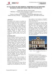
STATISTICAL INTERPRETATION OF THE RESULTS OF BUILDING SIMULATION AND ITS USE IN DESIGN DECISIONS Cristian Ghiaus, Francis Allard LEPTAB, University of La Rochelle, La Rochelle, France

ABSTRACT The practical use of building simulation software requires a global and comprehensible interpretation of results for decision support in design. We propose a method in which the temperature of the free-running building is used to express: 1) the ratio between energy consumption for heating and cooling, 2) energy saved when ventilation is used instead of mechanical cooling, and 3) the degree of building adaptation to the environment. Key words: building simulation, degree-hour, ventilation, free-cooling, energy efficiency.

INTRODUCTION Most of the building simulation programs can solve only closed problems. They respond to a "what happens if" question of the type: what will be the result if this parameter has this value. This is the principle of detailed building simulation programs that are useful for performance evaluation in the final phase of detailed design. They can help the user to estimate the annual energy consumption of the HVAC system of a building but cannot suggest design strategies to improve the building performance. However, in conceptual and preliminary design stages, the problem is open (Beatie and Ward 1999). We need to answer to "what to do" questions such as: Should we design the building to use natural ventilation for cooling or should we consider an air conditioning system? Is it worth to increase the thermal mass? What will be the influence of comfort criteria? How to avoid poor energy performance due to excessive part-load operation of heating or cooling systems? In early stages of design, when architects take decisions that implicitly answer these questions, they have little or no technical support. It is important to have a tool that can respond to an open problem in the conceptual stage of design. This paper presents a method to compare climatic suitability for HVAC systems, including natural ventilation, based on freerunning building temperature. The method is based on statistical interpretation of the results of building

simulation software. This method is appropriate to volume dominated commercial buildings, for which thermal loss due to the air change is much more important than the loss through the building envelope. The method is based on three concepts: the indoor temperature of the free running building, the adaptive comfort, and the frequency distribution of the outdoor air temperature (Ghiaus 2003).

METHOD Balance temperature and the free-running temperature The balance temperature for heating, Tb, is the outdoor temperature for which the building having a specified indoor temperature, Tcl, is in thermal balance with the outdoors. For this temperature, the heat gains (solar, internal) equal the heat losses (ASHRAE 1993):

q gain = K tot (Tcl − Tb ) ,

(1)

where:

q gain

total heat gains [W];

K tot

total heat loss coefficient of the building

[W/K];

Tcl

lower limit of comfort temperature [K];

Tb

balance temperature [K].

The balance point temperature is then:

Tb = Tcl −

q gain K tot

.

(2)

The energy rate needed for heating is:

K tot  (T − To ), if To < Tb q h = ηh b ,  0, if T ≥ T o b  where

- 387 379 -

(3)

ηh

dhc = (1h)(Tcu − T fr )δc ,

is the efficiency of the heating system;

To outdoor temperature.

where

1, if T fr > Tcu δc =  0, if not.

The energy needed for heating is:

Qh = ∫

t fin

t init

with

K tot (Tb − To )δh dt η

1, if To < Tb δh =  0, if not.

.

(4)

i

j

(5)

K tot (i , j ) [Tb (i , j ) − To ( i, j )]δh (6) η( i, j )

Temperature [°C]

(7)

has the dimension degree-hour. The expression (7) has the disadvantage that the balance temperature depends on outdoor temperature and season of the year.

45 Temperatures Tcl lower limit for comfort 40 Tcu upper limit for 35 comfort T fr free-running 30 To outdoor. 25

To Tcu Tcl

20 15

5 0

Heating

Cooling

Ventilation

0 10 20 30 Outdoor temperature [°C]

40

45

(8)

Gains

40

and :

To

30

Tfr Tcu

25

Tcl

35

q gain K tot

.

(9)

By replacing Tb in equation (7) by the expression (2) and considering the equation (9), we obtain an equivalent expression for degree-hours:

dhh = (1h)(Tcl − T fr )δh

20 15 10

(10) 5

and for :

1, if T fr < Tcl δh =  .  0, if not.

Temperature [°C]

T fr = To +

Tfr

Free cooling

10

We can demonstrate that the degree-hours as used in bin method (ASHRAE 1993), can have an equivalent expression in function of the free-running temperature, Tfr, which represents the indoor temperature when no HVAC system is used. By "system" we mean heating, air conditioning and ventilation for cooling. We obtain:

K tot (T fr − To ) − q gain = 0 ,

(13)

It is argued that in naturally ventilated buildings thermal comfort has larger seasonal differences in occupant requirements than assumed by ISO 7730 and ASHRAE 55 Standards (Brager and de Deer 1998), (de Dear, Brager and Cooper 1997), (Nicol and Humphreys 2002). Although the values are controversial, the thermal comfort exhibits a zone delimited by a lower, Tcl, and an upper comfort limit, Tcu; these limits vary with the outdoor temperature (Figure 1).

where summation indexes i and j refer to time interval (e.g. number of hours) and bins of the outdoor temperature, To, respectively. If the time interval is one hour, the factor:

dhh ≡ (1h )(Tb − To )δh ,

.

Adaptive comfort

The total heat loss coefficient of the building and the efficiency of the heating system are a function of outdoor temperature and time. The discrete equivalent of the integral (4) is:

Qh = ∑∑

(12)

Heating

Ventilation Cooling

0 0

(11)

10

20

30

40

Outdoor temperature [°C]

Figure 1 Ranges for heating, ventilation and cooling when the free-running temperature is

Degree-hours for cooling have a similar expression:

- 388 380 -

a) higher and b) lower than the outdoor

Time 12h

Time 18h

To Tfr Tc Tcl

40

Temperature

temperature.

20

20

0

0

Temperature Distribution

0

10

20

30

40

40

40

20

20

0

0

10

20

30

40

0

10

20

30

40

0 0

10

20

30

40

150

Degree - hour

To Tfr Tc Tcl

40

150

100

100

50

50

0

Heating Ventilation Cooling

0 0

10

20

30

40

0

10

Outdoor Temperature [°C]

20

30

40

Outdoor Temperature [°C]

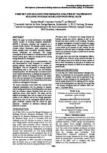
Figure 2 Interpretation of simulation results for12h and 18h: a) Free-running temperature. b) Outdoor temperature distribution. c) Degree-hour for heating, ventilation and cooling.

temperature as a function of the outdoor temperature are, respectively:

Building adaptability If we refer only to the thermal comfort aspect of a building, the aim of the couple formed by the building and the HVAC system is to maintain the indoor temperature within the comfort limits. The difference between the free-running and the outdoor temperature is a measure of the building adaptability. Conceptually, the building may be considered a lowpass filter that damps and lags the outdoor temperature. If there are no gains, the mean values of the indoor and outdoor temperatures are equal. The internal gains increase the indoor temperature mean and also the importance of ventilation for building adaptation. The degree of building adaptability may be expressed as the difference between the free-running temperature and the comfort temperature. The relation between the free-running and the outdoor temperature is not one-to-one (Figure 2). The frequency distribution of degree-hours (for heating, ventilation and cooling) and of free-running

DH h (To ) = (1h)∑ [Tcl (To ) − T fr (To )]δh , (14) T fr

DH h (To ) = (1h) ∑ [T fr (To ) − Tcu (To )]δc (15) T fr

and

DH fc (To ) = (1h) ∑ [T fr (To ) − Tcu (To )]δ fc (16) T fr

where Tfr(To), Tcl(To), Tcu(To) represent the free-running temperature and the comfort temperatures (the lower and the upper limit) that correspond to a bin centred around To;

∑ [•] is the sum for all the values in the T fr

bin centred around To (ASHRAE 1993). The free-running temperature indicates at a glance the degree of building adaptability. Moving the free-

- 389 381 -

running temperature closer to horizontal increases the adaptability. A perfect adaptability would be attained when the slope of the free-running temperature would be zero. A slope larger than π / 4 shows a very bad adaptability, worse than a building with no gains.

STATISTICAL INTERPRETATION OF SIMULATION RESULTS Usually, the results of building simulation are presented as time series of temperatures or heat fluxes. This form is very useful for verifying the design. But building simulation may be also used to propose design solutions. An overview of the building behaviour is given by representations that show simultaneously (Figure 2): •

the free-running temperature,

•

the comfort domain,

• the frequency distribution of the outdoor temperature. Figure 2 (a) presents the results for midday. The first panel shows the building adaptation to the climate. During the cold season, the solar gains are more important due to lower sun angle. During the summer, the sun gains are lesser due to the shading. The angle of the free-running temperature is smaller than π / 4 , showing the adaptation. The second panel shows the distribution of the outdoor temperature and the third the distribution of degree-hours. We note that freecooling by ventilation cannot be used at midday. The free-running temperature is lower than the outdoor temperature due to the thermal inertia. Figure 2 (b) shows a different picture. In the first panel, we can see that at 18h, for near the whole outdoor temperature range, the free-running temperature is higher than the outdoor temperature. In this case, ventilation is a viable solution for freecooling. In the third panel, we note that the energy that could be saved by using ventilation instead of mechanical cooling is about 20%.

CONCLUSIONS The free-running temperature may be used instead the base temperature to define the degree-hours in the bin method. The two definitions are equivalent, but the use of the free-running temperature has the advantage of including the adaptive comfort in the analysis. Another benefit is that the adaptability of the building may be easily visualised. The slope of the free-running temperature shows the building adaptability: smaller the slope, larger the adaptability. A slope higher than π / 4 shows a bad adaptability.

building adaptability. Free-cooling by ventilation becomes more attractive with the increase of internal gains. The method also shows at a glance if it is worth the effort to try to increase the adaptability by ventilation. The frequency distribution of temperature and the direct calculation of degree-hour distribution allow us to assess the importance of changes before these are performed.

AKNOWLEDGEMENTS This work was partly supported by the European Regional Development Fund (ERDF) and partly by the European Commission through the financing of the European project URBVENT in the 5th Fifth RTD Framework Programme.

REFERENCES ASHRAE. 1993. ASHRAE Handbook Fundamentals . Atlanta, ASHRAE. Beatie, K. H., Ward, I.C. 1999. The advantages of building simulation for building design engineers. Building Simulation 99, Kyoto, Japan. Brager, G., de Dear, R. 1998. “Thermal adaptation in the built environment: a literature review.” Energy and Buildings 27: 83-96. de Dear, R., Brager, G., Cooper, D. 1997. Developing an Adaptive Model of Thermal Comfort and Preference, final report ASHRAE RP884, American Society of Heating, Refrigerating and Air Conditioning Engineers, Inc., and Macquarie Research, Ltd. Ghiaus, C. 2003. “Free-running building temperature and HVAC climatic suitability.” Energy and Buildings 35(4): 405-411. Nicol, F., Humphreys, M.A. 2002. “Adaptive thermal comfort and sustainable thermal standards for buildings.” Energy and Buildings 34(6): 563-572.

The free-running temperature also indicates if ventilation is a satisfactory solution for increasing the

- 390 382 -