1022
OPTICS LETTERS / Vol. 29, No. 9 / May 1, 2004
Statistical-mechanics theory of active mode locking with noise Ariel Gordon and Baruch Fischer Department of Electrical Engineering, Technion – Israel Institute of Technology, Haifa 32000, Israel Received August 13, 2003 Actively mode-locked lasers with noise are studied employing statistical mechanics. A mapping of the system to the spherical model (related to the Ising model) of ferromagnets in one dimension that has an exact solution is established. It gives basic features, such as analytical expressions for the correlation function between modes, and the widths and shapes of the pulses [different from the Kuizenga – Siegman expression; IEEE J. Quantum Electron. QE-6, 803 (1970)] and reveals the susceptibility to noise of mode ordering compared with passive mode locking. © 2004 Optical Society of America OCIS codes: 140.4050, 000.6590, 140.3430.
Many mode lasers can operate in two basic regimes: mode locked and not mode locked, where “mode locked” means that the phases of the different axial modes are aligned with one another. When the modes are locked the laser produces pulses. To give rise to such an alignment, interaction between the modes is required. Interaction can be present either as a result of driving (modulation) or by nonlinearity. These indeed are the two classes of technique that are used for mode locking: active and passive, respectively. There are several other differences between the active and the passive techniques. The latter are known to be capable of producing shorter pulses. This fact is usually attributed to the Kuizenga–Siegman 1 theorem of the duration of an actively mode-locked pulse. They give a limit on the pulse width that stems from the balance between production of sidebands by modulation (coinciding with the axial modes) and attenuation of the sidebands by the f iltering action of the laser medium. This limitation indicates some sort of fragility of the active mode-locking process. During each round trip the modulator builds only a small number of neighboring sidebands about every mode. For the sidebands to reach from a mode, say, at the middle of the band to its edges, a large number of round trips is needed, and meanwhile losses suppress the modes at the edge. The fragility of active mode locking lies at the heart of this Letter. We consider susceptibility to something other than losses, i.e., to noise. In the frequency (mode) domain when noise is present, each time sidebands are produced by the modulation, noise slightly alters them. Because these noise-induced errors accumulate as the modulation propagates across the band, correlation across the spectrum cannot be maintained beyond a certain distance, which is determined by the modulation strength and the level of noise. As only statistically correlated modes can add constructively to a pulse, the width of the pulses will be inversely proportional to this spectral correlation length rather than to the spectral width. Here we follow a statistical-mechanics approach to the study of many interacting modes (our particles) in a passive mode-locked laser system with noise2 – 4 and apply it to the active case. First we show that the distribution of the mode amplitudes in active mode locking is exactly given by a Gibbs-like distribution, as we found for the passive case. This opens the 0146-9592/04/091022-03$15.00/0
way for employing the mature and sophisticated tools of equilibrium statistical mechanics. Then we show an exact mapping of the actively mode-locked laser onto the spherical (or the infinite spin dimensionality) model of ferromagnets,5,6 which models a ferromagnet as a system of nearest-neighbor interacting spins and is a slight modification of the better-known Ising model. These magnetic systems have an exact solution in one dimension. In the case of the laser, spins are replaced by mode phasors; interaction by modulation, which induces the formation of neighboring sidebands (modes); and temperature by noise. Then we immediately have a complete description of the mode system’s behavior by means of an exact mathematical solution of the one-dimensional spin system. It gives, for example, expressions for the noise-dependent correlation between modes, and the average shape and width of the pulses. With the statistical-mechanics approach the difference between active and passive mode locking is obvious. It is embedded in the range of the interaction between modes. For the short-range interaction of the active case, as the modulation strength (interaction) becomes weaker compared with noise (temperature), the correlation length becomes shorter, the islands (clusters) within which modes can coherently add up to a pulse become smaller, and the pulse becomes wider (see Fig. 1). Here a phase transition to a fully ordered state (magnetization) occurs in principle only at zero noise (because the number of modes is f inite, this picture is precise when the spectral correlation length is shorter than the finite bandwidth). The fragility of active mode locking then becomes simply another instance of the well-known lack of magnetization (overall ordering) of one-dimensional short-range-interacting spin systems: Any weak noise (temperature) in the mode system can easily break a bond between neighboring modes, thus eliminating overall mode ordering. In contrast, the long-range interaction in passive mode locking by four-wave mixing in the saturable absorber imposes overall order below a certain noise level (with only slight perturbations owing to noise7) and complete disorder above it, resulting in the threshold behavior of the passive mode locking: As all modes interact almost equally with all others, once the interaction through the many mode – mode bonds is strong enough to overcome noise it induces correlation © 2004 Optical Society of America
May 1, 2004 / Vol. 29, No. 9 / OPTICS LETTERS
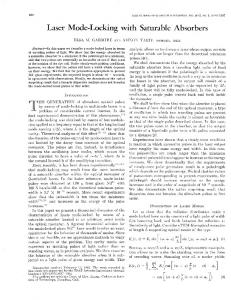
Fig. 1. Axial mode system in the frequency (n) domain, where the arrows describe the mode amplitudes and phases (phasors) and the corresponding one-period light-intensity prof iles in the time domain (tR is the cavity round-trip time). Note the resemblance to the magnetic spin system, where the arrows describe spins. The traces at the right are given for various ordering levels, from (top to bottom) complete disorder, through partial order with a finite correlation length, to a highly ordered and then to a completely ordered state. The degree of order is determined by AP0 兾W .
1023
the instantaneous total intracavity power. Although the precise form of gain saturation function g共P 兲 is immaterial to our calculation as long as it is slow, we take the common g共P 兲 苷 g0 兾共1 1 P 兾Psat 兲 model, where g0 and Psat characterize the small-signal gain and the saturation power of the amplif ier, respectively, l is the total intracavity loss, and A is the modulation strength. Different interpretations exist that lead to an equation of the same structure.8 Gm is a complex white Gaussian-noise term, which represents spontaneous emission noise or otherwise satisf ies 具Gm 共t1 兲Gn ⴱ 共t2 兲典 苷 2T dmn d共t1 2 t2 兲, where the constant T characterizes the power of the noise and 具 典 denotes an ensemble average. We assume that the amplif ier supports N modes, a1 . . . aN , and for convenience we induce periodic boundary conditions. This means that in Eq. (1) for m 苷 1 and m 苷 N we have aN and a1 instead of a0 and aN 11, respectively. Because of the short-range interaction induced by the modulator, such a change in the boundary condition will not affect the system. Defining A HI 苷 2 J 2 g0 Psat ln共Psat 1 P 兲 1 lP , 2 X J 苷 共am am11 ⴱ 1 am ⴱ am11 兲 ,
(2)
m
one can rewrite Eq. (1) as all over the band. All the modes in the band stay together and all can be ordered, leading to a sharp noiseinduced threshold behavior with a clear separation between locked and unlocked thermodynamic phases.2 The spin– spin correlation function is one of the most interesting aspects of phase transition theory, because it is directly measurable by, for example, neutron scattering experiments. It turns out that this function is also most simply measured for lasers: The Fourier transform of the mode – mode correlation is the average intensity prof ile of the pulses at the output of the laser. Using this correlation function, we compute the average intensity prof ile and in particular the pulse width as a function of the noise-to-signal ratio and the modulation strength. We shall show that, for long lasers, even quantum noise can impose a lower limit on the pulse width that may dominate the Kuizenga– Siegman limit. The laser system that we consider consists of an amplitude modulator, a slow (compared with the laser round-trip time) saturable amplifier, and a spectral f ilter. Here we consider a rectangular prof ile of spectral filtering: f lat within some band and rapidly dropping to infinite loss outside. Another commonly made approximation for the gain prof ile is parabolic, a condition that we do not treat further here. The equation of motion then takes the form aᠨ m 苷 共A兾2兲 共am21 1 am11 兲 1 关g共P 兲 2 l兴am 1 Gm ,
(1)
where am are the complex amplitudes of the axial modes of the laser. The electric field is expanded to its spatial Fourier components am at every instant, so aᠨ m denotes the temporal each am is a function of time. P derivative of am . P 苷 m am am ⴱ is (proportional to)
aᠨ m 苷 2
≠HI 1 Gm , ≠am ⴱ
aᠨ m ⴱ 苷 2
≠HI 1 Gm ⴱ . ≠am
Similarly to what was reported in Ref. 2, the latter equation can be split into a real part and an imaginary part to better reveal that the equations satisfy the potential condition.9 The steady-state distribution of the a’s is therefore ∂ µ HI r共a1 , . . . aN 兲 ~ exp 2 T ∏ ∑ g0 Psat ln共Psat 1 P 兲 2 lP 苷 exp T ∂ µ AJ . 3 exp (3) 2T This is a central result, rigorously showing that our mode system obeys Gibbs-like statistics (as we have shown for passive mode locking2 – 4). Here HI and T play the role of the Hamiltonian and temperature, respectively, in statistical mechanics. We perform our statistical-mechanics analysis in the thermodynamic limit, i.e., when the number of modes approaches infinity. In fact, 50– 100 modes already make the system large, as long as the restriction made in inequality (8) below on the correlation length is fulfilled. We assume that, although the number of modes increases, intracavity power P and the total power of noise W 苷 2NT remain constant. It is evident from relation (3) that the term exp共AJ 兾2T 兲 provides the interaction between the modes that is due to modulation, whereas the other term on the right-hand side of relation (3) stabilizes
1024
OPTICS LETTERS / Vol. 29, No. 9 / May 1, 2004
larger than the total size of the spectrum; in other words, all the modes in the spectrum are correlated. When Ncor .. N, that is, when W ,, AP0 兾N , the theory reduces to the noiseless case. The other variation, the target of our present study, is Ncor , N: W . 2AP0 兾N .
(8)
The average intensity of the electric f ield in the laser is then given by 具jc共t兲j2 典 苷
X
具am an ⴱ 典exp关2pi共m 2 n兲t兾tR 兴
m, n
苷
Fig. 2. Average pulse intensity prof iles [Eq. (9)], showing one period, for various correlation lengths.
power P about some constant value, roughly equal to P0 苷 Psat 共g0 兾l 2 1兲. Here we claim, as we did in Refs. 2 –4, that the details of this stabilizing mechanism are immaterial as long as the gain saturation remains slow, and it can be replaced by the constraint P 苷 P0 . Anyway, in the thermodynamic limit exp兵关g0 Psat ln共Psat 1 P 兲 2 lP 兴兾T 其 approaches (up to a coefficient) d共P 2 P0 兲. We therefore approximate distribution (3) by ∂ µ AN J . (4) r共a1 , . . . aN 兲 ~ d共P 2 P0 兲exp W Relation (4) establishes the mapping of actively modelocked lasers to the spherical p model of ferromagnets.5 To see this, we def ine a˜ m 苷 NP0 am , and in terms of a˜ m relation (4) is exactly the distribution given in Ref. 5 for one dimension, except that the spins (modes) are complex rather than real. For real spins the spin correlation function in the one-dimensional spherical model is given, for example, in Ref. 10. Repeating the calculation in Ref. 5 with complex spins, one can find the same result apart from a factor of 2: For complex spins the interaction coefficient is effectively twice weaker. This correlation function is exponentially decaying and has the form Ω æn 2AP0 兾W P0 . (5) 具ak ak1n ⴱ 典 苷 N 1 1 关1 1 共2AP0 兾W 兲2 兴1兾2 For lasers the case of interest occurs when noise has a much smaller magnitude than the signal, W ,, AP0 , in which case Eq. (5) simplifies to yield µ ∂ ∂ µ W n P0 P0 2nW . ⴱ 12 具ak ak1n 典 艐 艐 exp (6) N 2AP0 N 2AP0 Relation (6) reveals the average mode cluster size (the correlation length): 2AP0 . (7) W We can now identify the two possible operation regimes of the system: In the f irst, the correlation length is Ncor 苷
P0 , 2 2AP0 cos共2pt兾tR 兲兾W
(9) 关1 1 共2AP0 P where c共t兲 苷 am exp共2pimt兾tR 兲 is the slowly varying amplitude of the electric field, tR is the cavity round-trip time, and Eq. (5) has been used. This is a Lorenzian prof ile (see Fig. 2). Its width (FWHM) is t 艐 tR W 兾共2pAP0 兲. For the small-noise system the intensity prof ile does not reduce in our model to the well-known Gaussian prof ile, as our gain prof ile is rectangular rather than parabolic. Therefore for the noiseless case [the opposite of inequality (8)] the waveform reduces to sin2 共Npt兾tR 兲兾sin2 共pt兾tR 兲. The width of this waveform is of the order of tR 兾N, determined by the size of the band, whereas with noise, in the regime of inequality (8), it is of the order of tR 兾Ncor . Finally, it is interesting to note that a small noise-tosignal ratio can bring the system to a noise-dominated condition [inequality (8)]: A noise-to-signal ratio of 1024 , AtR 苷 0.05, and N . 103 modes are suff icient. Such noise is plausible even for spontaneous emission, and N . 103 is common for long-f iber lasers. Therefore there are cases when quantum noise is enough to reach the noise-dominated regime. 兾W 兲2 兴1兾2
This study was partially supported by the Israel Science Foundation. B. Fischer’s e-mail address is
[email protected]. References 1. D. I. Kuizenga and A. E. Siegman, IEEE J. Quantum Electron. QE-6, 803 (1970). 2. A. Gordon and B. Fischer, Phys. Rev. Lett. 89, 103901 (2002). 3. A. Gordon and B. Fischer, Opt. Commun. 223, 151 (2003). 4. A. Gordon and B. Fischer, Opt. Lett. 18, 1326 (2003). 5. T. H. Berlin and M. Kac, Phys. Rev. 86, 821 (1952). 6. H. E. Stanley, Introduction to Phase Transitions and Critical Phenomena (Oxford U. Press, Oxford, UK, 1971). 7. H. A. Haus and A. Mecozzi, IEEE J. Quantum Electron. 29, 983 (1993). 8. H. A. Haus, IEEE J. Sel. Top. Quantum Electron. 6, 1173 (2000). 9. H. Risken, The Fokker –Planck Equation, 2nd ed. (Springer-Verlag, Berlin, 1989). 10. H. E. Stanley, Phys. Rev. 179, 570 (1969).