orbiter, and the Mariner 10 Venus-Mercury space probe where noisy information about the satellite (such as ...... Write this last formulation as v = 08 + e. Then the ...
NUREG/CR-0683 PNL-2920
STATISTICAL METHODS FOR EVALUATING SEQUENTIAL MATERIAL BALANCE DATA
M. A. Wincek K. B. Stewart G. F. Piepel Pacific Northwest Laboratory Richland, WA 99352
Prepared for
U. S. Nuclear Regulatory Commission
NOTICE This report was prepared as an account of work sponsored by an agency of the United States Government. Neither the United States Government nor any agency thereof, or any of their employees, makes any warranty, expressed or implied , or assumes any legal liability or responsibility for any third party's use, or the results of such use, of any information, apparatus product or process disclosed in this report, or represents that its use by such third party would not infringe privately owned rights.
Available from National Technical Information Service Springfield, Virginia 22161 Price: Printed Copy $9.00 ; Microfiche $3.00 The price of this document for requesters outside of the North American Continent can be obtained from the National Technical Information Service.
-
,
TABLE OF CONTENTS iii
LI ST OF FIGURES
v
LIST OF TABLES .
vii
EXECUTIVE SUMMARY 1.0
INTRODUCTION
2.0 RECURSIVE AND NON-RECURSIVE METHODS FOR DETECTING INVENTORY DIFFERENCES IN NO-LOSS MODELS 2. 1 THE FUNDAMENTAL MODEL 2.2 THE MUF MODEL 2.3
....
THE CUMULATIVE MUF MODEL
2.4 STEWART'S WEIGHTED ESTIMATES MODEL
5 5 6 9 13
2.4.1
Some Observations on the Results
16
2.4.2
Smoothed Estimates
24
2.5 THE STATE VARIABLE APPROACH
26
2.6 THE RECURSIVE REGRESSION MODEL
39
SUMMARY OF THE NO- LOSS MODELS
41
2.7. 1 Weighted to Unweighted Regression
42
3.0 MINIMUM VARIANCE UNBIASED ESTIMATES OF LOSS AND INVENTORY AMOUNTS . . . . . . . .
47
2.7
3. 1
SOME LEAST SQUARES APPROACHES TO SEQUENCES OF MUF s AND I NVENTORY VALUES . . . . . .
48
3. 1 . 1 Approach 1: An Overa 11 Least Squares Solution That Requires Only Standard Least Squares Computer Programs
50
3.1.2 Approach 2: MUF's as Dependent Variables, a Full Scale Generalized Least Squares Approach
52
I
3.1.3 Approach 3:
A Recursive Solution
53
3. 1.4 Approach 4:
Recursive Estimation Without Matrices
55
3. 1.5 Approach 5:
An Approach Based on Sume Previous Results
57
TABLE OF CONTENTS (contd.) 3.2
THE MVUE WITHOUT A LOSS TERM IN THE MODEL 3.2.1
3.3
59
The Effects of Measurement Bias for the No-Loss Term Situation . . .
61
THE INTRINSIC INFORMATION IN A SEQUENCE OF MUF's AND INVENTORY MEASUREMENTS .
62
A
3.3.1
The Standard Deviation of L(n)
63
A
3.3.2
The Standard Deviation of i(n/n) in the Constant Loss Model . . . . . . . .
65
A
3.3.3 3.3.4
The Standard Deviation of i (n/ n) in the No-Loss Model
67
The Proportional Increase in 0i(n/n) Due to a Loss Term
69 A
3.3.5
3.4
The Effects of a Net Throughput Bias on i(n/n)
71
3.3.6 A Simple Example Comparing the Powers of Different Loss Estimation Techniques
73
MASS BALANCE STATISTICS POWER CURVES
73
4.0
CONCLUSIONS
5.0
TERMINOLOGY AND NOTATION
103
6.0
REFERENCES
105
~
.
99
APPENDIX A:
THE TESTING OF A STATISTICAL HYPOTHESIS
APPENDIX B:
THE V-MASK TECHNIQUE
APPENDIX C:
DERIVATION OF THE RECURSIVE WEIGHTED ESTIMATES APPROACH
APPENDIX D:
DERIVATION OF DISCRETE KALMAN FILTER EQUATIONS
APPENDIX E:
COMPUTER OUTPUT FROM APPROACHES 1-5
ii
LIST OF FIGURES Page
No. The Basic State Variable Model
27
2
The Basic State Variable Model with Noise
27
3
The MUF Situation
4
Power Curves for n=2, c=O.Ol
77
5
Power Curves for n=5, c=O.Ol
78
6
Power Curves for n=10, c=O.Ol
79
7
Power Curves for n=20, c=O.Ol
80
8
Power Curves for n=2, c=O.l
81
9
Power Curves for n=5, c=O.l
82
10
Power Curves for n=10, c=O.l
83
11
Power Curves for n=20, c=O.l
84
12
Power Curves for n=2, c=0.5
85
13
Power Curves for n=5, c=0.5
86
14
Power Curves for n=10, c=0.5
87
15
Power Curves for n=20, c=0.5
88
16
Power Curves for n=2, c=1. 0
89
17
Power Curves for n=5, c=1. 0
90
18
Power Curves for n=10, c=1.0
91
19
Power Curves for n=20, c=1.0
92
.
27
iii
LIST OF TABLES No. Outline of the Computational Scheme for the Weighted Estimates Model
16
2
Summary of the Computational Aspects of the No-Loss Models
41
3
Th2 Loss Estimate Standard Deviations as Functions of c and Periods . . . • . . .
64
The Ending Inventory Estimate Standard Deviations as Functions of c and Periods
66
The Standard Deviation of the Ending Inventory Estimate with the No-Loss Model
68
The Proportional Increase in the Standard Deviation in Estimating i(n/n) when an Unnecessary Loss Term is Used
70
The Effect of Net ThroughRut Bias in the No-Loss Si.tuation on the MVUE of i(n/n) . . . . . . . . . . . .
72
4
5 6
7
v
EXECUTIVE SUMMARY Present material balance accounting methods focus primarily upon the ma teri a1 unaccounted for (MUF) stati sti c, whi ch util i zes the data from only one material balance period as an indicator of a possible loss of nuclear material. Typically a cumulative MUF (CUMUF) statistic, which utilizes all the available f10w data, is also calculated; b~t there is no statutory requirement that it be reported or evaluated. Previous work(5) has shown that cumulative MUF has greater power than MUF to detect small constant losses. Techniques which emphasize the sequential nature of MUF (that is, MUF as a sequence of values related over time) are also expected to be more sensitive for detecting losses. The recursive estimation algorithm known as the Kalman filter has been proposed(3) as a possible solution which uses the above idea. The purpose of this study was to evaluate the application of the Kalman filter to the MUF problem, to propose other approaches to the problem, and to re-examine the traditional MUF and cumulative MUF statistics in more general settings. ll
II
The report considers the material balance model where the only modeled variability is that due to the measurements of the net throughput (inputs minus outputs) and the inventories. The problem discussed is how to extract more information from all the available data. Section 2 considers material balance models which assume no loss, while Section 3 considers the constant loss and a11-at-once loss situations. Emphasis was placed on explaining state variable models and Kalman filtering in relation to the general linear statistical model to which least squares is applied yielding a minimum variance unbiased estimator. All errors affecting material balances were assumed to be random. • The main results of the study are: • The state variable model to which the Kalman filter is applied does not extract any inform"a tion from the data that cannot be obtained by other methods such as the usual statistical least squares. Filtered estimates and smoothed estimates can be obtained from either point of view. The
vii
Kalman filter algorithm is computationally most efficient in producing filtered estimates. Another algorithm must be used in conjunction with the filter to produce smoothed estimates. The least squares approach can be made to produce filtered and smoothed estimates either simultaneously or individually. •
Estimation procedures for models which describe specific loss mechanisms are optimal in those cases where the model is exact. When the true loss mechanism is different from the modeled loss mechanism, the model can give the estimation procedure a low power of detection and can lead to erroneous conclusions.
• All of the loss estimators are most effective in detecting losses when the net throughput and inventory measurement variances are small. The special loss statistics derived from the information in a sequence of accountability periods are the most effective relative to MUF and CUMUF, the traditional loss statistics, when the ratio of the net throughput measurement variance to the measurement variance of the inventory is small. In this favorable situation, the estimator of constant loss does better, but not appreciably better than CUMUF, if the loss amount from period to period is truly constant. The three loss estimators, MUF, CUMUF and the weighted least squares estimate, are relatively easy to calculate and taken as a group have about as much loss detection capability as the measurement system will allow. The above results give the following suggestions for the analysis of material balance accounting data: •
From a mathematical point of view there are many "optimal" techniques for the analysis of material balance data. From a practical point of view, there are none. Each mathematically "optimal" technique can be shown to be non-optimal when the model is incorrectly specified. In particular, specific loss models are optimal only when the exact loss is modeled. An alternative is to form an integrated package of several of these specific model techniques. Although the individual techniques
viii
have well known statistical properties, the integrated package taken as a whole may not (e.g., it may be difficult to calculate the false alarm rate). From a practical viewpoint, the integrated package is to be preferred over a specific technique, since the latter is inadequate in fulfilling the goals of safeguards. This report does not investigate this idea further. • The inclusion of non-random errors in the analysis can be- effectively dealt with if they can be modeled. Since the statistical techniques are well developed, future work should emphasize obtaining better models. This model identification problem is a practical problem and not just a ~tatistical one .
ix
1.0
INTRODUCTION
The principal statistic in material balance accounting is the MUF statistic defined by MUF(k) = z(k-l) + f(k-l) - z(k) where z(k-l) f(k-l) z(k)
is the measured beginning inventory for the kth period; is the measured net throughput for the kth period (k-l,k], the receipts minus removals, which is also called the flow; is the measured ending inventory for the kth period, which is measured beginning inventory for period k+l.
Whether the inventory in the material balance area during period k is under control is decided in part by a comparison of MUF(k) with its associated limit of error. Other work(5) has shown, however, that the total MUF structure can provide a significant extra amount of information about inventory values and losses; cumulative MUF is an example of this. The extension of this idea is the problem of interest in this report. The problem is whether the total information, z(k), k=O, . . . , nand f(k), k=O, ... , n-l, can be used in a joint fashion to obtain an unbiased estimate of the true inventory and any losses which may have occurred with appreciably greater precision than the direct measurements of inventory provide. The choice of an approach for estimating the true inventory and loss depends on the following: •
the statistical models which relate the observed variables with their actual values;
•
knowledge of the variance structure;
•
the desired statistical qualities of the estimation method;
•
the knowledge of the practitioner in the field in applying and interpreting the results of statistical techniques:
•
the computational capability and facilities which are available for the implementation of a statistical procedure;
•
the robustness of the procedure.
Though these criteria are not all simultaneously considered in the actual development of a technique, in the end they will be used to determine if the technique has any practical value. Two conditions determine the practical value of a technique: 1) a technique which is not understood is not likely to be used; and 2) the robustness of a technique (it's insensitivity to deviations from assumptions) is inversely proportional to the number of assumptions. This second point is based on the observation that complicated mathematical models are based on propositions which are assumed to be true. Since the validity of the model and the results obtained from it are dependent on the assumptions, more assumptions create more ways the model can go wrong. Thus, a model based on many assumptions may not be very robust. Work which has addressed the idea of using all the data to determine the material balance status of a period has introduced the Kalman filter as a possible estimation scheme for the material balance data. The Kalman filter has been successfully applied in the Apollo lunar missions, the Mariner 9 Mars orbiter, and the Mariner 10 Venus-Mercury space probe where noisy information about the satellite (such as locat-ion) had to be processed immediately to provide up-to-date estimates of satellite parameters so that proper control could be maintained. The recursive nature of the Kalman filter solved this otherwise impossible estimation problem. The Kalman filter provides minimun variance unbiased estimates of state vectors for a linear model to which (Gauss-Markov) least squares is applied also produces minimum variance unbiased estimators. This report compares the two approaches to determine if one approach provides any more information than the other. The current methods of dealing with MUF can be classified into two categories: •
"non-least squares" methods, e.g., MUF, cumulative MUF;
2
• "least squares" methods,(a) e.g., regression methods, Kalman filter. Comparison of the two categories reveals the following points: Non -Least Squares Methods •
are based on simple models with a minimum of detail and assumptions;
•
involve rather basic statistics;
•
assume no specific loss mechanism;
•
are used primarily to detect loss, but not to estimate the amount lost;
•
may use only the most recent data (e.g., MUF) or may use all the data (e.g., cumulative MUF);
•
do not minimize variance subject to the constraint of unbiasedness.
.
Least Squares Methods •
are based on models containing more details and assumptions;
•
involve more complicated statistics;
•
may assume a specific loss mechanism;
•
are used to detect loss and, in those cases where a specific loss is modeled, to estimate the amount of loss;
•
use all the data to arrive at the current estimate (of inventory, loss, ' or whatever is considered in the model);
•
produce linear estimates of inventory which have minimum variance and are unbiased. (b)
Because the least squares methods are more specific, they perform better than the non-least squares methods in those cases where the least squares models are exact. On the other hand, use of a least squares method for an (a)In this report the weighting matrix of the least squares performance criterion is the inverse of an appropriate covariance matrix so that the least squares estimator is the same as the linear minimum variance estimator. (b)A linear estimator which has minimum variance and is unbiased is referred to as a linear MVUE.
3
incorrectly modeled situation can give poor results. For example, a simple constant loss model has less power to detect an all-at-once (block) loss than MUF. The second section defines the material balance situation by a fundamental model and then proceeds to give alternative models which are transformations of the fundamental model. Methods for producing linear minimum variance unbiased estimates of inventory are also discussed with respect to the relevant models. In particular, state variable models of the material balance situation with recursive (Kalman filter) and non-recursive estimation are also discussed. All models assume that there is no loss and that all errors are random. The third section extends the ideas of Section 2 to include models which describe a constant loss. The performances of th~ no loss models of Section 2 and the constant loss models of Section 3 are evaluated by power curves for the cases of an all-at-qnce loss and for a constant loss. The power curves graphically summarize the major conclusions of the report.
4
2.0 RECURSIVE AND NON-RECURSIVE METHODS FOR DETECTING INVENTORY DIFFERENCES IN NO-LOSS MODELS 2.1
THE FUNDAMENTAL MODEL
A fundamental model for the particular material balance situation of concern in this report may be written by putting all the observed variables on one side of the equation and all the system parameters on the other side premultiplied by a design matrix which links the observables to the parameters. To account for random error in measurement, error variables are also added. The model for n periods can then be written as follows: ( n+ 1) x (n+ 1 )
z(O)
1
o0
z( 1)
0
1 0
. =
v( 1) i( 0) i ( 1)
,
o1 o0 o0
0
o -1
v(O)
,
o -0 - 0 -1
f(n-l
o0 ... o 0
1
+
i(n
-1
000
w( n-1)
(n+ 1)
n x
with a covariance matrix assumed to be
R(O)
o
0
0 R( 1)
0
0 0
0
.
,
o o
0
10 10
_
'..!..'
I: , I' ~(nlIO_ - - 0 o I Q(O) ... 0 I:
o
0
0
10
Q(n-1)
I
5
where z(k)
_ the measured ending inventory for material balance period k (k-l, k]
f(k-l)
_ the measured receipts minus removals for material balance k = the flow = net throughput
i(k)
= the true ending inventory for material balance period k
u(k-l)
= the true flow for material balance period k
v(k)
=
the inventory measurement random error variable with variance R(k)
w(k)
=
the flow measurment random error variable with variance Q(k).
The model is called "fundamental" because it relates all the observables, inventory measurements and flow measurements, to the actual inventory values when no loss is occurring. 2.2 THE MUF MODEL The book physical inventory difference is the difference between the book inventory (the material which is supposed to be present) and the physical inventory (the material which is actually measured). The inventory difference can be expressed as MUF(k)
=
z(k-l) + f(k-l)
z(k)
=
i(k-l) + u(k-l)
i(k) + v(k-l) + w(k-l) - v(k)
At k, the values MUF(l), ... , MUF(k) can be concisely expressed in matrix notation as a linear transformation of the fundamental model:
6
MUF k :: MUF(l)
=
MUF(k)
1 -1 0 0 1 -1
0
0
0
0
oI 1
0
010
I I 1 -1 I
n x (n+ 1)
0
0
z(O) z( 1)
1
~C!5.)_
0
0
0
-
nx n
f(O) f( 1)
f(k-1) i( 0)
1 -1 o ... 0 0 1 -1 ... 0
= 0
0
oI10 o I o1 I I o ... 1 - 1 I o 0
... 0
i (1)
... 0
i( 2)
+ ... 1
iC~J_
u(O) u(1)
u (k- 1)
where
e( 1)
e(2)
e( k)
=
v(O) + w(O) - v(l) v(l) + w(l) - v(2)
v(k-1)+w(k-1)-v(k)
7
e( 1)
e(k)
with covariance matrix, 1 -1 0 0 -1
0 0 0
0 0 11 0 0 0 10 1 I·... I' . -1 10 0
~
MUF k
o
=
R(O)
o
o
...
0 10 1. 1 R(k)1 0
0
0
. .. 0
o -1
0 0 0
0 0 0 0 - - 0 0
1 -1 -0 0
--------------
1
0
0 IQ(O)
0
1 . 1 0 0 ... Q( k-l 1
0
o
=
R(O)+R(l)+Q(O) -R(l) 0 -R(l) R(1)+R(2)+Q(1) -R(2) o -R(2) R(2)+R(3)+Q(2)
o
o
o
o o o
-
0
o o
o
... -R(k-l) R(k-l)+R(k)+Q(k-l)
The interpretation of this matrix is that the (i,i) diagonal element is the variance of MUF(i) and the (i ,i+l) and (i+l,i) elements are the covariance of MUF(i) and MUF(i+l). Note that the covariance of successive values is negative. Under the hypothesis of no loss, the expected value of MUF is zero . The realized MUF value is compared with LEMUF (twice the standard deviation of MUF) to see if the non-zero value of MUF can be explained by measurement noise. If it cannot, then there is an indication that the MUF model is inadequate. The inadequacy of the model may be due, for example, to incorrectly stated variances or unmodeled losses. Use of the MUF model involves no estimation procedures.
8
2.3 THE CUMULATIVE MUF MODEL Cumulative MUF is simply i
CUMUF( k) -
L
MUF( i)
i =1
which
{~
an inner product in matrix notation: CUMUF(k) = (1 ... 1)
MUF(1)
MUF(k)
= -4< lT ~ MUF
,
where ~ is the column vector of k 1 's. At n, the values CUMUF(l), ... , CUMUF(n) can be expressed as a linear transformation of the MUF model: CUMUF(l) CUMUF(2)
1
0
= 1
0
o
0
o
MUF(l) MUF( 2)
CUMUF(n)
MUF(n
which is a linear transformation of the fundamental model:
CUMUF( 1) 1 -1 0 CUMUF(2) = 1 0 -1
0
1
0
0
0
0
z(O) z( 1) z(2)
~(.D)_
CUMUF(n
0
0
-1
1
1
f(O) f( 1) f(2)
f(n-1)
9
; (0)
1 -1
a
a -1 =
a
0
aI aI . II . 1 -1 I
a a a
a a
; (1) ;(2)
1
iCIJ)_ u(O) u(1)
(n-1 1 -1 0 1 0 -1
I1 I1 I . I I
0 0
+ 0
0
-1
0
0
0
1
0
0
v(O) v( 1) v(2)
1-
~C~~J_
w(O) w( 1)
w( n- 1 L
The covariance ables is: -1
matrix,~CUMUFn'
o o ... a o ... 0 1
0 ... 0
o -1
of the transformed measurement random vari-
0
R(O)
0
I I I
0
0
-1
_o_ _.~._Rlnll _ Q ~.~Q o
0 ... -1
1
o
1
0
0
o -1
0
o 0
-1
0 IQ(O) ••• 0
I
o
1 1
0
I 0 I
1 ...
Q(n-1)
o o
1
0
o 0
10
R(O)+R(l)+Q(O) R(O)+Q(O) R(O)+Q(O)
=
R(O)+Q(O)
... R( 0 )+Q( 0) 1 1 R(0)+R(2)+ ~Q(i) ..• R(O)+l~Q(i) 1 1=0 2 R(O)+:E Q(;) ... R(O)+L:Q(;) ;=0 ;=0
R(O)+Q(O) R(O)+
i Q(;)
;=0
R(O)+ tQ(i) ;=0
... R(O)+
R(O)+ tQ(i) ;=0
k . .• R( 0) +R( k+ 1) + :E Q( ;) R( 0 ) + :E Q( i) ;=0 ;=0
R(O)+Q(O)
R(O)+ ±Q( i) ;=0
... R(O)+ ~ Q(i) ;=0
R(O)+Q(O)
R(O)+ tQ(i) ;=0
... R(O)+ ~ Q(i) ;=0
:E Q(;)
;=0
.
·· · k
R(O)+Q(O) 1
... R(O)+Q(O) 1 •.. R(O)+ L:Q(i) ;=0
~ Q(i) ;=0 k+l k+1 R(0)+R(k+2)+ :EQ(;) ... R(O)+ L:Q(i) ;=0 1=0 '"
R(O)+
--' --'
R(O)+kI:Q(i) ;=0
n-1 ... R(O)+R(n)+~Q(;) ;=0
The covariance matrix points out that all CUMUF values are correlated with each other, in contrast to MUF where only successive values are correlated. The matrix also shows that k
Var [CUMUF(k+l)]
= R(O) + R(k+l) +
L
Q(i).
i=O
k
If
L
Q(i), the variance of the flow, is denoted as Q*(k), then
i=O Var [CUMUF(k+l)]
= R(O) + R(k+l) + Q*(k)
which in words is variance of the ) ( beginning inventory
+
vari ance of the) ( ending inventory
+
variance of the) ( flow
This is exactly the same form . as the variance of a single MUF except that for MUF the beginning inventory is at k, instead of 0, and the variance of the flow is Q(k), instead of Q*(k). Thus, cumulative MUF is exactly equivalent to MUF except for the timt span. The person who calculates cumulative MUF at time k+l from individual MUF's obtains the same answer as the person who calculates a single MUF over the period [O,k+l] without calculating the individual MUF's. The latter would call the calculated quantity MUF while the former would call the quantity cumulative MUF. Just as with MUF, the expected value of CUMUF is zero under the hypothesis of no loss. The realized value of CUMUF is compared with twice its standard deviation to see if the non-zero value can be explained by measurement noise. No estimation procedure is involved in the CUMUF statistic.
12
2.4 STEWART'S WEIGHTED ESTIMATES MODEL At the end of an arbitrary material balance period n, there are n+l estimates of the current inventory: z{O) + f{O) + f{l) + ... + f{n-2) + f{n-l) z{l) + f{l) + ... + f{n-2) + f{n-l) z{n-1) + f{n-l) z{n) 0
0
0
0
0
1 1
1
0
0
0
0
. · ··
=
1 1
z{O) z{ 1)
z{n-2) z{n-l)
0
0
0
1 0
0
0
0
1
0
0
0
0
0
0
0
0
~(!l) __
f{O) f{ 1)
f{n-2) f{ n-1)
o ...
1 0
=
0
0
0
1
0
0
0
0
0
1 0 0 1
0 0
1 1 1 1
v{O) v{ 1)
0
0
o •..
0
v{n-2) v(n-1)
i{n) + : 0 0
o . .. o ...
0
0
~(!l)_
w{O) w{ 1)
w{n-2) w{n-l 13
with covariance matrix, 1 0 0
000 11 1 000 10 1
o 0 o 0
I· .. I· 010 10 0 o 0 1 10 0
0 R{ 0) 0 ... 0 I 0 0 0 R{ 1) ... 0 I 0 I . I _O__O_~.~Rinll_o_ _ .~. __0_ o 0 ... 0 IQ(O) ... 0
1
0
0
I 0 I 0
0
... Q{n-l)
1 0 o1
o 0 o 0
o 0 o 0 10 o 0 o -1 -o -0 - - 1 0 o 0 1 o 0
0 n-l
n-l R{O) + n-l
2:
i=l = n-l
2:
i=2
2:
i=O
Q(i)
2:
n-l
2:
Q( i)
'i=2
i =1 R(1) +
2:
i -1
2:
Q( i)
k=2
n-l Q( i)
2:
i=2
Q(n-l)
o
o
0
Q( i)
... Q(n-l)
0
...
0
R(2) +
Q{ i)
Q{n-l)
Q(n-l)
n-l
n-l Q(i)
Q( i)
n-l
2:
i=2
Q( i)
Q{n-l)
R(n-l) + Q(n-l) 0
Q(n-l)
o denoted ~n'
o
R(n
If the above covar i ance matrix is then the linear minimum variance unbiased estimator of the inventory i(n) which uses all the available information up to and including period n is given by A
'"" -1
i{n/ n) - (1'L.J n
14
-1)
-1
,",,-1 l'L.J n
Yn
where 1 is a vector of n+l lis, and
z(O) y n
= z(n)
T(O) -
f(n-1) Stewart(4,8) developed the idea for the estimator and put it into recursive form . Appendix C gives the details of the derivation. The following notation is employed: A
i(k+l/k+l)
_ the lineai minimum variance unbiased estimator of the inventory at period k+l after the measurement of the physical inventory z(k+l) has been made
A
i(k+l/k)
-
the linear minimum variance unbiased estimator of the inventory at period k+l after the ' flow f(k) is known but before the physical inventory has been made
K(k+l)
-
the last element in the row vector (1'~ which multiplies z(n+l) n
-l
1)
-1
-1 1'~
P(k+l/k+l)
_ the variance of the estimate -of inventory at time k+l given measurements up to and including time k+l
P(k+l/k)
-
n
variance of the estimate of inventory for time k+l given measurements up to and including time k
Given the above definitions, the recursive relations can be written as foll ows: A
i ( k+ 1/ k) 1'( k+ 1/k)
A
= i(k/k) + f(k) = Z(k+l) - i(k+l/k) A
A
i (k+ 1/ k+ 1) = i(k+l/k ) P(k+ 1/ k) = P( k/ k) + K( k+ 1) = P{k+l/k} P(k+l/k) P( k+ 1/k+ 1) = P(k+l/k)
+ K(k+l) 1'(k+l/k) Q( k) + R(k+l) [1 - K (k+ 1) ]
15
':':~ I 1 ~
function of c. As n gets large and as c approaches 0, E(i(n)) approaches i(n) + (l-K)/K + i(n) + 00 , since l-K + 1, K + O. Thus in the case where c is small and a large number of accountability periods are considered, a small bias in the net throughput values is escalated and in addition the bias can be confounded with a real loss. Using these approximations for c = ~.Ol, n = 25, K = 0.09512; EG(25/25~ = i(25) + B.6a. (The exact value is E [i(25/25~ =. i(25) + B.Oa.) 3.3 THE INTRINSIC INFORMATION IN A SEQUENCE OF MUF's AND INVENTORY MEASUREMENTS This section describes how the standard deviations of the loss estimates and the ending inventory estimates vary as functions of c, the ra~io of variance of the net throughput measurement to the variance of the inventory measurement, and n, the number of accountability periods. It is assumed that the variances of net throughput and the inventory measurement are the same for each period. The Kalman filter approach does not necessarily make the assumption that these variances are known. However, when the va r iances are not known the Kalman filter techniques cannot indicate the MVUE's but only approximations thereto. This may reflect the true state of knowledge at the time. However, it is useful to make the assumption of known variances to study the inherent information in a sequence of MUF's and ending inventories in terms of the minimum standard deviations that can be attained. Tables 3-7 give information on the limiting capability in a sequential analysis of MUF's and inventory measurements.
62
A
3.3.1
THE STANDARD DEVIATION OF L(n)
Tabular values in Table 3 should be multiplied by IR to obtain the standard deviation of L(n), as a function of nand c. If ±2oL(n) are critical points of a test that L=O, then systematic losses of magnitude 2o L(n) per period will be detected about 50% of the time; systematic losses of magnitude (2 + 1.645) 0L(n) = 3.645 0L(n) will be detected about 95% of the time. A
The table itself is the best generalization of how 0L(n) decreases with nand c. The tables indicate that 0L(n) for any n is smaller for smaller c values as expected but also that the proportional decrease in 0L(n) per unit increase in the number of periods is greater for smaller c.
63
TABLE 3.
The Loss Estimate Standard Deviations as Functions of c and Periods
THE C VALUES
PERIOD
0"1
+=>
2 3 4
. 001
.002
.003
. 005
.007
.010
. 020
. 030
. 050
.070
. 100
.200
.300
.5 00
.700
1.000
2.000
3.000
1.415
1.415
1.415
1 .4 16
1.417
1.418
1.421
1.425
1.432
1.4 39
1. 449
1.483
1.517
1.581
1 . 643
1 . 732
2.000
2 . 236
.707 . 448
.708 .448
.708 .448
.709 .449
. 709 .450
.711 .451
.7 14 .455
.718 . 458
.7 25 . 466
.731 .4 73
.742 .4R4
.775 .518
.806 . 549
.866 .608
.922 .661
1.000 .734
1.225 .935
1.414 1.100
.317
.3 17
.317
.31 8
.319
.320
.324
.328
.336
. 344
.3 55
. 390
. 422
. 479
.530
.598
.782
.929
5
.239.240.240. 241.242.243.248.252
. 260.268.280.31 5
.347
.402
. 451
.514.684.819
6
.189
.190
.190
.2 11
.219
.298
.352
.398
. 458
.191
. 192
.194
.198
.2 03
.231
.267
.616
.740
7
. 155
.155
. 156
.157
. 158
. 159
.164
.169
.178
.186
.198
.233
.264
.315
.35 9
.416
.565
.681
8
.130
.130
. 131
.132
.133
. 134
. 139
. 144
.153
. 162
. 174
.209
.239
.288
.330
. 384
.525
.634
9
. 111
. 111.11 2 . 11 3
.114
. 116
. 121.126
.135. 144
. 156
. 190
.2 19
.267
. 307
. 359
.492
.595
10
.096
. 097
.097
.098
.099
. 101
. 106
.111
.121
.130
. 142
.176
.2 04
.250
.289
. 338
. 465
.563
12
.084
. 085
.085
.087
.088
.089
.095
.100
.110
. 11 8
. 130
. 164
.191
.235
.2 73
.320
.441
. 535
15
. 075
.075
.076
.077
.078
.080
.086
.091
.101
.109
. 121
.154
.180
.224
.259
.305
.42 1
.511
20
.067
.068
.068
.069
.07 1
.073
.078
.084
. 093
. 102
. 114
.146
. 171
.213
.248
.2 92
.404
.490
25
.060.061
.062.063.064.066
.072
.077
.087
.096
.107.138.164.204.238.280.388.472
30
.055.056.056.058.059.061.067.072
.082
.090
.102.132.157.196.228.270
.374
40
.050.051.052
. 053
. 054
. 056
. 062.068.077
.086
.097
.127
. 151
. 189.220.260
. 362.440
50
. 046
.048
. 050
.052
.058
.082
.093
.122
.145
. 183
.351
.047
.048
.064
.073
.213
.252
.455 .427
A
3.3.2 THE STANDARD DEVIATION OF i(n/n) IN THE CONSTANT LOSS MODEL Tabular values in Table 4 when multiplied by /R give the standard deviation of i(n/n) when the model includes a constant loss term, where as given before i(n/n) is the MVUE of the ending inventory at the end of n accountability periods. The values i(j/k) and i(j/m) are correlated. A
A
A
A
65
TABLE 4.
The Ending Inventory Estimate Standard Deviations as Functions of c and Periods
THE C VALUES
0"1
O'l
PERIOD
.001
.002
.003
.005
.007
.010
.020
.030
.050
.070
. 100
.200
.300
.5 00
1 .000 .913
1.000 .913
1.000 .913
1 .000 .913
1.000 .913
1.000 .913
1.000 .913
1.000 .914
1.000 . 914
1.000
1.000
1.000
1.000
1 .000
1.000
1 .000
1.000
1.000
2
.916
.919
.921
. 926
3
.837
.837
.837
.837
.83 7
.837
.838
.839
.841
.915 . 842
. 845
.852
.858
.8 70
.930 .879
.935 .892
.949 .919
.957 .935
.902
.923 .915
.7001.0002.0003.000
4
.775
.775
.775
.775
. 776
. 776
.778
.779
.782
.785
.789
.802
.813
.831
.846
.864
5
.724
.724
.724
.725
.725
.726
.728
.73 1
.735
.740
. 746
.764
. 780
.805
.824
.847
.891
6
.682
.682
.682
.683
. 684
.685
.688
.691
.697
. 703
.712
.736
.755
.786
.809
.835
.885
.911
7
.646
.646
.647
.648
.649
.650
.654
.658
.666
.674
.684
.714
.737
.773
.799
. 82 7
.880
.907
8
.6 15
. 616
.616
.617
.619
.620
.626
.631
.641
.650
.662
.697
.724
.763
.791
.821
.877
. 905
9
.588
.589
.590
.591
.593
.595
.601
.607
.6 19
.630
.645
.684
.71 3
.756
.785
.817
. 874
.903
10
.565
.566
.567
.568
. 570
.572
.580
.587
. 601
.613.630
.673.705
.750
.781
.813
.872
.902
12
.525.526.528
.536
.532
.5 35
. 545
. 555
.572
.588
.608
.658
.693
.742
.774
.808
.869
.900
15
.4 79
.481
.482
.486
.489
.493
.507
.520
. 543
.562
.586
.644
. 682
.734
.768
. 804
.867
. 898
20
.424
.427
.4 29
.434
.439
. 446
.466
.484
.513
. 537
.565
.630
.672
.72 6
.763
.799
.864
. 896
25
.385
.389
. 392
.399
.405
.4 14
.441
.46 2
. 496
. 523
.554
.623
.666
.722
.7'i 9
.796
.862
. 894
30
.356
.360
.365
.374
.382
. 393
. 424
.448
.486
.514
. 548
. 619
.663
. 720
.75 7
.795
.861
.894
40
.314
.322
.328
.341
.352
.3 66
. 405
. 43 3
. 474
.505
. 540
.613
.658
. 716
.754
.792
.860
.893
50
.287.296.305.321
.334.351
.394
.424
.468
.500
.535
.6 10
.656
.714
. 752
. 791
.85 9
.892
A
3.3.3 THE STANDARD DEVIATION OF i(n/n) IN THE NO-LOSS MODEL Where there is no constant loss and the variances of net throughput and inventory measurements are the same for each period, the MVUE of i(n) at the end of n accountability periods has a variance of K(n)R. The efficiency of an unbiased estimator is defined as E = a~ where a~ is the variance of the MVUE and a~ is the variance of the estimator in question. Thus the efficiency of z(n+l) as an estimate of i(n+l) is E = K(~+l)R = K(n+l). The square root of K(n+l) when multiplied by IR gives the standard deviation of i(n+l). Table 5 gives the square root of K(n) rather than K(n) since it is easier to relate to the standard deviation as a measure of dispersion.
ai /
67
TABLE 5.
The Standard Deviation of the Ending Inventory Estimate with the No-Loss Model THE C VALUES
PERIOD
CJ)
co
.001
.002.003.005.007.01 0 . 020.030.050.070.100.200
.707 . 707 .708 2.578.578 .579 3 .501 . 502.503 4 .449 .450 .451 I) .410 .412 .414 6 .380 .383 .38 5 7.357.360.363 8 . 337.341 . 344 .325 .329 9 .321 .312 . 317 10 .307 .291 . 297 1? .284 15 . 259 .268 . 276 . 245 .256 20 . 232 ('5 .215 . 231 . 245 .223.239 30 .204 .215 .234 40 .190 .211 50 .184 .232
.708 .708 .709 .7 11 .71 2 . 580.581 .582 .587.591 .504. 506.509.517.525 .454 .456 .460 .472 .484 .417 .421 .426 .442 .457 .439 .421 .390 .394 . 401 .368 .374 .382 .406 .427 .4 18 .351 .358 .367 .395 .387 .356 .331 .345 .41 2 .381 .347 .334 .405 .326 . 373 .333 .403 .319 .308 . 322 .304 . 400 .291 .367 . 292 .276 .313 .3 99 .364 .268 .310 .363 .287 .399 .265 .309 .363 . 285 .399 .262 .284 .309 . 363 .399 .283 .261 .308 .399 .363
.716 .7 19 .600 .608 .539.553 .504 .522 . 483 .505 .470 .495 .462 .490 .4 56 . 486 .453 .484 . 451 .483 .449 .482 .448 .482 .447 .482 .447 .482 .447 .482 .447 .482 .447 .482
.7 24 .620 .571
.547 .534 .527 . 524 .522 .521 .520 .520 .520 .520 .520 .520 . 520 .520
.739 .654 .621 .608 .602 . 600 . 599 .599 .599 .599 .599 .599 .599 .599 . 599 .599 . 599
.300
.500
. 7001.0002.000
.752 .681 .658 .650 .648 . 647 .647 .646 . 646 .646 .646 .646 .646 .646 .646 .646 .646
.775 .724 .711 .708 .707 .707 .707 .707 .707 .707 .707 . 707 .707 . 707 . 707 .707 .707
.793 .755 .748 .747 .746 .746 .746 .746 .746 .746 .746 .746 .746 .746 .746 . 746 .746
.816 .791 .787 .786 .786 .786 .786 .786 .786 .786 .786 .786 .786 . 786 .786 .786 .786
.866 .856 . 856 .856 .856 .856 .856 .856 .856 . 856 .856 .856 .856 .856 .856 .856 .856
3. 000 .894 .890 .890 .890 .890 . 890 .890 .890 .890 .890 .890 .890 .890 .890 .890 . 890 .890
"
3.3.4 THE PROPORTIONAL INCREASE IN ai(n/n) DUE TO A LOSS TERM The introduction of the loss term in the regression model increases the variance of the estimates of the inventories. If this loss term is unnecessary, it introduces an additional and unnecessary variance in the estimator of i( n).
This excess is given by
R [6 (n+ 1) - 1] 2
n
L
. Table 6 gives the
2
D-K(j)] 6 (j)
j=l "
proportional increase in the standard deviation of i(n/n) when an unnecessary loss term is included in the model. The table indicates that the inclusion of an unneeded loss term in the model inflates the standard deviation of the inventory estimates the most proportionately in the region of small c values, i.e., where estimating ending inventories by a sequential analysis of data does the most to enhance the estimates.
69
TABLE 6.
The Proportjonal Increase in the Standard Deviation in Estimating i(n/n) when an Unnecessary Loss Term is Used THE C VALUES
PERIOD
-....J
o
.001
.002
.003
.006
.007
.010
.020
.030
.050
.070
.100
.200
.300
.500
.700
1.000
2.000
3.000
.414
.414
.413
.412
.412
.411
.407
.404
.397
.391
.382
.354
.330
. 291
.260
.225
.115
.113
2
.580
.573
.577
.576
.572
.569
.567
.546
. 524
.504
.478
.405
.352
.279
.231
. 183
.108
.074
3
.671
.668
.665
.663
.635
.647
.622
.600
.569
. 524
.479
.372
.304
. 223
.176
.133
.074
.051
4
.727
.722
.713
.712
.709
.697
.647
.611
.551
.502
.443
.319
.249
.174
.133
.099
.054
.039
5
.763.753.751.737.724.724.688.600.522.463.336.268
.203
.138
.104
.077
.042
.026
6
.792
.782
.772
.758
.734
.708
.634
.575
.434
.419
.349
.225
.163
.112
.084
.062
.034
.024
7
.811
.797
.784
.759
.732
.702
.612
.543
.444
.3 76
.307
.191
.140
. 093
.070
. . 052
.029
.023
8
.825
.807
.790
.753
.724
.698
.584
.508
.404
.336
.269
.164
.120
.079
.060
.045
.025
.017
9
.835.813.732.753.718.672
.554
. 473
.367
.301.237.142.103.069.052
.039
.022
.015
10
.832
. 813
.706
.704
.704
.651
.523
.434
. 333
.369
.211
.126
.091
.060
.046
.035
.020
.014
12
. 820
.712
. 771
.708
.664
.603
.452
.376
.275
.219
.168
.099
.073
.049
.039
.028
.016
.011
15
.816
.744
.721
.651
.605
.522
.331
.299
.215
.166
.127
. 075
.055
.038
.029
.022
.013
.005
20
.826
.743
.676
.575
.502
.422
.230
.218
.147
.115
.088
.053
.040
.027
.021
.016
. 009
.007
25
.790
. 681
.600
.481
.412
.336
.213
.169
.110
.086
.067
.041
.031
. 022
.017
.013
.008
.005
30
.745
.617
.528
. 412
.310
.271
.168
.125
.087
.068
.063
.033
.025
.018
.014
.011
.006
.004
40
.652
.492
.485
.308
.240
.187
.114
.085
.061
.048
.033
.024
.019
.018
.010
.008
.005
.003
50
.564
.482
.316
.226
.179
. 135
.085
.066
.047
.037
.030
.019
.015
.018
.008
.006
.004
. 003
A
3.3.5 THE EFFECTS OF A NET THROUGHPUT BIAS ON i(n/n) The effect of a constant net throughput bias in the ending inventory estimate in the no loss case can be obtained from Table 7 as a function of nand c. The tabular values when multiplied by the bias a give the biases in the ending inventory MVUE values due to a bias of a, the net throughput bias value for each period. For example if c = 0.02, n = 20, then the bias is 5.80a. The table emphasizes that when c is small, the very situation that suggests using all the sequential MUF and inventory data to detect losses is the situation that can induce a large bias due to net throughput bias.
71
TABLE 7.
The Effect of Net Throughput Bias in the No-Loss Situation on the MVUE of i(n/n) THE C VALUES
-....J
N
PERIOD
.001
.002
.003
2 3 4 5 6 7 8 9 10 12 15
0.00 .50 1. 00 1.50 2.00 2.49 2.99 3.48 3.97 4.46 5. 43 6.86
0. 00 .50 1. 00 1.50 1.99 2.48 2.97 3. 46 3.94 4.42 5.36 6.73
0.00 .50 1.00 1. 49 1. 99 2.47 2.96 3.44 3.91 4.38 5.29 6.61
20 9.18 25 11.39 30 13.47
8.88 8.61 10 .84 10.36 12 . 60 11.84
.005
.007
0.00 0.00 .50 .50 1.00 .99 1.48 1.48 1 .98 1.97 2.44 2.44 2.93 2.91 3.40 3. 36 3.86 3.80 4.30 4.23 5. 17 5.05 6.37 6.15 8. 11 7.68 9. 52 8.83 10.62 9.66
.010
. 020
. 030
.050
.070
.100
.200
.300
.500
0.00 0.00 0.00 0.00 0.00 0.00 0.00 0.00 0.00 .50 . 50 .49 .49 .48 .48 .45 .43 .40 .93 .91 .83 . 77 .67 .99 .98 .97 . 95 .82 1. 48 1.45 1.43 1.38 1.34 1.29 1.13 1.00 1 .95 1.90 1.86 1.78 1.70 1.60 1.34 1.16 .91 2.422 .342 . 262.132.011.861.491.25 . 95 .98 2.87 2.75 2.63 2. 44 2.27 2.07 1.59 1.31 3.30 3.13 2.97 2.71 2.49 2.22 1.66 1.34 .99 .99 3.72 ~ .4 8 3.28 2 .9 3 2.66 2.35 1.71 1. 36 4 . 13 3.81 3.55 3 .13 2.80 2 . 44 1.74 1.38 1.00 4.88 4.39 4.00 3.42 3.00 2 . 56 1.77 1.39 1.00 5.86 5.07 4 . 49 3.69 3.17 2.65 1.79 1. 39 1.00 7.12 5. 80 4.94 3.90 3.27 2.69 1.79 1.39 1.00 7.99 6. 19 5. 14 3.97 3.30 2.70 1.79 1.39 1.00 8. 56 6. 39 5.23 3.99 3.31 2. 70 1.79 1.39 1.00
4017.2015 . 4614.0912.0710 . 659.156.545.284 . 003.31 2.701.791.391.00 5020.3317 . 5515.5512 .8511 .1 09 . 386.585 . 294.003.312 . 70 1.79 1.39 1.00
. 700
1.000
0.00 0.00 . 33 .37 .50 .59 . 57 . 70 .60 .75 .61 .78 .62 .79 .62 . 79 .7 9 . .62 . 79 .80 .80 . 80 .80 .80 .80 .80
. 62 .62 . 62 .62 .62 .62 .62 .62
2.000 3.000 0.00 .25 .33 .36
0. 00 . 20 .25 .26 .25 .36 .37 .26 .37 .26 .26 .37 .26 .37 .37 .26 .26 .37 .?6 .37 .26 .37 .37 .26 .37 .26 .37 .26 .37 .26
3.3.6 A SIMPLE EXAMPLE COMPARING THE POWERS OF DIFFERENT LOSS ESTIMATION TECHNIQUES A
For n
= 10, c = 0.25, the MUF's in L(.10) are weighted as follows: i 2 3 4 5
Weight 0.055835 0.089462 0.102897 0.102680 0.125148
i 10 9 8 7 6
A simple argument will show why the materials accounting practitioner must not rely solely on one particular model such as the constant loss model. If 3.804 IR units of materia~ in amounts of 0.3804 IR are taken from each accountability period, there is about a 50% chance of detecting this in the 10th period under the null hypothesis that L is O. If all 3.804 IR units are taken during the last period and the constant loss model is used there is only about a 21 % chance of detecting the loss due to the small weighting of MUF(lO) in L(lO). On the other hand a 3.804 IR loss in the 1st period will be detected with about a 70% probability using the ordinary MUF statistic. With all 3.804 IR units taken in the 10th period there is about 84% chance of detection using the M(lO) statistic defined earlier. The ordinary cumulative MUF statistic for 10 periods will detect a loss of 3.804 IR units about 42% of the time no matter how the diversion is distributed over the 10 accountability periods. If 3.804 IR units had been taken in the 5th or 6th period there would be a 79% chance of detecting this in period 10 by use of the L(lO) statistic. (These calculations assume random normal errors and A
20(10ss statistic) as the critical test value.) 3.4 MASS BALANCE STATISTICS POWER CURVES Different mass balance statistics are effective against different kinds of loss mechanisms. The following loss detection statistics are studied: A
•
L(n), the constant loss estimate as given in this document.
73
•
M(n), the MUF estimate based on the MVUE's of the ending inventory in the no constant loss case.
•
MUF(n), the usual materials unaccounted for statistic.
•
CUMUF(n), the usual cumulative MUF statistic.
The error structure wi~l be characterized by c, which is assumed to be constant for each period. The weakest part of the study is the noninclusion of systematic errors. Let A denote the total amount that is lost. The following ways of dividing up A in the n accountability periods are considered: •
Constant Loss. Here the amount A/n is taken from each of the n accountability periods.
•
Block Loss.
Here the amount A is taken from the nth period only.
A power curve gives the probability of detection as a function of the amount of material lost. The curves give the probability of detection in the nth accountability interval. The interval values chosen are n = 2,5, 10, and 20. The c values chosen are c = 0.01, 0.1, 0.5 and 1. The constant loss mechanism is denoted by m = 1, the block loss by m = 2. For each (c,n,m) combination, four power curves are plotted as functions of A in order to compare the different statistics' power against the two loss mechanisms for various values of c and n. If there are n periods, the standard deviations and probabilities of detection are given for the four different material balance statistics and the two loss scenarios.
74
Standard Deviation
Statistic L(n)
Loss Mechanism
R
constant 2: [1-K(j)]s2(j) j=l n
block
M(n)
MUF(n)
CUMUF(n)
~l-K(n)
/ R(2+c)
/ R(2+nc)
constant
Probability of Detection
·~fn -V
·Gc - 9 . ~(nl~/n -,
block
~ ~~ - ~
constant
·GA/n -9 O"MUF
block
{~-~ O"MUF
constant
.~O"CUMUF A ~
block
.~O"CUMUF A
The total loss is A; the loss rate is L = A/n.
75
,
The probability of detection is
. [!~n)
- . -1
(1-" ~
where E(n) is the
expected value of the statistic n; ~ is the N(O,l) distribution function and ~ -l is it's inverse function. Since LEMUF is essentially 20 MUF ,(a) the critical test value was chosen as 20 where n is the statistic in question. In n this case a = 0.02275. If the amount A is taken solely in the nth period, then E(L(n)) = bnA, where bn is the coefficient that multiplies MUF(n) in ~
L(n), and which is equal to b = [l-K(n+l)] e(n) = n n L G-K(jD e2(j) j=l The coefficient bn decreases with n. It can be shown ~
written as L(n)
j=l
e(n+l) - 1_ _ __ 2 L li -K(j)) e (j) j=l that L(n) can be n
b. MUF(j) where ~ b . = 1, and 0L(n) has minimum variance. J j=l J
This follows from the Gauss-Markov properties and is also proved by Jaech. (6) These studies also show that when Rand Q are constant from period to period, that bi = bn_i , i.e., the coefficients are symmetrical, and that bl = bn are the smallest coefficients. This has some important safeguards implications; if a patient, intelligent adversary knows that the only mass balance statistic to be applied is L(n), he will simply wait long enough and then take the total amount A from the nth and last period. A
The two sets of power curves on each page have the same c and n values but vary according to the loss mechanism. The top set of power curves depicts the probability of detection for the constant loss case; the lower set for the block loss in the nth accountability period. The diversion as expressed by the abscissae values are all functions of IR. The probability of detection is always given as the probability of detection in the nth period. This is done to avoid the multiple decision problem,(5) the interpretation of which is exacerbated for these loss statistics because the values of a particular statistic for different values of n are correlated. (An exception here is M(n) in the no loss, no systematic error situation.) (a)lO CFR 0.735-1, Section 70.51
76
1.0
r---------~--____:::::r_-------------.
L:------....;"
0.8
0.6
0
0
a::::
0.4
UJ
a..
..t::. ...... C
UJ
:::I: I-
z
0.2 CONSTANT LOSS
VI VI
0
--l
«
-
I--l
0.8
IX!
« IX! 0
a::::
a..
UJ
:::I: I-
0.6
0.4
0.2 BLOCK LOSS IN PERIOD n
0.0 '--_ _ _
...L-_ _ _....L...-_ _ _.l...--_ _ _.l...--_ _---I_ _ _.--l
6~
l~
AMOUNT OF LOSS THE POWER CURVES 'ON TH I S PAGE ARE FOR n"'2, c"'O.Dl FIGURE 4 77
12~
1.0.----------------------------------------------.
0.8
0.6
o
o 0:::
0.8
UJ
a..
~ ......
c:
UJ
::c
~
z
0.2
(/') (/')
CONSTANT LOSS
o---l
~
0.8
---l
co co
-
I-
0.8
-l
co
« co 0 ~ a.. u.J
:J:
0.6
I-
0.4
0.2 BLOCK LOSS IN PER 100 n
0.0
'-----""'------"-----.1....----'--------''------'
6-JR
8.JR
lo.JR
AMOUNT OF LOSS THE POWER CURVES ON THIS PAGE ARE FOR n=lO, c=O.Ol FIGURE 6
79
12-JR
1.0
0.8
0.6
0
0 0::: I..LJ'
a..
0.4
--
.c c
CONSTANT LOSS
I..LJ
:::c t:z
0.2
VI VI
MUF
0
....J
-
I~
0.8
en
« en 0
~
a..
u.J
:::c
0.6
I-
0.4
0.2 BLOCK LOSS IN PER 100 n o.o~----~~------~------~------~----~------~
1NR AMOUNT OF LOSS THE POWER CURVES ON THIS PAGE ARE FOR n=10. c=0.1
FIGURE 10 83
1.0 r - - - - - - - - - - - - - - - = = - - - - - - - - - - - , CONSTANT LOSS
0.8
0.6
0
0 ~
0.4
LU
c...
..c
c:
LU
:::x::
f-
z
0.2 MUF
Vl Vl
0
---l
-
f-
---l
0.8
co 0, where acceptance of H ' given that 8 is in this interval, is not an error of practical imporO tance. For example, if the hypothesis is that 8~0. but it is observed that 8 is .001, one might not be inclined to say that 8 is not a because the difference between the two values is of neglegib1e consequence. Thus, it should be possible to indicate a 8 1 such that acceptance of HO when 8 ~ 8 1 is an error of the practical consequence. For this case,
In case III, the most desirable value of 8 is 8 0 . The greater the absolute deviation, 18- 801, from 80 the less desirable the value of 8. Again, if a va1.ue of 8 is observed which is linear enough" to the desired 8 0 , no serious error will be made in accepting the hypothesis that 8 is 80 . In general, then, there is a positive value 6 such that acceptance of the hypothesis that 8 = 8 is regarded as an error of practical importance if 18- 80 1 ~ 6 . This 0 determines a partition of the parameter space {8 :
a
SO} = {s: S = SO}
~l
= {s: S
>
~*
= {s : So
>
~* = =
where sa = SO- ll and sb = SO+lI { S: a < IS- SaI < lI} {s: S < sb and S > sa and st s O}
In the usual testing situation, an upper bound 8 is put on the probability of accepting a false hypothesis 8(S) :: 8, and an upper bound
a
Sdl l
is put on the probability of rejecting a true hypothesis
8,+80
or
L i =,
accept HO if or
L=,
i
5m + 28.9037
That is, there is a signal if
(T + d)tan
cp
j=l
T
or
~ j=l
(x n+l - "
Lettering r = tan cp and h at point n when
J
=
- 8
0 - tan cp )
d tan
cp
d tan cp , we see that the V-mask gives a signal
T
~ (x n+l - J" -
J=l
>
8
0 - r)
8-8
>
h
L
• Now consider the statistic
where S = n·
n
L
j=l
1* x. - 60 - rand So = 0, and also consider the statistic J
S+ = max [0, S~_l + x - 6 n n 0 1* + The two statistics Sn and Sn are 1* > Sn - h if and only if
rJ . equivalent in the sense that + >
Sn - h.
To see this, note that S~ is zero if and only if Sn is at its minimum value in the sequence. Thus, Sn+ measures th~ distance from the lowest point in the cumulative sum sequence to the current point Sn; that is 1* S+ = S min S = S n n k~n k n Thus, S~* and S~ will signal for the same n. Now suppose that Sn+
>
h for the first time at point n and that min Sk
=
k~n
Sn_T I which is to say that the minimum value in the sequence occurs at point n-TI. Then T
~ (x n+l _j - 6 0 - r)
>
h
j=l Due to the assumption that Sn - Sn- TI > h for the first time, n-TI is either the point at which the absolute minimum occurs or is the point of the last occurence in the sequence of the minimum if the same minimum value occurs more than once. In both cases, TI = T; and therefore application of the 1* + V-mask, Sn , and Sn for h = d tan cp and r = tan cp give the same results. With no limitation on the behavior of the cumulative sum sequence, a slight extension of the above reasoning shows that
B-9
• I. II.
the V-mask with d tan S+ = max 0, s+ + x n n-l n
\ III.
= min
0, S-
n-l
+x n
(1 ,k)
!
Zk =
-,; ktl'
and Vk =
Ak = H(k-l) 4> (k-l,k) H(k)
v(k)
oJ
This model is again in standard form. When the statistical least squares procedure is applied, the estimator x(k/k) is produced. Since the matrix in (18) has m columns insteas of thekm columns of the matrix Ok' there is some computational savings at the sacrifice of not producing the smoothed estimates simultaneously. A
The re_parameteri zati on technique can be used to single out any particular subvector or element of Xk. If the element x(j) is of interest where j (a,j) a
a 4> (l,j)
a
a
a La
a a
I
a a 4> (j-l ,j)
a a
a a
a a
a
a
4> (k-2,j)
a
The reparameterized model is then
0-12
i Z(
1)
-
I ~Hl) (l ,j)
z(2)
i
:,
0
H(2) (2,J) ...
0
a 0
- fx(j)l ! ix(j ) I !, I
i,
I
i z(j)
a a
... , a
a
I:
H(j ) ...
0
0
=
a
0
··
:x(j ) I
I I
i z(k-l) '_z (k) J
\
a a ... a
... H(k-1) (k-l,j) 0
0
0 0
L
a ' V(l)
'j
Ii v(2)
I
·
,x(j )
H(k) (k,j U '2