International Workshop on Acoustic Echo and Noise Control (IWAENC2003), Sept. 2003, Kyoto, Japan
STATISTICAL METHODS FOR THE ENHANCEMENT OF NOISY SPEECH Rainer Martin Institute of Communication Technology Technical University of Braunschweig, 38106 Braunschweig, Germany Phone: +49 531 391 2485, Fax: +49 531 391 8218, E-mail:
[email protected] quality also the perceived quality of the residual noise in the enhanced signal is of utmost importance. Moreover, the ultimate goal of these algorithms is not only to reduce noise but also to enhance the perceived speech signal, in the sense that quality, listening effort, as well as intelligibility is improved. The joint optimization of these objectives is not easily accomplished. Typically, single microphone systems do not improve the intelligibility of the noisy signal for normal hearing subjects. The picture changes when there is a low bit rate speech coder or a cochlear implant in the transmission path. In these cases, quality as well as intelligibility improvements were demonstrated, e.g., [3]. In this paper we will outline some of the recent developments in noise reduction algorithms. Most of these algorithms use some form of statistical signal model and many of them use some form of short time spectral analysis/synthesis. In this case the noisy signal is decomposed into spectral components by means of a spectral transform, a filter bank, or wavelet transform, e.g., [4]. The advantages of moving into the spectral domain are at least threefold:
ABSTRACT With the advent and wide dissemination of mobile communications, speech processing systems must be made robust with respect to environmental noise. In fact, the performance of speech coders or speech recognition systems is degraded when the input signal contains a significant level of noise. As a result, speech quality, speech intelligibility, or recognition rate requirements cannot be met. Improvements are obtained when the speech processing system is combined with a speech enhancement preprocessor. In this paper we will outline algorithms for noise reduction which are based on statistics and optimal estimation techniques. The focus will be on estimation procedures for the spectral coefficients of the clean speech signal and on the estimation of the power spectral density of the background noise. 1. INTRODUCTION When a speech communication device is used in environments with high levels of ambient noise, the noise picked up by the microphone will significantly impair the quality and the intelligibility of the transmitted speech signal. The quality degradations can be very annoying, especially in mobile communications where handsfree devices are frequently used in noisy environments such as cars. It is therefore advisable to include a noise reduction algorithm in such devices. Moreover, noise reduction algorithms are now applied in numerous related fields. Among these are
• good separation of speech and noise, thus optimal and/or heuristic approaches can be easily implemented, • decorrelation of spectral components, thus frequency bins can be treated independently and statistical models are simplified, • and integration of psychoacoustic models. Figure 1 depicts a typical implementation of a single-channel noise reduction system where the noisy signal is processed in a succession of short signal segments. The DFT of a segment of M samples of y(`), ` = k − M + 1, . . . , k, is denoted by
• speech recognition, • speech coding,
• hearing aids and cochlear implants, • restoration of historic recordings,
Y(k) = (Y0 (k), . . . , Yµ (k), . . . , YM −1 (k))T
• and forensic applications.
(1)
where typically an analysis window is applied to the time domain segment before the DFT is computed. k denotes the time instant at which the segment of M signal samples is processed. µ is the index of the DFT bin, µ = 0 . . . M − 1. An enhanced DFT coefficient is denoted by Sbµ (k). After the short time spectral components are computed by means of a DFT, there are two major tasks which must be addressed:
In most of these applications the noise is additive and statistically independent from the speech signal. In particular, the noisy speech signal y(k) is modeled as a sum of a clean speech signal s(k) and a noise signal n(k). As a consequence of the independence assumption and when all signals are zero mean, the expectation E {s(k)n(i)} is zero for all k and i. The task of noise reduction is to recover s(k) “in the best possible way” when only the noisy signal y(k) is given. Commensurate with the number of applications, there are many proposals of how to solve the noise reduction task. Since the invention of the spectral subtraction technique (e.g., [1, 2]) which is plagued by random fluctuations in the residual noise (also known as “musical noise”), researchers have worked hard to develop better solutions. It is generally acknowledged, that besides the speech
• estimation of the clean speech spectral components Sµ (k), given the noisy spectral components Yµ (k), • estimation of the noise power which we may write ˘ in terms¯ of the magnitude-squared DFT coefficents as E |Nµ (k)|2 .
Both topics will be discussed below.
1
g replacements
a priori knowledge
estimation of speech coefficients
Yµ (k) D F T Berechnung
Sbµ (k)
estimation of noise power ˘ ¯ spectral density E |Nµ (k)|2
y(k)
Also, there are other ways to exploit the idea of recursive estimation, e.g., [8], [9] which in general leads to less “musical noise” than the standard methods. An alternative approach to estimating the a priori SNR is outlined, e.g., in [10]. Therefore, even the “linear” approaches are to some extend non-linear since the estimation procedures for unknown parameters of the linear model (like the a priori SNR) are non-linear. In this sense, the common way of presenting these models as a multiplication of the noisy complex coefficients by a gain function is misleading, as the gain function also depends on these coefficients. The Wiener filter approach relies on second order statistics only. Therefore, it makes less assumptions about the shape of the involved probability densities. Moreover, it is optimal in the Minimum Mean Square Error (MMSE) sense when both the noise and the speech coefficients are Gaussian random variables. Other nonlinear estimators may be derived by either using different statistical models or different optimization criteria, such as • the MMSE Log Spectral Amplitude (MMSE-LSA) estimator [15],
I D F T sb(k)
a priori knowledge Fig. 1. DFT based speech enhancement. k and µ denote the time and the frequency bin index, respectively.
• psychoacoustic methods [11, 12],
2. ESTIMATION OF CLEAN SPEECH COEFFICIENTS
• MMSE estimation based on supergaussian priors [13, 14].
Numerous solutions are available for the estimation of the complex clean speech coefficients Sµ (k) = Aµ (k) exp(αµ (k)) or functions of their magnitude Aµ (k). Among these are methods based on linear processing models, such as the Wiener Filter, as well as non-linear methods. In the segment-by-segment processing apb proach, the output of a Wiener-type filter, S(k) = (Sb0 (k), . . . , T b b Sµ (k), . . . , SM −1 (k)) , is computed by an elementwise multiplication b S(k) = H(k) ⊗ Y(k) (2)
These non-linear estimators take the probability density function (PDF) of the noise and the speech spectral coefficients explicitly into account. The popular estimators for the amplitude of the clean speech coefficients or functions thereof, [5, 15, 16], rely on a Gaussian model for the noise as well as for the speech coefficients. Furthermore, these estimators are frequently combined with softdecision gain modifications [17, 5, 18, 10]. The soft-decision approach takes the probability of speech presence into account and typically leads to an improved quality in the processed signal.
of the DFT vector Y(k) and a gain vector
H(k) = (H0 (k), H1 (k), . . . , HM −1 (k))T
2.1. Maximum Likelihood and MAP Estimation
(3)
The Maximum Likelihood (ML) and the Maximum A Posteriori (MAP) estimation techniques avoid hard-to-compute integrals and lead to fairly simple solutions [17, 19]. It was shown in [19] that some of these solutions perform similarly to the well known MMSE short time spectral amplitude estimator [5]. An extension to supergaussian speech priors is presented in [20].
with elements ˘ ¯ E |Sµ (k)|2 ηµ (k) = Hµ (k) = E {|Sµ (k)|2 } + E {|Nµ (k)|2 } 1 + ηµ (k)
(4)
where the right hand side of (4) makes use of the a priori SNR ηµ (k) =
E{|Sµ (k)|2 } . E{|Nµ (k)|2 }
2.2. MMSE Estimation (5)
Minimum Mean Square Error estimation is especially suitable for speech processing purposes as large estimation errors are given more weight than small estimation errors. When the spectral coefficients of the signal are independent with respect to frequency and time, the optimal instantaneous estimate can be written as a conditional expectation
ηµ (k) is usually estimated using the “decision directed” approach [5]. This approach assumes that an estimate |Sµ\ (k − r)| for the clean speech amplitudes |Sµ (k − r)| from a previous signal segment at time k − r is available. The “decision directed” approach then feeds back the best estimate of the previous segment to estimate the a priori SNR of the current segment, also using the instantaneous a posteriori SNR γµ (k) = |Yµ (k)|2 /E{|Nµ (k)|2 },
\ S µ (k) = E {Sµ (k) | Yµ (k)} = E {S | Y }
(7)
where we now drop the dependency on time and frequency to simplify our notation. For statistically independent real and imaginary parts, we may decompose the optimal estimate into an estimate of its real and its imaginary part n o n o E {S | Y } = E S | Y + jE S | Y (8)
2
|Sµ\ (k − r)| ηµ (k) = αη + (1 − αη )max(γµ (k) − 1, 0) . (6) E{|Nµ (k)|2 } It is frequently argued [6], [7] that this estimation procedure contributes to a large extent to the subjective quality of the enhanced speech, especially to the reduction of “musical noise”. Therefore, this estimation procedure is advantageously combined with many noise reduction algorithms where the a priori SNR plays a role [7].
where and indicate the real and the imaginary parts, respectively. When ♦ stands for either the real or the imaginary
2
part, the MMSE estimate of one of these is given by n o Z ∞ E S♦ | Y ♦ = S ♦ p(S ♦ | Y ♦ )dS ♦ .
and the Gamma PDF, √ „ √ ♦ « 4 3 3|S | ♦ −1 2 √ |S | exp − √ . p(S ) = √ 2 πσs 4 2 2σs
(9)
♦
−∞
With Bayes theorem we obtain Z ∞ n o 1 S ♦ p(Y ♦ | S ♦ )p(S ♦ )dS ♦ . E S♦ | Y ♦ = p(Y ♦ ) −∞ (10) For additive noise which is independent of the speech signal, the application of Bayes theorem leads to a nice decomposition of the densities in terms of the PDF of the noise and the prior density of the speech spectral components. The modeling of speech and noise as independent Gaussian random variables with PDF ` ♦ ´2 ! S 1 p(S ♦ ) = √ (11) exp − σs2 πσs ˘ ¯ and σs2 = E |S|2 for the speech priors and analogous expressions for the noise priors leads to the Wiener filter (4).
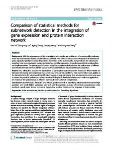
These two densities are better models than the Gaussian PDF, not only for the small amplitudes, but also for the large amplitudes where a “heavy tailed” density leads to a better fit to the observed data. Solutions to the estimation problem are given in [22] and in [13, 14, 23]. Depending on the density models, the analytic solutions can be complicated. We therefore plot the estimation characteristics in Figure 2 and 3 of these estimators and compare them to known solutions. Figure 2 plots the output of the Wiener filter, of the MMSE-LSA estimator [15], and of the esti˘ ¯ mator E S | Y using a Gaussian noise and a Laplacian speech prior [24] as a function of the input, where we assume that the input is real-valued, i.e., Yµ (k) = 0 or αµ (k) = 0. The functional relation is shown for three different a priori SNR, ηµ (k) = 15 dB, ηµ (k) = 0 dB, ηµ (k) = −10 dB. Clearly, for a fixed a priori SNR, the Wiener filter is a linear estimator, characterized by its constant slope. The MMSE-LSA estimator is close to the Wiener filter but delivers an almost constant output when the input values are much smaller than the average power which is set to two in these examples. For low SNR conditions the output of the MMSE-LSA is almost independent of the input. The estimator based on supergaussian priors, however, leads to an increased attenuation of the input when the instantaneous input value is small and a significantly larger output value when the input is large. Figure 3 plots the characteristics for the same examples as Fig. 2, however, using the “decision-directed” SNR estimation technique (6) with αη = 0.94. Now, the SNR of the preceeding signal segment is fixed. The SNR of the present segment is then a function of the instantaneous, magnitude-squared input value. In this case, all three estimators are non-linear.
2.3. MMSE Estimation Using Supergaussian Priors Although most of the known approaches use Gaussian prior densities, we may ask whether these densities are appropriate as models for the noise prior as well as for the prior density p(S ♦ ) of the speech signal. The Gaussian assumption is based on the central limit theorem [21]. However, when the DFT length is shorter than the span of correlation within the signal the asypmtotic arguments do not hold. While for many applications, the spectral components of the noise can be modeled by a Gaussian random variable, the span of correlation of voiced speech is certainly larger than the typical segment size used in mobile communications. Therefore, we must also consider supergaussian prior densities p(S ♦ ).
¯ ˘ E S | Y
4
Wiener filter MMSE−LSA Laplace speech pdf
5 4
+15 dB
3
¯ ˘ E S | Y
5
0 dB
2
−10 dB
1
2 Y
3
+15 dB
4
0 dB −10 dB
2
Sfrag replacements
0 0
Wiener filter MMSE−LSA Laplace speech pdf
3
1
(13)
1
5 PSfrag replacements
0 0 Fig. 2. Estimator characteristics for the Wiener filter (dotted), the MMSE-LSA [15] (dashed), and the MMSE estimator with a Gaussian noise and a ˘ Laplacian prior ¯ speech ˘ ¯ (solid) and three different a priori SNR. E |S|2 + E |N |2 = 2.
1
2
Y
3
4
5
Fig. 3. Estimator characteristics for the Wiener filter (dotted), the MMSE-LSA [15] (dashed), and the MMSE estimator with a Gaussian noise and a Laplacian speech prior (solid) and three different ˘ a¯priori˘SNR ¯using the “decision-directed” approach [5]. E |S|2 + E |N |2 = 2.
Good candidate densities for the DFT coefficients of speech are the Laplacian PDF, „ « 2|S ♦ | 1 exp − , (12) p(S ♦ ) = σs σs
3
1
3. BACKGROUND NOISE PSD ESTIMATION The second estimation task which arises in the processing model of Figure 1 is the estimation of the background noise power spectral density. Most of the proposals in the literature are based on
Qeq = 512 Qeq = 128
0.8 150
E{minimum}
Qeq = 64
• voice activity detection [17, 25], • soft-decision methods [26, 18],
• biased compensated tracking of spectral minima (“Minimum Statistics”) [27, 28],
Qeq = 32
0.6
Qeq = 16 0.4 Qeq = 8
or a combination thereof. In general, these methods rely on the assumptions that
0.2 Qeq = 4
Qeq = 256
• speech and noise are statistically independent,
0 0
• speech is not always present,
20
40
60
80
Qeq = 2 100 120 140
160
D
• and noise is more stationary than speech.
In what follows, we briefly outline the Minimum Statistics including the bias compensation approach.
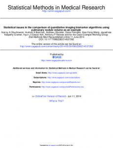
Fig. 5. Mean of minimum of D correlated short term noise power 2 = 1. estimates for σN
3.1. Minimum Statistics Noise PSD Estimation Since speech and noise are additive and statistically independent we have ˘ ¯ ˘ ¯ ˘ ¯ E |Yµ (k)|2 = E |Sµ (k)|2 + E |Nµ (k)|2 . (14)
viously, this estimate is biased towards lower values. However, the bias can be computed and compensated. It turns out, that the bias depends on the variance of the smoothed power Pµ (k) which in turn is a function of the smoothing parameter βµ (k) and the variance of the signal under consideration. For recursively smoothed power estimates and a unity noise power, Figure 5 shows the bias ˘ ¯2 as a function of D and Qeq = 2E |Nµ (k)|2 /var{Pµ (k)}. The latter is the inverse normalized variance of the smoothed power. While earlier versions of the Minimum Statistics algorithm used a fixed smoothing parameter β and hence a fixed bias compensation we note that the full potential is only developed when a time and frequency dependent smoothing method is used. This in turn requires a time and frequency dependent bias compensation [28]. The result when using the adaptive smoothing and bias compensation is shown in Figure 6 for the example of Figure 4.
Recursive smoothing of the magnitude-squared spectral coefficients leads to Pµ (k) = βµ (k) Pµ (k − r) + (1 − βµ (k)) |Yµ (k)|2
(15)
where βµ (k) is a time and frequency dependent smoothing parameter. The idea of the approach is to search for the minimum of D samples of Pµ (k − λr), λ = 0, 1, . . . , D − 1. Then, we use the minimum as first coarse estimate of the noise floor since min(Pµ (k), . . . , Pµ (k − (D − 1)r)) ˘ ¯ ˘ ¯ (16) ≈ min(E |Nµ (k)|2 , . . . , E |Nµ (k − (D − 1)r)|2 ) .
An example is shown in Figure 4 for a single frequency bin. Ob-
90
90
70 dB
80
80 |Yµ (k)|2 , (frequency bin µ = 25) smoothed power Pµ (k), (µ = 25) minimum of smoothed power
70 dB
60
60
frag replacements
PSfrag replacements
50
50
40
40
30
30
|Yµ (k)|2 , (frequency bin µ = 25) smoothed power Pµ (k), (µ = 25) minimum of smoothed power
200
400
600
segment index λ
800
200
400
600
segment index λ
800
1000
1000 Fig. 6. Magnitude-squared DFT coefficient (dotted), smoothed power, and bias corrected noise floor for the same noisy speech signal as in Figure 4.
Fig. 4. Magnitude-squared DFT coefficient (dotted), smoothed power, and noise floor for a noisy speech signal (6 dB SNR).
4
4. THE MELPe SPEECH CODER
5. MULTI-CHANNEL NOISE REDUCTION
As an application of the above techniques we consider a speech enhancement algorithm which was developed for a low bit rate speech coder. Low bit rate speech coders are especially susceptible to environmental noise as they use a parametric model to code the input signal. One such example is the Future NATO Narrowband Voice Coder which is based on the Mixed Excitation Linear Prediction (MELP) model and operates at bit rates of 1.2 and 2.4 kbps [29]. It is used for secure governmental communications and will be the successor to the well-known FS 1015 (LPC-10e) and FS 1016 (CELP) speech coding standards. The Future NATO Narrowband Voice Coder also includes an optional noise reduction preprocessor. The combined system of preprocessor and MELP coder is termed MELPe [29]. The noise reduction preprocessor [30] of the MELPe coder is based on
Further improvements are possible if we can employ more than one microphone and thus sample the sound field at more than one location. There are a number of different ways of how to exploit multiple microphone signals. The most common are • to use the spatial directivity of the microphone array;
• to adapt a single-channel post-filter based on the microphone signals. Some of these approaches are discussed, e.g., in [32]. Also we note that MAP and MMSE estimation of spectral amplitudes has been also developed for the multi-microphone case [33, 34]. 6. OUTLOOK Despite all these algorithms and many more which are not discussed here, there are still open questions which must be addressed:
• the MMSE log spectral amplitude estimator [15];
• multiplicative soft-decision gain modification [18];
• What are meaningful optimization criteria for speech enhancement and how can they be mathematically formulated?
• estimation of the a priori SNR [18];
• Which method of spectral analysis is the best or the most suitable, or, should we entirely stay in the time domain?
• adaptive gain limiting [31];
• Minimum Statistics noise power estimation [28].
• How can we improve quality without compromising intelligibility and vice versa?
The noise reduction preprocessor turns out to be very robust in a variety of noise environments and SNR conditions. Table 1 summarizes the results of a Diagnostic Acceptability Measure (DAM) test for clean and noisy conditions. As stated before, the MELP coder is highly sensitive to environmental noise. The noise reduction preprocessor helps to reduce these effects. condition no noise noisy noisy noisy
coder MELPe unprocessed MELP MELPe
DAM 68.6 45.0 38.9 50.3
• How can we combine signal theoretic and perceptual approaches? • What kind of processing approach will be optimal for signals perceived by normal hearing persons or hearing impaired persons, for signals processed by speech coders or speech recognition systems, and how are these approaches interrelated?
S. Error 0.90 1.2 1.1 0.80
• What processing takes place in the higher stages of the auditory system and how can we model it? Given all these questions it is clear that there will not be a single answer. We must, however, pay more attention to how the human mind perceives acoustic signals and processes auditory information.
Table 1. DAM scores and standard error without environmental noise and with vehicular noise (average SNR ≈ 6 dB).
7. REFERENCES
Table 2 shows results of an Diagnostic Rhyme Test (DRT) intelligibility evaluation for the same conditions as in the DAM test. We note, that the noisy but unprocessed signal has the highest intelligibility of the noisy conditions in Table 2. In conjunction with the MELP coder, the enhancement preprocessor leads to a significant improvement in terms of intelligibility. Thus, for a low bit rate speech coder, single channel noise reduction systems can improve the quality as well as the intelligibility of the coded speech. condition no noise noisy noisy noisy
coder MELPe unprocessed MELP MELPe
DRT 93.9 91.1 67.3 72.5
[1] S. Boll, “Suppression of Acoustic Noise in Speech Using Spectral Subtraction,” IEEE Trans. Acoustics, Speech and Signal Processing, vol. 27, pp. 113–120, 1979. [2] M. Berouti, R. Schwartz, and J. Makhoul, “Enhancement of Speech Corrupted by Acoustic Noise,” in Proc. IEEE Intl. Conf. Acoustics, Speech, Signal Processing (ICASSP), pp. 208–211, 1979. [3] J. Collura, “Speech Enhancement and Coding in Harsh Acoustic Noise Environments,” in IEEE Workshop on Speech Coding, pp. 162–164, 1999.
S. Error 0.53 0.37 0.8 0.58
[4] T. G¨ulzow and A. Engelsberg, “Comparison of a Discrete Wavelet Transformation and a Nonuniform Polyphase Filterbank Applied to Spectral Subtraction Speech Enhancement,” Signal Processing, Elsevier, vol. 64, no. 1, pp. 5–19, 1998. [5] Y. Ephraim and D. Malah, “Speech Enhancement Using a Minimum Mean-Square Error Short-Time Spectral Amplitude Estimator,” IEEE Trans. Acoustics, Speech and Signal Processing, vol. 32, pp. 1109–1121, December 1984.
Table 2. DRT scores and standard error without environmental noise and with vehicular noise (average SNR ≈ 6 dB).
5
[6] O. Capp´e, “Elimination of the Musical Noise Phenomenon with the Ephraim and Malah Noise Suppressor,” IEEE Trans. Speech and Audio Processing, vol. 2, pp. 345–349, April 1994.
[20] T. Lotter and P. Vary, “Noise Reduction by Maximum A Posteriori Spectral Amplitude Estimation with Supergaussian Speech Modeling,” in Proc. Intl. Workshop Acoustic Echo and Noise Control (IWAENC), 2003.
[7] P. Scalart and J. Vieira Filho, “Speech Enhancement Based on a Priori Signal to Noise Estimation,” in Proc. IEEE Intl. Conf. Acoustics, Speech, Signal Processing (ICASSP), pp. 629–632, 1996.
[21] D. Brillinger, Time Series: Data Analysis and Theory. Holden-Day, 1981. [22] J. Porter and S. Boll, “Optimal Estimators for Spectral Restoration of Noisy Speech,” in Proc. IEEE Intl. Conf. Acoustics, Speech, Signal Processing (ICASSP), pp. 18A.2.1–18A.2.4, 1984.
[8] K. Linhard and T. Haulick, “Noise Subtraction with Parametric Recursive Gain Curves,” in Proc. Euro. Conf. Speech Communication and Technology (EUROSPEECH), vol. 6, pp. 2611–2614, 1999.
[23] R. Martin, “Speech Enhancement based on Minimum Mean Square Error Estimation and Supergaussian Priors,” IEEE Trans. Speech and Audio Processing, 2003 (accepted).
[9] C. Beaugeant and P. Scalart, “Speech Enhancement Using a Minimum Least Square Amplitude Estimator,” in Proc. Intl. Workshop Acoustic Echo and Noise Control (IWAENC), pp. 191–194, 2001.
[24] R. Martin and C. Breithaupt, “Speech Enhancement in the DFT Domain Using Laplacian Speech Priors,” in Proc. Intl. Workshop Acoustic Echo and Noise Control (IWAENC), 2003.
[10] I. Cohen and B. Berdugo, “Speech Enhancement for nonstationary noise environments,” Signal Processing, Elsevier, vol. 81, pp. 2403–2418, 2001.
[25] D. Van Compernolle, “Noise adaptation in a hidden markov model speech recognition system,” Computer Speech and Language, vol. 3, pp. 151–167, 1989.
[11] D. Tsoukalas, M. Paraskevas, and J. Mourjopoulos, “Speech Enhancement using Psychoacoustic Criteria,” in Proc. IEEE Intl. Conf. Acoustics, Speech, Signal Processing (ICASSP), pp. 359–362, April 1993.
[26] J. Sohn and W. Sung, “A Voice Activity Detector Employing Soft Decision Based Noise Spectrum Adaptation,” in Proc. IEEE Intl. Conf. Acoustics, Speech, Signal Processing (ICASSP), vol. 1, pp. 365–368, 1998.
[12] S. Gustafsson, P. Jax, and P. Vary, “A Novel Psychoacoustically Motivated Audio Enhancement Algorithm Preserving Background Noise Characteristics,” in Proc. IEEE Intl. Conf. Acoustics, Speech, Signal Processing (ICASSP), pp. 397– 400, 1998.
[27] R. Martin, “Spectral Subtraction Based on Minimum Statistics,” in Proc. Euro. Signal Processing Conf. (EUSIPCO), pp. 1182–1185, 1994.
[13] R. Martin, “Speech Enhancement Using MMSE Short Time Spectral Estimation with Gamma Distributed Speech Priors,” in Proc. IEEE Intl. Conf. Acoustics, Speech, Signal Processing (ICASSP), vol. I, pp. 253–256, 2002.
[28] R. Martin, “Noise Power Spectral Density Estimation Based on Optimal Smoothing and Minimum Statistics,” IEEE Trans. Speech and Audio Processing, vol. 9, pp. 504–512, July 2001.
[14] C. Breithaupt and R. Martin, “MMSE Estimation of Magnitude-Squared DFT Coefficients with Supergaussian Priors,” in Proc. IEEE Intl. Conf. Acoustics, Speech, Signal Processing (ICASSP), 2003.
[29] T. Wang, K. Koishida, V. Cuperman, A. Gersho, and J. Collura, “A 1200/2400 BPS Coding Suite Based on MELP,” in IEEE Workshop on Speech Coding, pp. 90–92, 2002. [30] R. Martin, D. Malah, R. Cox, and A. Accardi, “A Noise Reduction Preprocessor for Mobile Voice Communication,” to be submitted, 2003.
[15] Y. Ephraim and D. Malah, “Speech Enhancement Using a Minimum Mean-Square Error Log-Spectral Amplitude Estimator,” IEEE Trans. Acoustics, Speech and Signal Processing, vol. 33, pp. 443–445, April 1985.
[31] R. Martin and R. Cox, “New Speech Enhancement Techniques for Low Bit Rate Speech Coding,” in Proc. IEEE Workshop on Speech Coding, pp. 165–167, 1999.
[16] A. Accardi and R. Cox, “A Modular Approach to Speech Enhancement with an Application to Speech Coding,” in Proc. IEEE Intl. Conf. Acoustics, Speech, Signal Processing (ICASSP), vol. 1, pp. 201–204, Mar 1999.
[32] M. Brandstein and D. Ward, eds., Microphone Arrays. Springer-Verlag, 2001. [33] R. Balan and J. Rosca, “Microphone Array Speech Enhancement by Bayesian Estimation of Spectral Amplitude and Phase,” in Proc. IEEE Sensor Array and Multichannel Signal Processing Workshop, 2002.
[17] R. McAulay and M. Malpass, “Speech Enhancement Using a Soft-Decision Noise Suppression Filter,” IEEE Trans. Acoustics, Speech and Signal Processing, vol. 28, pp. 137–145, December 1980.
[34] T. Lotter, C. Benien, and P. Vary, “Multichannel Speech Enhancement using Bayesian Spectral Amplitude Estimation,” in Proc. IEEE Intl. Conf. Acoustics, Speech, Signal Processing (ICASSP), 2003.
[18] D. Malah, R. Cox, and A. Accardi, “Tracking SpeechPresence Uncertainty to Improve Speech Enhancement in Non-Stationary Noise Environments,” in Proc. IEEE Intl. Conf. Acoustics, Speech, Signal Processing (ICASSP), pp. 789–792, 1999. [19] P. Wolfe and S. Godsill, “Simple Alternatives to the Ephraim and Malah Suppression Rule for Speech Enhancement,” in Proc. 11th IEEE Workshop on Statistical Signal Processing, vol. II, pp. 496–499, 2001.
6