Maximum Likelihood, Least Squares, statistical inference, distance mapping ... lens - CCD camera systems; ii) build, starting from this novel statistical model, ...
Statistical modeling and calibration of triangulation Lidars Anas Alhashimi1 , Damiano Varagnolo1 and Thomas Gustafsson1 1
Control Engineering Group, Department of Computer Science, Electrical and Space Engineering, Luleå University of Technology, Luleå 97187, Sweden {anas.alhashimi, damiano.varagnolo, thomas.gustafsson}@ltu.se
Keywords: Maximum Likelihood, Least Squares, statistical inference, distance mapping sensors, Lidar, nonlinear system, AIC Abstract: We aim at developing statistical tools that improve the accuracy and precision of the measurements returned by triangulation Light Detection and Rangings (Lidars). To this aim we: i) propose and validate a novel model that describes the statistics of the measurements of these Lidars, and that is built starting from mechanical considerations on the geometry and properties of their pinhole lens - CCD camera systems; ii) build, starting from this novel statistical model, a Maximum Likelihood (ML) / Akaike Information Criterion (AIC) - based sensor calibration algorithm that exploits training information collected in a controlled environment; iii) develop ML and Least Squares (LS) strategies that use the calibration results to statistically process the raw sensor measurements in non controlled environments. The overall technique allowed us to obtain empirical improvements of the normalized Mean Squared Error (MSE) from 0.0789 to 0.0046.
1
Introduction
Lidars are ubiquitously used for mapping purposes. Different types of Lidar technologies, such as Time of Flight (ToF) and triangulation, have different statistical performance. For example, ToF Lidars have generically lower bias and measurement noise variances than triangulation ones. At the same time, triangulation Lidars are generally cheaper than ToF ones. The market pull is then to increase the performance of cheaper Lidars in a cost-effective way. Improving the accuracy and precision of sensors can then be done in different ways, e.g., by improving their mechanical properties. In this paper we have a precise target: improve the performance indexes of triangulation Lidars by removing their biases and artifacts through opportune statistical manipulations of the raw information coming from the sensor. The following literature review analyzes a set of algorithms that are related to our aim. Literature review It is convenient to categorize the algorithms in the existing and relevant literature as:
• procedures for the characterization or calibration of the devices. Here characterization means a thorough quantification of the measurement noisiness of the device, while calibration means an algorithm that aims at diminishing this noisiness level; • when dealing with calibration issues, procedures for the intrinsic or extrinsic calibration. Here intrinsic means that the focus is on estimating the parameters of the Lidar itself, while extrinsic means that the focus is on estimating the parameters resulted from sensor positioning and installation. Characterization issues: several papers discuss Lidar characterization issues for both ToF [Kneip et al., 2009, Reina and Gonzales, 1997, Lee and Ehsani, 2008, Sanz-Cortiella et al., 2011, Tang et al., 2009, Tuley et al., 2005, Ye and Borenstein, 2002, Anderson et al., 2005, Alhashimi et al., 2015] and triangulation Lidars [Lima et al., 2015, Campos et al., 2016]. Notice that, at the best of our knowledge, for triangulation Lidars there exist only two manuscripts: [Lima et al., 2015],
that discusses the nonlinearity of Neato Lidars, and [Campos et al., 2016], that analyzes the effect of the color of the target on the measured distance. Importantly, [Lima et al., 2015] models nonlinear effects on the measurements and the variance of additive measurement noises as two independent effects that can be modeled with a second order polynomials on the actual distance. From statistical perspectives, thus, authors decouple the learning process into two separate parts. Calibration issues: as for the calibration issues there is a relatively large number of papers describing how to calibrate extrinsic parameters either using additional sensors (such as cameras) [Zhang and Pless, 2004b, Mei and Rives, 2006, Jokinen, 1999, Tiddeman et al., 1998], or just requiring knowledge on the motion of the Lidar itself [Andreasson et al., 2005, Wei and Hirzinger, 1998, McIvor, 1999, Zhang and Pless, 2004a]. Still considering calibration issues, there has been also a big effort on how to perform intrinsic calibration for multi-beam Lidar systems, where the results from one beam is used to calibrate the intrinsic parameters of other beams [Chen and Chien, 2012, Muhammad and Lacroix, 2010, Atanacio-Jiménez et al., 2011, Glennie and Lichti, 2010, Glennie and Lichti, 2011, Glennie, 2012, Gordon and Meidow, 2013, Mirzaei et al., 2012, Gong et al., 2013, Park et al., 2014]. As for single-beam Lidar systems, instead, [Mirzaei et al., 2012] proposes a method for the intrinsic calibration of a revolving-head 3D Lidar and the extrinsic calibration of the parameters with respect to a camera. The technique involves an analytical method for computing an initial estimate for both the Lidar’s intrinsic parameters and the Lidar-camera transformation, that is then used to initialize an iterative nonlinear least-squares refinement of all of the calibration parameters. We also mention the topic of online calibration of sensor parameters for mobile robots when doing Simultaneous localization and mapping (SLAM), very useful in navigation tasks. In this category, [Kümmerle et al., 2011] proposes an approach to simultaneously estimate a map of the environment, the position of the on-board sensors of the robot, and its kinematic parameters. These parameters are subject to variations due
to wear of the devices or mechanical effects like loading. An other similar methodology for the intrinsic calibration of depth sensor during SLAM is presented in [Teichman et al., 2013]. Statement of Contributions We focus specifically on triangulation Lidars for robotic applications, and aim to increase their performance of in a cost-effective way through statistical processing techniques. Our long term vision is to arrive at a online automatic calibration procedure for triangulation Lidars like in [Kümmerle et al., 2011, Teichman et al., 2013]; before reaching this above long-term goal, we must nonetheless solve satisfactorily the problem of calibrating triangulation Lidars offline. In this paper we thus: • propose and assess a model for the measurement process of triangulation Lidars (see Section 3 and model (1)). Our model not only generalizes the model proposed in [Lima et al., 2015, Campos et al., 2016], but also motivates it starting from mechanical and physical interpretations; • on top of this model, propose and assess a ML calibration procedure that uses data from a Motion Capture (MoCap) system. Importantly, our calibration procedure extends the one proposed in [Lima et al., 2015]: there authors decoupled the learning process into two separate stages (corresponding to estimate two different sets of parameters), while here the calibration is performed simultaneously on both the sets of parameters; • propose and assess novel ML and LS strategies for correcting the measurements from the sensor with the model inferred during the calibration stage. As reported in (31) and (32), the overall strategy is then shown to be capable to improve the normalized MSE of the raw information from the sensor from 0.0789 to 0.0046.
1.1
Organization of the Manuscript
Section 2 describes the working principles of triangulation Lidars. Based on these working principles, Section 3 proposes a statistical model of the measurement process of the device. Section 4 then validates this statistical model using data acquired through a MoCap system. Section 5 then
presents a calibration algorithm for sensors deployed in a test environment. Section 7 eventually concludes the paper with the description of future research issues.
The Triangulation Lidar Range Sensor
We now describe the functioning principle of the triangulation scanners; this discussion will be useful for explaining why the moments of the measurement noise depend on the actual measured distance. More details about the constructive details of triangulation Lidars can be found in [Blais, 2004, Konolige et al., 2008]. A prototypical triangulation Lidar is the one in Figure 1. Its working principles are then explained with the diagram in Figure 2 and its caption.
Figure 1: Photo of a triangulation Lidar.
This simple working principle helps keeping the cost of the sensor low1 , and making it commercially usable in low-cost devices like robotic vacuum cleaners. The low cost of the sensor comes nonetheless with some well-defined mechanical problems [Konolige et al., 2008]: • low-cost lens, that generate nonlinear distortion effects; • imprecise pointing accuracies, that are known of at best 6 degrees; • not rigid physical linkages among lens elements, camera, laser, and laser optics, that may suffer of distortion effects during the life of the device. 1 Incidentally, the sensor was costing $135.00 as of February 2016 in Ebay. Nonetheless, the original industrial goal was to reach an end user price of $30.00.
las e
rb
b
eam object
dk
d0
b0k
pinhole lens pinhole camera
the paral las lel o er be f am
Figure 2: Diagram exemplifying the working principle of a triangulation Lidar . The laser emits an infrared laser signal that is then reflected by the object to be detected. The beam passes through a pinhole lens and hits a CCD camera sensor. By construction, thus, the triangles defined by (b, dk ) and by (b0k , d0 ) are similar: this means that the distance to the object is nonlinearly proportional to the angle of the reflected light, and as soon as the camera measures the distance b0k one can estimate the actual distance dk using triangles similarities concepts.
As it can be seen in Figure 3, all these problems induce measurement errors; more precisely, triangulation Lidars suffer of strong nonlinearities in both the bias and the standard deviation of the measurement noise. This pushes towards finding some signal processing tools that can alleviate these problems, and keep the sensor cheap while improving its performance.
meaurements error [m]
2
laser
1 0.75 0.5 0.25 0 1
2
3
4
actual distance [m] Figure 3: Dataset
3
A novel statistical model for the Lidar measurements
Let yk be the k-th measurement returned by the Lidar when the true distance is dk . Physically, yk is computed by the logic of the sensor through a static transformation of b0k in Figure 2; we assume here that this static transformation is unknown, that b0k is not available, and that we want to improve the estimation for dk from just yk . Our ansatz for the whole transformation from dk to yk is then yk = f (dk ) + f (dk )2 ek
(1)
where • f (·) is an unknown non-linear function; � • ek ∼ N 0, σe2 is a Gaussian and white additive measurement noise. In the following Section 3.1 we motivate the presence of f (·) from mechanical considerations, while in the following Section 3.2 we motivate the presence of the f (·)2 multiplying the noise ek starting from physical considerations.
3.1
Explaining the presence of the nonlinear term f (·) in model (1)
The nonlinear term f (·) in (1) is related to what is called the radial distortion in camera calibration literature [Zhang, 2000, Weng et al., 1992, Brown, 1964, Duane, 1971]. Indeed camera lenses are notoriously nonlinear at their borders, with this nonlinearity increasing as the light beam passes closer to the lens edges. In our settings this thus happens when targets are very close or very far. Radial distortions are usually modeled in the camera calibration literature as a series of odd powers, i.e., as f (dk ) =
n X
αi d2i+1 k
(2)
i=0
where the αi ’s are the model parameters. As numerically shown during the validation of (1) in Section 4, model (2) does not describe well the evidence collected in our experiments. Indeed the specific case of triangulation Lidars lacks of the symmetries encountered in computer vision settings (see (4) and the discussion on that identity), and thus in our settings there is no need
for odd symmetries in the model (in other words, doubling d does not lead to doubling b0 ). We thus propose to remove this constraint and use a potentially non-symmetric polynomial, i.e., f (dk ) =
n X
αi dik .
(3)
i=0
The numerical validations of model (3) shown in Section 4 confirm then our physical intuition.
3.2
Explaining the presence of the multiplicative term f (dk )2 in model (1)
Assume for now that there are no lens-distortion effects. The similarity between the triangles in Figure 2 then implies dk d0 = 0. b bk
(4)
In (4) dk and b0k are generally time-varying quantities, while b and d0 are constants from the geometry of the Lidar. Assume now that the quantity measured by the CCD at time k is corrupted by a Gaussian noise, so that zk = b0k + wk with � 2 2 wk ∼ N 0, σCCD and σCCD constant �and inde2 pendent of dk . Thus zk ∼ N b0k , σCCD ; since yk =
bd0 , zk
(5)
assuming a Gaussian measurement noise on the CCD implies that yk is a reciprocal Gaussian r.v. This kind of variables are notoriously difficult to be treated (e.g., their statistical moments cannot be derive from closed form expressions starting from the original Gaussian variables). For this reason we perform a first order Taylor approximation of the nonlinear map (5) above. In general, if � � zk ∼ N b, σ 2 (6) yk = φ (zk ) then the first order Taylor approximation of the distribution of yk is [Gustafsson, 2010, (A.16)] � yk ∼ N φ(b), φ0 (b)2 σ 2 (7) where φ0 (·) is the first derivative of φ(·) w.r.t. zk . Substituting the values of our specific problem into formula (7) leads then to the novel approximated model ! � �2 bd0 −bd0 2 yk ∼ N , σCCD , (8) b0k b02 k
or, equivalently, yk = d k +
d2k ek
ek ∼ N
0, σe2
�
(9)
σ2 2 is a scaled version of σCCD where = CCD b2 d02 independent of dk and to be estimated from the data. Consider now that actually there are some lens distortion effects that imply the presence of the nonlinear term f (dk ). We can then repeat the very same discussion above, and obtain model (1) by substituting dk with f (dk ) in (9). σe2
4
Validation of the approximation (8)
The approximation introduced by the first order Taylor expansion in (8) can be seen as arbitrary. Nonetheless we show in this section that on the collected datasets it actually corresponds to the most powerful approximation in a statistical sense. To this aim we perform this two-step validation: 1. (check if the noises are independent and identically distributed (iid) and normal) perform a normality test on the yk ’s assuming that measurements are collected at a fixed distance (i.e., dk is constant): indeed ek is approximately Gaussian as much as yk is; 2. (check the order of the term multiplying ek ) compare the following alternative statistical models for the measurements yk : H0 H1 H2 H3
: : : :
yk yk yk yk
= f (dk ) + ek = f (dk ) + f (dk )ek = f (dk ) + f (dk )2 ek = f (dk ) + f (dk )3 ek
distance (i.e., dk is constant), we can perform a simple algebraic manipulation of (1) to obtain yk − yk−1 = ek − ek−1 f (dk )?
(11)
where ? indicates the order of the model (that means ? ∈ {0, . . . , 3}). (11) in its turn indicates that, since ek and ek−1 are assumed iid, � yk − yk−1 ∼ N 0, 2σe2 , ? f (dk )
? ∈ {0, . . . , 3} . (12)
Assume now that the dataset is composed by different batches each corresponding to dk ’s that are constant in the batch, but different among batches. Moreover assume that each batch is sufficiently rich to make it is possible to estimate with good confidence the unknown f (dk ) through the empirical mean of the yk relative to that batch. By combining the information from different batches it is then possible to check which model ? describes better the measured information. Indicate then with B the number of batches in the dataset, with b = 1, . . . , B the index of each batch, and with Bb the set of k’s that are relative to that specific batch b. In formulas, we thus: 1. estimate, for each model batch b = 1, . . . , B, the distance 1 X fbb = yk ; (13) |Bb | k∈Bb
2. estimate, for each model ? = 0, . . . , 3, the variance of ek as !2 B X X 1 1 y − y k k−1 c2 := . σ e b? B 2|Bb | f b b=1 k,k−1∈Bb
(10)
and check which one describes better the collected information. As for point 1 we can use standard iid tests (like the Wald-Wolfowitz runs [Croarkin and Tobias, 2006]) and standard normality tests (like the Shapiro-Wilk normality test). These tests performed on our registered data showed p-values of 0.56 and 0.42, so we can safely consider the measurement noises to be iid and Gaussian. As for point 2, we instead consider the following strategy: for every model above, assuming that measurements are collected at a fixed
(14) 3. compute, for each model ? = 0, . . . , 3, the loglikelihood of the data as h i c2 = − log P y ; d, σ e � �2 b B B b � � X X yk − fb 2? c 2 |Bb | log fbb σ e + c2 fbb2? σ e b=1 k=1 where y := [d1 , . . . , dN ]T .
[y1 , . . . , yN ]T
and d
(15) :=
In Figure 4 we then show the log-likelihoods for the different models. As it can be seen, hypothesis H 2 is the one that best describes the collected evidence.
6 H0
H1
H2
H3
Figure 4: Evaluation of (15) on the collected datasets.
A non rigorous (but graphical and intuitive) argument supporting H 2 as the hypothesis best describing the evidence is then the one offered in Figure 5. The argument goes as follows: for the exact ? ∈ {0, . . . , 3} the quantities yk − yk−1 ? ∈ {0, . . . , 3} . (16) f (dk )? should be iid independently of dk . This iid-ness is indeed a necessary condition for iid-ness of the measurement noises (one of our assumptions). Since f (·) is actually unknown, this iid-ness test must be performed by means of some estimate of f (·). In the following we use the estimator defined in Section 5 over an experiment where we manually increase the true distance dk . As it can be seen, the hypothesis H 2 is the unique yk − yk−1 one for which the quantities are hofb(dk )? moscedastic. Thus the normalizing factor ? = 2 is the unique one guaranteeing iid-ness for the measurement noises. Notice that this argument is a non rigorous wishful thinking, since we use some estimates as the ground truth; nonetheless the heteroscedasticity of the noises for ? = 0, 1, 3 indicates that these hypotheses are non-descriptive.
5
Calibrating the Lidar
Our overall goal is not just to propose the statistical model (1) describing the measurement process of the Lidar but also to find a calibration procedure for estimating the unknowns f (·) and σe2 from some collected information. Once again the long term goal is to calibrate (1) on-line and continuously using information from other sensors like odometry, ultrasonic sensors, etc. Instrumental to this future direction we now solve the first step, that is to estimate f (·) and σe2 from a dataset D = {yk , dk } in which we know dk (e.g., thanks to a MoCap system). Given our Fisherian setting, we seek for the ML estimate for both f (·) and σe2 , where we recall
yk − yk−1 fb(dk )2
7
yk − yk−1 fb(dk )
yk − yk−1
·104
yk − yk−1 fb(dk )3
i h c2 P y ; d, σ ?
8
2
3
4
distance [m] yk − yk−1 for ? = fb(dk )? 0, . . . , 3 and for increasing dk and for fb(·) computed as in Section 5. The results graphically suggest that fb(dk )2 is the unique normalizing factor for which we obtain homoscedastic samples. Figure 5: Plots of the quantities
that (due to the radial distortion hypothesis as the source of f (·), see Section 3.1) f (·) is modeled as polynomial, i.e., as f (dk ) = Pna non-symmetric i α d as in (3). Since now model (1) implies i k i=0 � yk − f (dk ) ∼ N 0, f (dk )4 σe2 , (17) it follows immediately that the corresponding negative log-likelihood is proportional to �T � L := log (det Σ) + y − f (d) Σ−1 y − f (d) (18) where • y := [y1 , . . . , yN ]T ; • d := [d1 , . . . , dN ]T ; • f (d) := [f (d1 ), . . . , f (dN )]; � • Σ := diag f (d1 )4 σe2 , . . . , f (dN )4 σe2 . Finding the ML estimates in our settings thus means: 1. solving arg min L (θ) (19) θ∈Θ
for several different n, with � � θ := α0 , . . . , αn , σe2
(20)
and Θ the set of θ ∈ Rn+1 for which σe2 > 0; 2. deciding which n is the best one using some model order selection criterion, e.g., AIC. Unfortunately problem (19) is not convex, so it neither admits a closed form solution nor it can be easily computed using numerical procedures. Solving problem (19) is thus numerically difficult. Keeping in mind that our long-term goal is the development of on-line calibration procedures, where numerical problems will be even more complex, we strive for some alternative calibration procedure.
5.1
An approximate calibration procedure
We here propose an alternative estimator that trades off statistical performance for solvability in a closed form. We indeed propose to seek an estimate for θ in (20) by using the alternative model yk = f (dk ) + d2k ek , (21) that differs from (1) only for the fact that the noise is multiplied by d2k instead of f (dk )2 . This approximation is intuitively meaningful, since f (dk ) represents a distortion term induced by the pinhole lens: ideally, indeed, f (dk ) should be equal to dk . Assuming model (21) it is now possible do derive a ML estimator of θ. Indeed dividing both sides of (21) by d2k we get yk = g(dk ) + ek d2k
(22)
with y 1
−2 d1 .. H := . d−2 N
g(dk ) =
n X
αi di−2 k .
5.2
This means that the estimation problem can be cast as the problem of estimating the parameters T α := [α0 , . . . , αn ] and the noise variance σe2 describing the linear system α0 � � yk −2 n−2 . = d . . . d (24) .. + ek , k k d2k αn
5.2.1
(25)
···
dn−2 N
(26)
Using the calibration results to estimate dk
Computing the ML estimate of dk
Rewriting model (3) as
f (dk ) = dTk α
d0k d1k dk := . ..
(27)
dnk
and equating the score of yk parametrized by α and σe2 to zero leads to the equation � � yk − dk α yk − dk (I − K) α = σe2 d4k (28) � � 1 n K := diag 0, , . . . , . 2 2
(29)
b and This means that estimating dk from yk , α c2 can be performed by solving (28) in dk after σ e substituting the real values α and σe2 with their estimates. Since polynomial (28) is quartic for n = 0, 1, 2, and of order at least 6 for any other n, the ML estimate for dk must then either rely on complex algebraic formulas or numerical roots finding methods. 5.2.2
for which the ML solution is directly �−1 T b = HT H α H ye 1 c2 = b T (e b (e y − H α) y − H α) σ e N
.. .
d21 . ye := .. . yN d2N
b and Once the sensor has been calibrated, i.e., a α c2 have been computed, it is possible to invert σ e the process and use the learned information for testing purposes. This means that given some measurements yk collected in an unknown envic2 , estimate dk . b and σ ronment we can, through α e
(23)
i=0
Notice that the procedure above does not determine the model complexity n. For inferring this parameter we then propose to rely on classical model order selection criteria such as AIC.
with
where (cf. (3))
···
dn−2 1
Computing the LS estimate of dk
Given our assumption (3) on the structure of f (·), and given an estimate fb for f , the problem of estimating dk from yk is the one of minimizing
Thus if the Lidar has heavy nonlinear radial distortions (that means that it requires high order polynomials f (·)) then one is again required to compute polynomials’ roots. Notice also that some of the roots above may not belong to the measurement range of the sensor (e.g., some roots may be negative); these ones can safely be discarded from the set of plausible solutions. The other ones, instead, are equally plausible. This raises a question on how to decide which root should be selected among the equally plausible ones. This question is actually non-trivial, and cannot be solved by means of the frequentist approach used in this manuscript. We thus leave this question unanswered for now, and leave it as a future research question, that will probably be solved by using Bayesian formalisms.
polynomial order 1 2 3 4
AIC score -5.774 -7.380 -5.824 -3.890
Table 1: AIC scores for the different models complexities involved in the training set of Figure 7.
selection, we empirically detected that n = 2 was always the best choice when using AIC measures. E.g., for the dataset shown in Figure 7 we obtained the AIC scores reported in Table 1. measurement error [m]
�2 the squared loss yk − fb(dk ) . Once again, the problem is of finding the roots of a polynomial, since the solutions of the LS problem above are directly n � � o dbk ∈ de s.t. yk − fb de = 0 . (30)
1 training set order 1 order 2 order 3
0.75 0.5 0.25 0 0
1
2
3
4
5
actual distance [m]
6
Numerical experiments
Our experiments consist in a robot with the Lidar mounted on top moving with piecewise constant speeds towards a target. We recorded several datasets for training and testing purposes, consisting of the Lidar measurements and a ground truth information collected by a MoCap system (see Figure 6). Training datasets were
Figure 7: A typical training set collected in our experiments. The plotted quantities correspond to the measurement errors and to the polynomial models fitting these errors.
The estimated α and σe2 were also used for testing purposes to refine the estimate of the distances dk in non-controlled environments. Notice that the selected model order was always 2, so it was always possible to solve the LS problem in a closed form and also discard one of the roots in (30), so that the set of roots was always a singleton. As shown in Figure 8, dbk is much closer to dk than yk . For example, the empirical normalized MSEs for the test set in Figure 8 were
2 bk − dk N d
X 1 = 0.0046, (31) 2 N kdk k k=1 N 2 1 X kyk − dk k = 0.0789. 2 N kdk k k=1
Figure 6: Experimental setup used for recording the dataset. The Lidar was mounted over a Pioneer 3AT robot facing an obstacle; the photo moreover shows some of the cameras of the MoCap system.
thus initially used to estimate α and σe2 as described in Equation (25). As for the model order
7
(32)
Conclusions
We derived, starting from a combination of physical and statistical considerations, a model
measured distance [m]
6
test set MoCap estimated
5 4 3 2 1 0
0
1
2
3
4
5
6
actual distance [m] Figure 8: Effects of the estimation procedure on the original Lidar measurement. It can be noticed how the overall strategy removes the nonlinearities induced by the pinhole lens - CCD camera system.
that describes the statistical behavior of the measurements returned by triangulation Lidars. This statistical model, given in (1), is based on two assumptions: 1. the effects of radial distortions in the pinhole lens can be captured by means of a polynomial function; 2. the nonlinearities induced by the geometry of the laser-CCD system can be captured by means of a heteroscedastic noise which standard deviation depends in first approximation quadratically with the measured distance. This model, validated through some experiments on real devices, allows to build tailored triangulation Lidars calibration strategies that follow the classical training-testing paradigm: • in the training phase, collect information in a controlled environment and use it to estimate through ML paradigms the parameters defining the statistical behavior of the sensor; • in the test phase, use this information and some statistical inference techniques such as ML or LS to correct the measurements from the sensor when this is in a non-controlled environment. It turns then out that both the ML and LS estimation strategies may be numerically demanding, specially for sensors suffering of strong radial distortions in the pinhole camera. In this case, indeed, the estimators may require to use numerical root finding procedures and lead to some computational disadvantages.
Irrespectively of these issues, that can in any case be mitigated by limiting the complexity of the polynomials describing the radial distortions, the estimation strategies above have been proved to be effective in our tests. Real-life experiments indeed showed that the techniques allow to reduce the empirical MSE of the sensor of a factor 17.15. Despite this promising result, the research associated to triangulation Lidars is not finished: indeed, by following a classical training-testing approach, the techniques above present some limitations. Different sensors may in fact differ even if nominally being constructed in the same way. Moreover sensors may change their statistical behavior in time, due to aging or mechanical shocks. This means that techniques based on results from a controlled environment on just one sensor and just once are eventually not entirely meaningful. A robust approach must indeed perform continuous learning for each sensor independently in a non-controlled environment by performing information fusion steps, e.g., combining also information from other sensors like odometry, ultrasonic and accelerometers. This information-fusion continuous-learning algorithm nonetheless must be based on some preliminary results on what are the statistical models of triangulation Lidars and on how inference can be performed on them. This paper can thus be seen as the first step towards more evolved strategies.
REFERENCES [Alhashimi et al., 2015] Alhashimi, A., Varagnolo, D., and Gustafsson, T. (2015). Joint temperaturelasing mode compensation for time-of-flight lidar sensors. Sensors, 15(12):31205–31223. [Anderson et al., 2005] Anderson, D., Herman, H., and Kelly, A. (2005). Experimental characterization of commercial flash ladar devices. In International Conference of Sensing and Technology, volume 2. [Andreasson et al., 2005] Andreasson, H., Triebel, R., and Burgard, W. (2005). Improving plane extraction from 3d data by fusing laser data and vision. In Intelligent Robots and Systems, 2005.(IROS 2005). 2005 IEEE/RSJ International Conference on, pages 2656–2661. IEEE. [Atanacio-Jiménez et al., 2011] Atanacio-Jiménez, G., González-Barbosa, J.-J., Hurtado-Ramos, J. B., Ornelas-Rodríguez, F. J., JiménezHernández, H., García-Ramirez, T., and GonzálezBarbosa, R. (2011). Lidar velodyne hdl-64e calibration using pattern planes. International Journal of Advanced Robotic Systems, 8(5):70–82. [Blais, 2004] Blais, F. (2004). Review of 20 years of range sensor development. Journal of Electronic Imaging, 13(1). [Brown, 1964] Brown, D. C. (1964). An advanced reduction and calibration for photogrammetric cameras. Technical report, DTIC Document. [Campos et al., 2016] Campos, D., Santos, J., Gonçalves, J., and Costa, P. (2016). Modeling and simulation of a hacked neato xv-11 laser scanner. In Robot 2015: Second Iberian Robotics Conference, pages 425–436. Springer. [Chen and Chien, 2012] Chen, C.-Y. and Chien, H.J. (2012). On-site sensor recalibration of a spinning multi-beam lidar system using automaticallydetected planar targets. Sensors, 12(10):13736– 13752. [Croarkin and Tobias, 2006] Croarkin, C. and Tobias, P. (2006). Nist/sematech e-handbook of statistical methods. NIST/SEMATECH, July. Available online: http://www.itl.nist.gov/div898/handbook. [Duane, 1971] Duane, C. B. (1971). Close-range camera calibration. Photogrammetric engineering, 37(8):855–866. [Glennie, 2012] Glennie, C. (2012). Calibration and kinematic analysis of the velodyne hdl-64e s2 lidar sensor. Photogrammetric Engineering & Remote Sensing, 78(4):339–347. [Glennie and Lichti, 2010] Glennie, C. and Lichti, D. D. (2010). Static calibration and analysis of the velodyne hdl-64e s2 for high accuracy mobile scanning. Remote Sensing, 2(6):1610–1624. [Glennie and Lichti, 2011] Glennie, C. and Lichti, D. D. (2011). Temporal stability of the velodyne
hdl-64e s2 scanner for high accuracy scanning applications. Remote Sensing, 3(3):539–553. [Gong et al., 2013] Gong, X., Lin, Y., and Liu, J. (2013). 3d lidar-camera extrinsic calibration using an arbitrary trihedron. Sensors, 13(2):1902–1918. [Gordon and Meidow, 2013] Gordon, M. and Meidow, J. (2013). Calibration of a multi-beam laser system by using a tls-generated reference. ISPRS Annals of Photogrammetry, Remote Sensing and Spatial Information Sciences II-5 W, 2:85–90. [Gustafsson, 2010] Gustafsson, F. (2010). Statistical sensor fusion. Studentlitteratur,. [Jokinen, 1999] Jokinen, O. (1999). Self-calibration of a light striping system by matching multiple 3-d profile maps. In 3-D Digital Imaging and Modeling, 1999. Proceedings. Second International Conference on, pages 180–190. IEEE. [Kneip et al., 2009] Kneip, L., Tâche, F., Caprari, G., and Siegwart, R. (2009). Characterization of the compact hokuyo urg-04lx 2d laser range scanner. In Robotics and Automation, 2009. ICRA’09. IEEE International Conference on, pages 1447– 1454. IEEE. [Konolige et al., 2008] Konolige, K., Augenbraun, J., Donaldson, N., Fiebig, C., and Shah, P. (2008). A low-cost laser distance sensor. In Robotics and Automation, 2008. ICRA 2008. IEEE International Conference on, pages 3002–3008. IEEE. [Kümmerle et al., 2011] Kümmerle, R., Grisetti, G., and Burgard, W. (2011). Simultaneous calibration, localization, and mapping. In Intelligent Robots and Systems (IROS), 2011 IEEE/RSJ International Conference on, pages 3716–3721. IEEE. [Lee and Ehsani, 2008] Lee, K.-H. and Ehsani, R. (2008). Comparison of two 2d laser scanners for sensing object distances, shapes, and surface patterns. Computers and electronics in agriculture, 60(2):250–262. [Lima et al., 2015] Lima, J., Gonçalves, J., and Costa, P. J. (2015). Modeling of a low cost laser scanner sensor. In CONTROLOâĂŹ2014– Proceedings of the 11th Portuguese Conference on Automatic Control, pages 697–705. Springer. [McIvor, 1999] McIvor, A. M. (1999). Calibration of a laser stripe profiler. In 3-D Digital Imaging and Modeling, 1999. Proceedings. Second International Conference on, pages 92–98. IEEE. [Mei and Rives, 2006] Mei, C. and Rives, P. (2006). Calibration between a central catadioptric camera and a laser range finder for robotic applications. In Robotics and Automation, 2006. ICRA 2006. Proceedings 2006 IEEE International Conference on, pages 532–537. IEEE. [Mirzaei et al., 2012] Mirzaei, F. M., Kottas, D. G., and Roumeliotis, S. I. (2012). 3d lidar–camera intrinsic and extrinsic calibration: Identifiability and analytical least-squares-based initialization.
The International Journal of Robotics Research, 31(4):452–467. [Muhammad and Lacroix, 2010] Muhammad, N. and Lacroix, S. (2010). Calibration of a rotating multi-beam lidar. In Intelligent Robots and Systems (IROS), 2010 IEEE/RSJ International Conference on, pages 5648–5653. IEEE. [Park et al., 2014] Park, Y., Yun, S., Won, C. S., Cho, K., Um, K., and Sim, S. (2014). Calibration between color camera and 3d lidar instruments with a polygonal planar board. Sensors, 14(3):5333–5353. [Reina and Gonzales, 1997] Reina, A. and Gonzales, J. (1997). Characterization of a radial laser scanner for mobile robot navigation. In Intelligent Robots and Systems, 1997. IROS’97., Proceedings of the 1997 IEEE/RSJ International Conference on, volume 2, pages 579–585. IEEE. [Sanz-Cortiella et al., 2011] Sanz-Cortiella, R., Llorens-Calveras, J., Rosell-Polo, J. R., GregorioLopez, E., and Palacin-Roca, J. (2011). Characterisation of the lms200 laser beam under the influence of blockage surfaces. influence on 3d scanning of tree orchards. Sensors, 11(3):2751– 2772. [Tang et al., 2009] Tang, P., Akinci, B., and Huber, D. (2009). Quantification of edge loss of laser scanned data at spatial discontinuities. Automation in Construction, 18(8):1070–1083. [Teichman et al., 2013] Teichman, A., Miller, S., and Thrun, S. (2013). Unsupervised intrinsic calibration of depth sensors via slam. In Robotics: Science and Systems. Citeseer. [Tiddeman et al., 1998] Tiddeman, B., Duffy, N., Rabey, G., and Lokier, J. (1998). Laser-video scanner calibration without the use of a frame store. In Vision, Image and Signal Processing, IEE Proceedings-, volume 145, pages 244–248. IET. [Tuley et al., 2005] Tuley, J., Vandapel, N., and Hebert, M. (2005). Analysis and removal of artifacts in 3-d ladar data. In Robotics and Automation, 2005. ICRA 2005. Proceedings of the 2005 IEEE International Conference on, pages 2203– 2210. IEEE. [Wei and Hirzinger, 1998] Wei, G.-Q. and Hirzinger, G. (1998). Active self-calibration of hand-mounted laser range finders. Robotics and Automation, IEEE Transactions on, 14(3):493–497. [Weng et al., 1992] Weng, J., Cohen, P., and Herniou, M. (1992). Camera calibration with distortion models and accuracy evaluation. IEEE Transactions on Pattern Analysis & Machine Intelligence, 14(10):965–980. [Ye and Borenstein, 2002] Ye, C. and Borenstein, J. (2002). Characterization of a 2-d laser scanner for mobile robot obstacle negotiation. In ICRA, pages 2512–2518.
[Zhang and Pless, 2004a] Zhang, Q. and Pless, R. (2004a). Constraints for heterogeneous sensor auto-calibration. In Computer Vision and Pattern Recognition Workshop, 2004. CVPRW’04. Conference on, pages 38–38. IEEE. [Zhang and Pless, 2004b] Zhang, Q. and Pless, R. (2004b). Extrinsic calibration of a camera and laser range finder (improves camera calibration). In Intelligent Robots and Systems, 2004.(IROS 2004). Proceedings. 2004 IEEE/RSJ International Conference on, volume 3, pages 2301–2306. IEEE. [Zhang, 2000] Zhang, Z. (2000). A flexible new technique for camera calibration. Pattern Analysis and Machine Intelligence, IEEE Transactions on, 22(11):1330–1334.