PAPER Special section on Analog Circuit Techniques supporting the System LSI Era. Statistical Modeling of Device Characteristics with Systematic. Variability.
IEICE TRANS. FUNDAMENTALS, VOL.E84–A, NO.2 FEBRUARY 2001
529
PAPER
Special section on Analog Circuit Techniques supporting the System LSI Era
Statistical Modeling of Device Characteristics with Systematic Variability Kenichi OKADA† , Student Member and Hidetoshi ONODERA† , Member
SUMMARY The variabilities of device characteristics are usually regarded as a normal distribution. If we consider the variabilities over the whole wafer, however, they cannot be expressed as a normal distribution due to the existence of global systematic component. We propose a statistical model, characterizing the global systematic component according to the distance from the center of the wafer, which can express the variabilities over the whole wafer statistically. key words: MOSFET, variability, systematic, stochastic
1.
Introduction
The consideration for variabilities of device characteristics has been an important theme in designing CMOS integrated circuits. The variabilities arise from two sources of process non-uniformity: a local stochastic component and a global systematic component [1]–[3]. The former is a white noise caused by a stochastic nature of fabrication processes. It has no spatial dependence, and causes a parameter mismatch for a pair of closely-arranged transistors. The latter represents a systematic parameter-value distribution over the whole wafer which is caused by, for example, a non-uniform thermal distribution during a fabrication process or the lens aberration during a photolithographic process. It consists of very low spatial frequency, and it is regarded as a smooth variation over the wafer. It is a common practice to treat the variabilities as a normal distribution. It is true within a limited area on a wafer, such as within a chip or a small circuit. If we consider the variabilities over the whole wafer, however, it is not expressed as a normal distribution due to the existence of the systematic variability. We should therefore build a global model of the systematic variability which is valid over the whole wafer. Together with the global model, we need to consider the local stochastic variability. The characteristics of adjacent transistors differ because of the local stochastic variability. In static timing analysis, the characteristics of the transistors are usually assumed to be constant across a chip, but in fact, they are different. The existence of the local Manuscript received July 3, 2000. Manuscript revised September 13, 2000. † The authors are with Department of Communications and Computer Engineering, Kyoto University, Sakyo-ku, Kyoto, 6068501 Japan
stochastic variability has a large effect on the statistical timing behavior of a circuit, as we will explain later. It is therefore important to have a proper model for the local stochastic variability. In this paper, we propose a set of statistical models, which characterize both the local stochastic variability and the global systematic variability. We will explain a method for reproducing the device characteristics by the proposed models and show experimental results. An example of statistical analysis is also presented. This paper is organized as follows. Section 2 explains previous work. Section 3 presents a case study showing the impact of the process variability. Section 4 proposes a set of statistical models for the local and global variabilities, and explains how the process variability is reproduced from our models. Section 5 reports experimental results. Finally, Sect. 6 concludes our discussion. 2. Previous Work In this section, we briefly review statistical MOSFET models proposed so far. We then discuss a necessary condition for a statistical model. Statistical models for the local stochastic component have been proposed in [3]–[7]. Among them, Pelgrom’s model[4] is most widely accepted. He proposed a mismatch model for a transistor pair with the same size. The model characterizes all sources of mismatch as the stochastic variation of the difference in the parameter values which model a MOSFET behavior: A2 2 σ2 (∆P) = ∆P + S ∆P D2 . (1) WL The function σ(∆P) represents the standard deviation of the parameter ∆P. The parameters W and L are the gate-width and gate-length of the transistors spaced by the distance D. The parameters A∆P and S ∆P are process-dependent constants. The first term represents the local stochastic variation, and the second term represents the global systematic variation which is modeled as an additional stochastic process with a long correlation distance. The other models for the local stochastic component are proposed in [5], [7]. Bastos’ model[5] aims to represent more accurate matching property as in Eq. (2).
IEICE TRANS. FUNDAMENTALS, VOL.E84–A, NO.2 FEBRUARY 2001
530
A21∆P A22∆P A23∆P 2 + + + S ∆P D2 (2) WL WL2 W 2 L These models have additional terms considering size dependence, because the MOSFET parameter P depends on its size. However, the MOSFET parameters do not only have size dependence but also have bias dependence, so the statistical model should describe both dependences. Felt suggests that the Pelgrom’s model can not express the systematic component precisely, and he modeled the systematic variability as a linear gradient across the chip [2], [3]. The model, however, does not describe the distribution of the systematic variability. A method is reported in [8] where all the measured/extracted parameters with stochastic and systematic variations are directly used for statistical analysis instead of modeling. The method reproduces a realistic distribution, but it does not consider spatial dependence. We cannot therefore estimate a layout effect by the method. Since the method does not build a model, it cannot be applied unless we collect actual measured data from various wafers. It is important for a statistical model to consider size and bias dependences and to reproduce a realistic distribution with spatial dependence. Previous models do not satisfy all the necessary conditions explained above. σ2 (∆P) =
3.
Impact of Process Variabilities
In this section, we explain the effect of process variabilities on circuit performance. We show a case study for the impact of local stochastic variability. Also we discuss a necessity to consider the distribution of the global systematic variability. First, we explain the impact of the local stochastic variability within a chip (intra-chip variability). In conventional timing analysis, the characteristics of transistors are usually assumed to be constant within a chip, but actually characteristics of the adjacent transistors differ from each other due to local stochastic fluctuation. The fluctuation affects the statistical characteristics of the circuit delay[9]. Suppose a logic-gate that has n-input and 1-output ports. The latest signal-arrival time transitions at the output, T out is represented as follows. n
T out = max(T i + ti ), i=1
(3)
where T i is the latest arrival time of signals at the i-th input, and ti is the gate delay time from the i-th input to the output. For example, Fig. 1 shows a pyramidal circuit consisting of 15-level NAND gates. Every path from the input port to the output port may have the longest delay. Taking this circuit as an example, we show how the local stochastic fluctuation affects the delay of the critical path in a different manner than the global systematic fluctuation. We examine two cases where the first case(Case A) contains both fluctuations while the second case(Case B) contains the global
15
Fig. 1
4
3
2
1
A pyramidal circuit consisting of NAND gates.
systematic fluctuation only. In Case A, the amount of fluctuation in the delay of each inverter has a common component by the global systematic variability and an independent component by the local stochastic variability, denoted by DA g and DA l respectively. We assume that those components has the same amount of standard deviations with the mean values being zero. σ(DA g) = σ(DA l)
(4)
DA g = DA l = 0
(5)
In Case B, only the global systematic variability DB g exists with the amount being equal to the total amount of fluctuation in Case A. That is, σ2 (DB g) = σ2 (DA g) + σ2 (DA l)
(6)
DB g = DB l = 0.
(7)
Figure 2 shows the distributions of the critical path delay in both cases. The horizontal and the vertical axes represent the delay of the critical path and the population respectively. The filled bars express the distribution for Case A(local and global variability), while the open bars indicate the distribution for Case B(without local variability). It can be seen that, with the local variability, the distribution becomes narrower and the mean value becomes larger than that without the local variability . Random component in delay at each gate helps to balance the overall path-delay, which contributes to the narrowing of the distribution. Also, the max operation Eq.(3) push the mean value higher. Correct modeling of both components are crucial for accurate timing analysis. Next, we focus on the impact of the global systematic variability. If we limit our attention to the systematic variability within a chip, it can be modeled as a linear gradient across the chip. The farther the transistors are placed, the worse their characteristics differ by the systematic variability. The variation for the global systematic component on the overall wafer is known to be as large as the variation of the local stochastic component[1], [6]. Therefore, a large circuit should be simulated with its spatial information. The
OKADA and ONODERA: STATISTICAL MODELING OF DEVICE CHARACTERISTICS WITH SYSTEMATIC VARIABILITY
531
simulated with the local variability
simulated without the local variability
1.4
1.5
1.6
1.7
1.8 (ns)
Fig. 2 Distributions of the delay for the circuit in Fig. 1. The horizontal axis and the vertical axis represent the delay of the circuit and the population respectively. The filled bars are populations of delays simulated with the local stochastic variability. The open bars are populations of delays simulated without the local stochastic variability.
eter extraction. Besides the size dependency, these parameters have bias dependency. Therefore, a statistical model should have the ability for expressing both dependencies. Also, the model should characterize the behavior of MOSFET in deep-submicron processes. Here we propose a simple model according to the Pelgrom’s formula. We do not model MOSFET parameters such as VT H and β, but characterize the variability for these five physical parameters: the doping concentration NCH , the gate oxide thickness T OX , the mobility µ0 , the deviation of the gate-width ∆W and the deviation of the gate-length ∆L. These physical parameters do not have the size and bias dependences, so the parameters can be characterized by the area according to the Pelgrom’s law. The physical parameters are transformed to the MOSFET parameters considering the size and bias dependencies. Thus, the size and bias dependencies are taken into account in the target MOSFET model. Our models are expressed as follows.
systematic component can be regarded as a smooth variation over the wafer, so the global systematic variability cannot be described by a normal distribution. We show the measured distribution and impact for the circuit performance in Sect. 5.1. 4.
σ2 (T OX ) = σ2 (µ0 ) =
Characterization of Process Non-uniformities
In previous sections, we discussed the required condition for the statistical model. In this section, we propose a set of models for the local stochastic variability and the global systematic variability and explain the modeling methodology of the process variability. The statistical model must characterize the size and bias dependences and reproduce a realistic distribution with spatial dependence. Previous models lack some part of the necessary conditions. Especially, the reproduction of the systematic variability with a realistic distribution is not well studied. To reproduce the spatial dependence and the realistic distribution precisely, we propose two separate models for the local stochastic and global systematic variability. The first model characterizes the local stochastic variability according to the Pelgrom’s formula. They are explained in the following parts. The second model characterizes the global systematic variability as a function of the position of the transistor on the wafer. 4.1
σ2 (NCH ) =
Modeling of Local Stochastic Variability
Models for the local stochastic variability of MOSFET parameters such as threshold voltage VT H and transconductance factor β have been proposed in [3]–[7]. These parameters have size and bias dependencies. Some models [5], [7] have additional terms to consider the size dependence as in Eq. (2), which in term introduces some difficulties in param-
A2NCH WL A2TOX WL A2µ0
WL A2 σ2 (∆L) = ∆L2 WL A2 σ2 (∆W) = ∆W , W2L
(8) (9) (10) (11) (12)
where W and L are effective geometries which may be slightly different from the drawn extensions. There differences are important for small structures[6]. These parameters, ANCH , ATOX , Aµ0 , A∆W and A∆L , are process-dependent constants. The function σ(P) expresses the standard deviation of the difference between a physical parameter and its mean value. Our method uses the concept of an intermediate model [10] to transform the physical parameters to MOSFET parameters with the size and bias dependences. Statistical set of MOSFET parameters is generated from the statistical information of the physical parameters with the correlation of the parameters. It is important how well the physical parameters can explain its physical nature. Using the intermediate model, we can get such parameters. Parameters, spoiled by a numerical optimization during an extraction of physical parameters, are not suitable for our model, which are assumed to have artificial dependences in the size or the bias. 4.2
Modeling of Global Systematic Variability
The systematic variability is resulted from a global nonuniformity of process, so its gradient varies slowly. The
IEICE TRANS. FUNDAMENTALS, VOL.E84–A, NO.2 FEBRUARY 2001
532
global systematic variability of physical parameters over the whole wafer is assumed to be approximated with a low dimensional equation. We use Eq. (13) or (14), which are empirical equations. g(x, y) = a(x2 + y2 ) + bx + cy + d √ g(r, θ) = ar2 + b2 + c2 r cos(θ + α) + d
(13) (14)
Equation (13) uses the orthogonal coordinates (x, y) while Eq. (14) uses the polar coordinates (r, θ). The variables x and y are equivalent to r cos θ and r sin θ respectively. The origin of those coordinates is assumed to be the center of the wafer. We show an example of the approximation by Eq. (13). Figure 3 is a three dimensional plot of the systematic variation of SPICE parameter VT H0 of a PMOS. The threshold voltage of a long channel device VT H0 can well explain the doping concentration NCH . The systematic variation is calculated from the mean value of measurements within a small area in order to separate the global systematic component from the local stochastic component. Each point on the plane (a) is averaged over 10 transistors in a local area. The plane (b) represents an approximation of the plane (a) by a quadratic function. The RMS(Root Mean Square) error of the approximation is 0.4%. Next, we discuss the statistical modeling of the global systematic variability. Rearranging the parameters of Eq. (13) will lead to the following equation for the systematic variation over the whole wafer. G(r, θ) = Ar2 + Br cos(θ + α) + C,
(15)
where the parameters A, B, C and α characterize the systematic variation of a single wafer. The variation of wafers, in the same or different lot, is estimated with the statistics of the parameters(A, B, C and α). The statistics include the correlation of the parameters, so it is better to reduce the parameters in order to simplify statistical analysis and the statistical characteristic of parameters. There is an experience that the performance of circuits Vth0
(a)measured (b)approximated
-40
20 -20
(mm)
0 0
20
40 (mm)
-20
Fig. 3 Three Dimensional plot of the systematic variation(PMOS VT H0 ). Each point on the plane(a) is the average of 10 transistors in a local area. The plane(b) represents an approximation of the plane(a) by a quadratic equation.
are inferior on the edge of wafer. In other words, the larger the parameter r in Eq. (15) increases, the more the parameters of a MOSFET differ from the mean values. Based on this observation, we make an assumption that the distribution of the systematic variations are equivalent among the points which have the same distance r from the center of a wafer, which assumption is exploited for the derivation of a statistical model for the systematic variation. Suppose that consider two sets (S 1 and S 2 ) of the systematic variation on any two points (r, θ1 ) and (r, θ2 ) within a wafer. They are expressed as follows. S1 = = S2 = =
{g(r, θ1 )|0 ≤ α < 2π} {Ar2 + Br cos(θ1 + α) + C|0 ≤ α < 2π} {g(r, θ2 )|0 ≤ α < 2π} {Ar2 + Br cos(θ2 + α) + C|0 ≤ α < 2π}
(16) (17)
and 0 ≤ r ≤ R, 0 ≤ θi < 2π, θ1 , θ2 ,
(18) (19) (20)
where R is a radius of the wafer. From the assumption, S 1 should be equivalent to S 2 , which requests that the parameter α is a random number from 0 to 2π with a uniform distribution in the model. Also from the assumption, the distributions of the systematic variability does not depend on θ. Thus we obtain the following statistical model for the systematic variability with model parameters A, B and C. G(r) = Ar2 + Br cos α + C.
(21)
Our model characterizes the systematic variability according to the distance from the center of a wafer. Our model is expected to work well when the distributions of the systematic variability are equivalent among points which have the same distance from the center of a wafer. 4.3
Probability Density of Systematic Variability
Given the global variability model of Eq. (21) and its parameters (A, B and C), one of our interests is the distribution of physical parameters expressed by Eq. (21). The distribution is expressed as the probability density p(g) for the value g of the physical parameters. The probability density p(g) is calculated from the area that has the same value of g. The area with the same g is derived from Eq.(15) considering the geometry of the global variability. The radius of the wafer is represented by the parameter R. The distance from the center of the wafer(the origin of the polar coordinates) and the pole(the center) of the global variability expressed by B . Categorizing the value of R the quadratic equation is 2A B with respect to the distance 2A , and further the polarity of
OKADA and ONODERA: STATISTICAL MODELING OF DEVICE CHARACTERISTICS WITH SYSTEMATIC VARIABILITY
533
parameter A, we can derive the probability density p(g) as follows. B 0 < R < 2A : 0 (g