Statistical Models for Term Compression James Cheney Cornell University
[email protected] Abstract Symbolic tree data structures, or terms, are used in many computing systems. Although terms can be compressed by hand, using specialized algorithms, or using universal compression utilities, all of these approaches have drawbacks. We propose an approach which avoids these problems by using knowledge of term structure to obtain more accurate predictive models for term compression. We describe two models that predict child symbols based on their parents and locations. Our experiments compared these models with first-order Markov sequence models using Huffman coding and found that one model can obtain 20% better compression in similar time, and the other, simpler model can obtain similar compression 40% faster. These compression models also approach, but do not exceed, the performance of gzip.
1
Introduction
Computing systems frequently deal with symbolic tree data structures, which are also known as terms in universal algebra and logic. For example, arithmetic expressions such as 2x2 − 3x + 1 can be represented as terms. Other common term systems include machine code and compiler intermediate representations, parse trees, mathematical formulas and proofs, and structured documents in markup languages like SGML and HTML. When large terms must be stored, processed, or sent over a network, we might like to employ compression techniques to use resources as efficiently as possible. The state of the art of term compression can be divided into the following three approaches. We can develop efficient term representations and make common abbreviations by hand. We can compress certain kinds of terms using specialized algorithms, for example program code[6, 8], syntax tree[7, 10], and unlabeled tree compression[9]. Finally, we can use utilities based on universal compression algorithms to compress sequential representations of terms. Each of these approaches to term compression has a disadvantage. Compressing by hand can lead to good compression for many term languages, but is tedious and inefficient. Specialized algorithms are effective and efficient, but may apply only to particular languages. Many universal compression algorithms are fast and can be applied to any data, but are based on sequential models of information generation which do not always model terms accurately, so they may not obtain the best compression. Our goal is to develop universal, effective, and efficient term compression techniques which avoid all these problems. This paper presents an approach which uses knowledge of term structure to build accurate universal statistical models of terms, and uses these models to compress terms faster or more effectively than comparable sequential methods. First we review the well-known independent and Markov sequence generation models to which our models will be compared. We then give a working definition of term languages that is general enough for many applications. We present two statistical term models that are related to Markov random fields over trees[13, 16]. In the first model, a symbol’s value is predicted by value of its parent in the tree. The second model also uses the symbol’s argument position as a predictor. We believe that these models are general enough to apply to many different term languages and simple enough that they can be implemented efficiently. We conducted experiments using these models to perform Huffman coding and found that term models have a better time-effectiveness tradeoff than first-order Markov sequence models. The first term model obtains similar compression faster, and the second obtains better compression in 1
comparable time. In further experiments, we compared the term models with gzip and found that our best model compresses nearly as well, and it seems likely that with slight changes we could obtain better compression. Finally, we discuss related research and prospects for further work on term compression.
2
Background: Sequential Models
We will begin by describing two simple statistical models of sequences: an independent model and a first-order Markov model. These are the well-known models underlying first and second-order Huffman coding and many other compression algorithms. The independent (zero-order) model simply assumes that the symbols are independently drawn from a fixed distribution P (X). The probabilities of the symbols are estimated by counting their frequencies in the input. These probabilities are used to generate an optimal code C(x), for example using Huffman coding or arithmetic coding, and this code is used to encode input x1 · · · xn → C(x1 ) · · · C(xn ). A special case of this model is fixed-length coding, when the symbol probabilities are equal, sometimes referred to as the –1-order model. The Markov (first-order) model assumes that the sequence is a first-order Markov process, so that each symbol xi depends only on the value of xi−1 . In other words, it assumes that the conditional probabilities P (Xi+1 |Xi = y) are fixed. These probabilities are estimated by counting the number N (x, y) of occurrences of x after y and dividing by the number N (y) of occurrences of y. Given estimates of P (x|y) ≈ N (x, y)/N (y), a conditional code Cy (x) is constructed for each symbol y. These codes are used to encode the input x1 · · · xn → Cx0 (x1 ) · · · Cxn−1 (xn ). The first symbol is a special case, handled by using a fixed “start” code C. The Markov model is well-known, and can be combined with clustering[1], which shares codes Cx = Cy for symbols x, y with similar conditional distributions P (X|x) ≈ P (X|y). The PPM algorithm[3] also relies on Markov process assumptions, but uses adaptive coding, uses contexts of more than one preceding symbol to predict the next symbol, and allows “escape” transitions to shorter matching contexts (called blending). In the next section we will define what we mean by terms, and after that we will describe statistical models for terms that are based on the same ideas as these sequential models.
3
Terms
We define term languages as usual in first-order logic or universal algebra. Terms are recursively defined as either constants c or n-ary function applications f (t1 , . . . , tn ) where t1 , . . . , tn are terms. For simplicity, we will not consider terms with infinite alphabets, variables or variable bindings in this paper, although many interesting term systems possess these features. Our implementation does handle terms containing variables from an unbounded alphabet in a simple way. All term languages can be viewed as context-free languages, with rules S → f (S, . . . , S) for function symbols and S → c for constants. Another view of terms is as trees with leaves labeled by constants and vertices with n children labeled by n-ary function symbols. Thus we might speak of the parent or the i-th child of a particular symbol in a term; for example, in +(−(a, b), +(a, −(b, c))) (depicted as a tree in Figure 1) the first occurrence of − has parent +, first child a, and second child b. We denote a symbol x’s parent by p(x), and if x is the ith child then we say it has index i(x). This tree view of terms is essential to both term models. Because terms are nonsequential, we must specify some sequential representation to store or compress them digitally. We will use the preorder traversal sequence as our canonical sequential term representation. For example, the arithmetic expression +(−(a, b), +(a, −(b, c))) may be stored in memory as a tree, but might be stored or transmitted as the prefix sequence +-ab+a-bc. A term can always be recovered from its preorder traversal by a process analogous to recursive descent parsing. In this paper, encoding a term means encoding the sequence of symbols in the preorder traversal. Decoding a term consists of decoding the symbols and then reconstructing the term from the preorder 2
traversal. (Decoding and reconstruction can be done in one pass.) The choice of preorder traversal is somewhat arbitrary; sometimes other traversals such as postorder may give better opportunities for compression. However, it seems to us that models using postorder traversals would have to predict parent symbols from child symbols. We are aware of one code compression algorithm[8] that does use a postorder prediction model. This seems more complicated, but also may be more powerful, than our approach which predicts child symbols based on their parents and positions.
4
Term Models
The independent sequence model can be easily extended to an independent term model by using the term symbol frequencies, but there is no benefit to doing so. The symbol frequencies are the same whether they are calculated from a term or from its sequential representation. Consequently, the independent model fits collections of independently generated symbols equally well, whether they are arranged in sequences, terms, or more complex data structures. On the other hand, the Markov model may not fit sequences generated by terms particularly well. Symbols in preorder traversals may not depend on their predecessors. For example, in +-ab+a-bc, the digram b+ crosses a multiple-edge “gap” in the tree (Figure 1). Symbols separated by such gaps are often unrelated. Another problem with modeling terms as Markov sequences is that terms can be represented as sequences in many different ways, each potentially leading to a different probability distribution. For example, in the postorder traversal ab-abc-++ many of the digrams appearing in the preordering change. Good models should depend only on the actual data rather than on details of representation. The Markov property formalizes a principle of dependence locality for sequences, similar to the well-known spatial and temporal locality principles that motivate caching and memory hierarchies in computer architecture. This locality principle states that the elements of a sequence depend most strongly on their nearest neighbors, that is, predecessors and successors. The theory of Markov random fields extends this principle to many more general mathematical and computational structures, including trees, in which case a symbol’s nearest neighbors are its parents and children. If the locality principle is valid, then good term models should predict symbols based on parent-child locality rather than sequential locality. The first term model we describe is the parent dependence model. It assumes that the value of the next symbol x depends only on the value of its parent p. In other words, it assumes that fixed conditional distributions P (X|p(X) = p) exist for each function symbol p. These distributions are estimated by counting the number N (p/x) of occurrences of x below p and counting nN (p), the total number of children of n-ary p. For example, in +(+(a, b), +(a, b)), we have N (+/a) = N (+/b) = N (+/+) = 2, and nN (+) = 2 · 3 = 6. As in the Markov model, codes Cp (x) are generated using the estimates P (x|p) ≈ N (p/x)/(nN (p)). Terms can then be encoded by replacing each symbol x with its code Cp(x) (x). The root symbol requires special handling, just as the first symbol in the Markov model encoding does. The parent model can be refined by allowing a symbol to depend on both its parent and its index, or child position. The second term model, the parent-index dependence model, makes this +
−
a
+
a
b
b
−
c
Figure 1: Tree representing term +(−(a, b), +(a, −(b, c)))
3
assumption. The parent-index model fixes n distributions P (X|p(X) = p, i(X) = i), 1 ≤ i ≤ n, for each n-ary function symbol p. These distributions are estimated using the frequencies N (p/x, i) of occurrences of x as the ith child of p. For example, again using +(+(a, b), +(a, b)), we have frequencies N (+/+, 1) = N (+/+, 2) = 1, N (+/a, 1) = N (+/b, 2) = 2. The estimates P (x|p, i) ≈ N (p/x, i)/N (p) are used to construct codes Cp,i (x), and terms are encoded by replacing symbols x with Cp(x),i(x) (x). Again, the root symbol is a special case. It is important to verify that data encoded using conditional codes can be decoded correctly and efficiently. It suffices to always be able to determine which conditional code should be used to decode the next symbol. For the sequential Markov model, the next symbol xi+1 is decoded using the conditional code for xi , which is always transmitted first. The term models require more care to ensure decoding is possible. Specifically, it must always be possible to calculate the parent and index of the next symbol x. Our term models predict children based on their parents and positions. In the preorder traversal the next symbol’s parent and index can always be calculated efficiently. Consequently, it is always possible to decode the next symbol using the appropriate code. If the postorder traversal were used instead, for example, then parents would only be seen after their children, so decoding would be intractable or impossible for the preceding term models.
5
Experimental Results
We implemented compression algorithms which used statistics generated by the term and sequential models to perform conditional Huffman coding. The implementation language was Standard ML, using SML/NJ 110.3 on a Sun workstation. Our use of a functional programming language rather than a language like C reflects our preference for flexibility over speed. Nevertheless, we believe that fast implementations are possible: symbol counting can be done in linear time using hashing, and efficient Huffman coding has been extensively studied. Our implementations may be inefficient, but we believe that the inefficiencies are distributed fairly among the methods, so that the overall resource usage trends should hold for efficient implementations as well. The terms used were proofs obtained from a certifying compiler used to produce proof-carrying code[11]. The proof sizes ranged from 100 to 23K symbols, expressed in a logical term language, which included logical and arithmetic operators, proof rules, integer constants, and variables. The proofs were initially represented as text files at 70–90 bits per term symbol. These representations were parsed into an internal tree structure. We used two simple fixed-length codes to obtain binary files containing term data. The first code was not aligned on byte boundaries and required about 14 bits per symbol. The second code used padding to align the symbol codes to byte boundaries and used 19 bits per symbol. Each of the independent (I), Markov (M), parent dependence (P), and parent-index dependence (PI) models were used to collect statistics. The sequential models (I) and (M) gathered statistics from preorder traversals of the terms, and the term models (P) and (PI) gathered statistics from tree representations of the terms. In either case the term symbols were then encoded in preorder using the resulting codes, together with simple dictionary representations of the codes. In addition, we compressed the text and fixed-length binary coded versions of the terms using gzip. Table 1 summarizes the data rate (in average bits per term symbol (bps)) for each compression method. The first row does not take the size of the dictionary into account; the second row does. Table 2 gives compressed data and dictionary sizes for a typical, large proof file containing about 23k symbols and requiring 40-50KB to express in binary form. Table 3 shows the dictionary construction, encoding, decoding, and total time for the same example. These times are for in-memory operations and do not include disk access time. Table 4 summarizes the average bits per symbol required by raw and gzipped forms of the text and binary formats. Italics indicate the best value in a row. The symbol counts used to calculate bit per symbol rates are the symbols of the term language rather than the bytes of the original text files.
4
without dict. with dict.
I 5.69 6.08
M 2.48 4.34
P 2.89 4.09
data dict. total dict. %
PI 2.10 3.43
Table 1: Compression results overall (bps) dict. encode decode total
I 3.57 9.78 0.41 13.8
M 9.03 16.4 14.5 39.9
P 9.14 9.25 5.62 24.0
M 7.35 2.19 9.55 23.0
P 8.67 1.20 9.87 12.1
PI 6.68 1.34 8.02 16.7
Table 2: Dictionary comparison for large term (KB)
PI 9.35 17.7 14.9 41.9
Format Text Nonaligned Aligned
Table 3: Time comparison for large term (s)
6
I 16.2 0.33 16.5 2.0
raw 70–90 14.11 19.11
gzip 6.22 5.72 2.74
Table 4: gzip results overall (bps)
Interpretation
Model (PI) obtained the best overall compression among the models, at 2.10 bps without dictionary and 3.43 bps with dictionary. Unsurprisingly, model (I) only achieved competitive compression on small terms, compressing to 5.6–6 bps overall. When dictionary size was ignored, (PI) was best, followed by (M) at 2.48 bps and then (P) at 2.89 bps. Model (M) typically required a larger dictionary than (P), so when dictionary size was taken into account, (P) compressed to 4.09 bps, 5% better than (M) at 4.34 bps. The (PI) model’s dictionaries were also fairly small, and (PI) compressed about 20% better than (M) overall. The dictionary size comparison indicates that the term models have more effective dictionaries. As expected, the dictionary for (I) was tiny, whereas the other methods employed larger dictionaries that encoded the data more compactly. The total sizes for (M) and (P) were about equal, but the dictionary for (M) was noticeably larger, consuming 23% of the compressed representation vs. 12.1% for (P). A likely explanation is that (M) constructed more Huffman codes than (P), but the additional codes did not lead to additional compression. The dictionary for (PI) was only about 140 bytes larger than that for (P), and consumed only 16.7% of the compressed file vs. (M)’s 23%, yet (PI) compressed better than either one. Models (M) and (PI) both took about 40 s. to build a dictionary, encode and decode, and model (P) was about 40% faster at 24 s. Model (I) was fastest overall at about 14 s., about 65% faster than (M) and (PI), although model (P) encoded slightly faster than model (I). That model (P) ran 40% faster than (M) suggests that the additional trees constructed by (M) slowed down both encoding and decoding. Recall, however, that (M) and (P) obtained similar overall compression; thus (P) was more efficient because it did the same work faster than (M). Model (PI) took about the same time as (M) overall, indicating that the number of Huffman codes needed in (PI) was not overwhelming. Model (PI) compressed better than (M) in about the same amount of time, so it compressed more efficiently as well. As a reality check, we compared our compression techniques to gzip. We first applied gzip to the text representations of terms. The resulting compression was poorer than model (I) at 6.22 bps, but this was clearly not a fair test because the text files contained many irrelevant formatting characters. Next we applied gzip to terms in binary format, and found that gzip performed only slightly better, at 5.72 bps. We soon realized that this test was not fair either because the binary format was not byte-aligned. The test was repeated with the byte-aligned binary format, and gzip performed substantially better, compressing to 2.74 bps. Contrary to our initial expectation, gzip was able to compress the aligned format better even though it required 5 more bits per symbol than the nonaligned format. Although the (P) and (PI) models provided more efficient compression than (I) and (M), they 5
were not competitive with gzip. Model (PI) without dictionary compressed to 2.10 bps, about 0.6 bps better than gzip’s best rate of 2.74 bps. Thus when it is possible to use a fixed dictionary, (PI) may compress better than gzip. When dictionary size was included, (PI) compressed to 3.43 bps, about 0.7 bits per symbol worse than gzip. However, it might be possible to do better by improving our dictionary representations. Also, gzip performs text substitution in addition to using Huffman coding, and we believe that incorporating substitution methods into our approach will allow us to compress better than gzip even when dictionaries must be transmitted.
7
Related Work
This work arose from attempts to optimize the representations of proofs in a proof-carrying code system[11]. Our initial results on term compression[2] present several dictionary-based compression algorithms, including a term analogue to the LZ78 encoding[17]. Our work is related to research on code compression[6, 8] and abstract syntax tree compression[7, 10]. Although these approaches are intended for specific kinds of terms, some of the techniques used may generalize. In particular, Fraser’s model learning based on postorder, stack machine style program code[8] is similar in spirit to our models, and probably more flexible. Katajainen, Penttonen and Teuhola[10] perform first-order Huffman coding on parses of program source code with clustering based on programming language grammar rules. Our work can be viewed as an extension of their approach, since we parse terms from text files and compress them using a form of higher-order Huffman coding adapted to terms. Katajainen and Makinen[9] study the closely related tree compression and tree optimization problems. Their approach separates the tree structure from the symbolic data and focuses on compressing or optimizing unlabeled trees; in contrast, our approach compresses the tree and symbol structure together. Tarau and Neumerkel[14] and Darragh, Cleary, and Witten[5] also address tree optimization (efficient memory layout and operations) rather than compression for storage or transmission. Common subexpression elimination[4], also called tree compaction, is a technique used by optimizing compilers, and can also be used to compress terms. For unlabeled binary trees, it is known that tree compaction slowly approaches 100% compression asymptotically[15]. Bookstein and Klein[1] propose an information and compression theory based on probabilistic grammars rather than sequences of random variables. This framework may be appropriate for further study of term compression and more general structured data compression. Rissanen and Langdon’s universal modeling framework[12] may also be a good context for understanding term compression.
8
Future Work
We see three directions for future work on term compression. First, we believe that the underlying theory of term compression merits study. It would be valuable to find and prove optimality results for terms paralleling those for sequential compression, and to relate term compression with theories of data compression, particularly Bookstein and Klein’s grammar-based theory. Prior work on information measures for Markov random fields over trees[16] may also provide insight into term compression. Second, we plan to improve on the statistical models in this paper and investigate other term compression techniques, for example extending common subexpression elimination or string compression algorithms. Also, many real-world term languages incorporate features including string or integer constants, variables, and bindings, or additional constraints such as grammar rules, type systems, and rewrite systems. These characteristics can present difficulties but can also supply additional opportunities for compression. We intend to study compression problems in these more realistic situations. Third, we plan to conduct further experiments to test the effectiveness of our approach in different term systems. We also think that term compression techniques could have applications in other areas such as theorem proving, and it might be worthwhile to investigate these possibilities. 6
9
Conclusions
We have introduced the term compression problem and given two statistical models based on parent and position information. In our experiments, these models provided more accurate statistics that led to better compression than similar sequential methods. One model, based on parent dependence, compressed as well as second-order Huffman coding, but 40% faster. The other model, based on parent and position dependence, compressed 20% better about as quickly as second-order coding. The second model also compressed better than gzip when dictionary size was ignored, but many applications require dictionaries to be transmitted with data. When dictionary size is taken into account, gzip was better. On the other hand, our models are much simpler and easier to implement than gzip, and we believe that they can be improved further to provide clear advantages over other methods.
References [1] A. Bookstein and S. T. Klein. Compression, information theory, and grammars: A unified approach. ACM Transactions on Information Systems, 8(1):27–49, January 1990. [2] J. R. Cheney. First-order term compression: Techniques and applications. Master’s thesis, Carnegie Mellon University, 1998. [3] J. G. Cleary and I. H. Witten. Data compression using adaptive coding and partial string matching. IEEE Trans. Communications, COM-32(4):396–402, 1984. [4] J. Cocke. Global common subexpression elimination. SIGPLAN Notices, 5(7):20–24, July 1970. [5] J. J. Darragh, J. G. Cleary, and I. H. Witten. Bonsai: a compact representation of trees. Software— Practice and Experience, 23(3):277–291, March 1993. [6] J. Ernst, W. Evans, C. W. Fraser, S. Lucco, and T. A. Proebsting. Code compression. In Proceedings of the ACM SIGPLAN Conference on Programming Language Design and Implementation (PLDI-97), pages 358–365, June 1997. [7] M. Franz. Adaptive compression of syntax trees and iterative dynamic code optimization: Two basic technologies for mobile object systems. Lecture Notes in Computer Science, 1222:263–276, 1997. [8] C. W. Fraser. Automatic inference of models for statistical code compression. In Proceedings of the ACM SIGPLAN Conference on Programming Languages Design and Implementation (PLDI-99), pages 242–246, May 1999. [9] J. Katajainen and E. M¨ akinen. Tree compression and optimization with applications. International Journal of Foundations of Computer Science, 1(4):425–447, 1990. [10] J. Katajainen, M. Penttonen, and J. Teuhola. Syntax-directed compression of program files. Software— Practice and Experience, 16(3):269–276, March 1986. [11] G. C. Necula and P. Lee. The design and implementation of a certifying compiler. In Proceedings of the 1998 ACM SIGPLAN Conference on Prgramming Language Design and Implementation (PLDI-99), pages 333–344, 1998. [12] J. Rissanen and G. G. Langdon, Jr. Universal modeling and coding. IEEE Transactions on Information Theory, IT-27(1):12–23, January 1981. [13] F. Spitzer. Markov random fields on an infinite tree. Annals of Probability, 3(3):387–398, 1975. [14] P. Tarau and U. Neumerkel. A novel term compression scheme and data representation in the BinWAM. Lecture Notes in Computer Science, 844:73–87, 1994. [15] J. S. Vitter and P. Flajolet. Average-case analysis of algorithms and data structures. In J. van Leeuwen, editor, Handbook of Theoretical Computer Science, Volume A: Algorithms and Complexity, chapter 9, pages 432–524. Elsevier and The MIT Press (co-publishers), 1990. [16] Z. Ye and T. Berger. Information Measures for Discrete Random Fields. Science Press, 1998. [17] J. Ziv and A. Lempel. Compression of individual sequences via variable rate encoding. IEEE Transactions on Information Theory, IT-24(5):530–536, September 1978.
7