Statistical Shape Models Using Elastic-String

Statistical Shape Models Using Elastic-String Representations Anuj Srivastava1, Aastha Jain2 , Shantanu Joshi1 , and David Kaziska3 1

Florida State University, Tallahassee, FL, USA Indian Institute of Technology, N. Delhi, India Air Force Institute of Technology, Dayton, OH, USA 2

3

Abstract. To develop statistical models for shapes, we utilize an elastic string representation where curves (denoting shapes) can bend and locally stretch (or compress) to optimally match each other, resulting in geodesic paths on shape spaces. We develop statistical models for capturing variability under the elastic-string representation. The basic idea is to project observed shapes onto the tangent spaces at sample means, and use finite-dimensional approximations of these projections to impose probability models. We investigate the use of principal components for dimension reduction, termed tangent PCA or TPCA, and study (i) Gaussian, (ii) mixture of Gaussian, and (iii) non-parametric densities to model the observed shapes. We validate these models using hypothesis testing, statistics of likelihood functions, and random sampling. It is demonstrated that a mixture of Gaussian model on TPCA captures best the observed shapes.

1

Introduction

Analysis of shapes is emerging as an important tool in recognition of objects from their images. As an example, one uses the contours formed by boundaries of objects, as they appear in images, to characterize the objects themselves. Since the objects can occur at arbitrary locations, scales, and planar rotations, without changing their appearances, one is interested in the shapes of these contours, rather than the contours themselves. This motivates the development of tools for statistical analysis of shapes of simple, closed curves in R2 . A statistical analysis is beneficial in many situations. For instance, in cases where the observed image is low quality due to clutter, low resolution, or obscuration, one can use the contextual knowledge to impose prior models on expected shapes, and use a Bayesian framework to improve shape extraction performance. Such applications require a broad array of tools for analyzing shapes: geometric representations of shapes, metrics for quantifying shape differences, algorithms for computing shape statistics such as means and covariances, and tools for testing competing hypotheses on given shapes. Analysis of shapes of planar curves has been of a particular interest recently in the literature. Klassen [1] have described a geometric technique to parameterize curves by their arc lengths, and to use their angle functions to represent P.J. Narayanan et al. (Eds.): ACCV 2006, LNCS 3851, pp. 612–621, 2006. c Springer-Verlag Berlin Heidelberg 2006


Statistical Shape Models Using Elastic-String Representations

613

and analyze shapes. Similar constructions for analysis of closed curves were also studied in [2, 3]. Using the representations and metrics described in [1], [4] describe techniques for clustering, learning, and testing of planar shapes. One major limitation of this approach is that all curves are parameterized by arc length, and the resulting transformations from one shape into another are restricted to bending only. Local stretching or compression of shapes is not allowed. Mio [5] resolved this issue by introducing a representation that allows both bending and stretching of shapes to match each other. The geodesic paths resulting from this approach seem more natural as interesting features, such as corners, are better preserved while constructing geodesics, in this approach. This representation of planar shapes is called an elastic string model. Our goal in this paper is to use elastic string model to study several probability models for capturing observed shape variability. Similar to approaches presented in [6, 4], we project observed shapes onto the tangent spaces at sample means, and further reduce their dimensions using PCA. Thus, we obtain a low-dimensional representations of shapes called TPCA. On tangent principal components (TPCs) of observed shapes we study: (i) Gaussian, (ii) nonparametric, and (iii) mixture of Gaussian models. The first two have been studied earlier for non-elastic shapes in [4]. To study model performances, we: (i) synthesize random shapes from these models, (ii) test amongst competing models using likelihood ratio, and (iii) compare statistics of likelihood on training and test data. This framework leads to stochastic shape models that can be used as priors in future Bayesian extraction of shapes from low-quality images. To illustrate these ideas we have used shapes from the ETH databases. Rest of this paper is organized as follows. Section 2 summarizes elastic-string models for shape representations. Section 3 proposes three candidate probability models for capturing shape variability, while Sections 4 and 5 study these probability models via synthesis and hypothesis testing.

2

Elastic Strings Representation

Here we summarize the main ideas behind elastic-string representations of planar shapes, originally described in Mio et al [5]. 2.1

Shape Representation

Let α : [0, 2π] → R2 be a smooth parametric curve such that α (t) = 0, ∀t ∈ φ(t) jθ(t) [0, 2π]. The velocity vector is α (t) = , where φ : [0, 2π] → R and √e e θ : [0, 2π] → R are smooth, and j = −1. The function φ is the log-speed of α and θ is the angle function. φ(t) measures the rate at which the interval [0, 2π] is stretched or compressed at t to form the curve α; φ(t) > 0 indicates local stretching near t, and φ(t) < 0 local compression. Curves parameterized by arc length have φ ≡ 0. We will represent α via the pair (φ, θ) and denote by H the collection of all such pairs. Parametric curves that differ by rigid motions or uniform scalings of the plane, or by re-parameterizations are treated as representing the same shape. The pair

614

A. Srivastava et al.

(φ, θ) is already invariant to translations of the curve. Rigid rotations and uniform scalings are removed by restricting to the space, 2π

C = {(φ, θ) ∈ H :

eφ(t) dt = 2π, 0

1 2π

2π

2π

θ(t)eφ(t) dt = π, 0

eφ(t) ejθ(t) dt = 0}, 0

C is called the pre-shape spaces of planar elastic strings. There are two possible ways of re-parameterizing a closed curve, without changing its shape: (i) One is to change the placement of origin t = 0 on the curve. This change can be represented as the action of a unit circle S1 on a shape (φ, θ), according to: s · (φ(t), θ(t)) = (φ(t − s), θ(t − s) + s). (ii) Re-parameterizations of α that preserve orientation and the property that α (t) = 0, ∀t, are those obtained by composing α with an orientation-preserving diffeomorphism γ : [0, 2π] → [0, 2π]. Let D be the group of all such mappings. These mappings define a right action of D on H by (1) (φ, θ) · γ = (φ ◦ γ + log γ  , θ ◦ γ). ◦ denotes composition of functions. The space of all (shape-preserving) reparametrization of a shape in C is thus given by S1 × D. The resulting shape space is the space of all equivalence classes induced by these shape preserving transformations. It can be written as a quotient space S = (C/D)/S1 . What metric can used to compare shapes in this space? Mio [5] suggests that, given (φ, θ) ∈ H, let hi and fi , i = 1, 2, represent infinitesimal deformations of φ and θ, resp. , so that (h1 , f1 ) and (h2 , f2 ) are tangent vectors to H at (φ, θ). For a, b > 0, define (h1 , f1 ), (h2 , f2 ) (φ,θ) as
1
1 a h1 (t)h2 (t) eφ(t) dt + b f1 (t)f2 (t) eφ(t) dt. (2) 0

0

It can be shown that re-parameterizations preserve the inner product, i.e., S1 ×D acts on H by isometries. The elastic properties of the curves are built-in to the model via the parameters a and b, which can be interpreted as tension and rigidity coefficients, respectively. Large values of the ratio a/b indicate that strings offer higher resistance to stretching and compression than to bending; the opposite holds for a/b small. In this paper we fix a value of a/b that balances between bending and stretching. 2.2

Geodesic Paths in Shape Spaces

An important tool in this shape analysis is to construct geodesic paths, i.e. paths of smallest lengths, between arbitrary two shapes. Given the complicated geometry of S, this task is not straightforward, at least not analytically. One solution is to use a computational approach, where the search for geodesics is treated as an optimization problem with iterative numerical updates. This approach is called the shooting method. Given a pair of shapes α1 ≡ (φ1 , θ1 ) and α2 ≡ (φ2 , θ2 ), one solves: min

s∈S1 ,γ∈D,g∈Tα1 (C)

Ψ1 (α1 ; g) − (s · (α2 )) · γ 2

(3)

Statistical Shape Models Using Elastic-String Representations

615

where Ψt (α; g) denotes a geodesic path starting at a shape α in the direction g, and parameterized by time t. Also, · is the L2 norm on H. Basically, one solves for the shooting direction g ∗ such that the geodesic from α1 in the direction g ∗ gets as close to the orbit of α2 under shape preserving transformations [5]. Let d(α1 , α2 ) ≡ g ∗ denote the length of geodesics connecting the shapes α1 and α2 . This construction helps define the exponential map: expα (g) = Ψ1 (α; g) and its inverse exp−1 α (β) = g such that Ψ1 (α; g) = β. 2.3

Sample Mean of Shapes

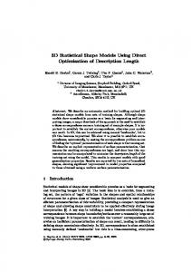
Since the shape space S is nonlinear, the definitions of sample statistics, such as means and covariances, are not conventional. Earlier papers [7, 8] suggest the use of Karcher mean to define mean shapes as follows. For α1 , . . . , αn in S, and d(αi , αj ) the geodesic length between αi and αj , the nKarcher mean is defined as the element µ ∈ S that minimizes the quantity i=1 d(µ, αi )2 . A gradientbased, iterative algorithm for computing the Karcher mean is presented in [8, 1]. Shown in Figure 1 are some examples of three classes of shapes – dogs, pears, and mugs – used in the experiments here, and the Figure 2 shows Karcher means of shapes in these three classes. Let µ be the mean shape and for any shape α, let g ∈ Tµ (S) be such that Ψ1 (µ; g) = α. Then, α called the exponential of g, i.e. expµ (g), and conversely, g = exp−1 µ (α). As described next, statistics of α are studied through statistics of its map onto the tangent space at the mean.

Fig. 1. Examples of three classes of shapes – dogs, pears, and mugs – from the ETH database that are studied in this paper, with the numbers used in test and training

3

Statistical Shape Models

Our goal is to derive and analyze probability models for capturing observed shapes. The task of learning probability models on spaces like S is difficult for two main reasons. Firstly, they are nonlinear spaces and therefore classical statistical approaches, associated with the vector spaces, do not apply directly. Secondly, these are infinite-dimensional spaces and do not allow component-by-component modeling that is traditionally followed in finite-dimensional vector spaces. The solution involves making two approximations. First, we project elements of S onto the tangent space Tµ (S), which is a vector space, and therefore, better suited to statistical modeling. This is performed using the inverse exponential map exp−1 µ . Second, we perform dimension reduction in Tµ (S) using PCA. Together,

616

A. Srivastava et al. 0.05

0.02

0.045

0.018

0.04

0.016

0.012

0.01

0.035

0.014

0.03

0.012

0.025

0.01

0.02

0.008

0.008

0.006

0.004 0.015

0.006

0.01

0.004 0.002

0.005 0

0.002

0

10

20

30

40

50

60

70

80

90

0

0

20

40

60

80

100

120

0

0

20

40

60

80

100

120

Fig. 2. In each case, left image shows the Karcher mean of shapes and right shows plots of the singular values of sample covariance matrix

these two approximations given rise to TPCA representation. These ideas were first proposed for landmark-based shape analysis in [6]. To start TPCA, we use the Gram-Schmidt algorithm to find an orthonormal basis of the given vectors: Set i = 1 and r = 1. i−1 1. Set Yi = gr − j=1 Yj , gr Yj . 2. If Yi , Yi = 0,  Set Yi = Yi / Yi , Yi , i = i + 1, r = r + 1, and go to Step 1. Else If r < k Set r = r + 1 and go to Step 1. Else Stop Say the algorithm stops at some i = n ≤ k. So now we have an n-dimensional subspace Y spanned by an orthonormal basis with elements {Y1 , Y2 , . . . , Yn }. The next step is to project each of the observed vector into Y as follows. Let xij = vector xi = [xi1 , xi2 , . . . , xin ] ∈ Rn . Then, the projection of gi , Yj and define a  n gi into Y is given by j=1 xij Yj . Each gi ∈ Tµ (S) is now represented by a smaller vector xi ∈ Rn . Next, we perform PCA in Rn using the projected observations {x1 , x2 , . . . , xk }. That is, from their sample covariance matrix C ∈ Rn×n , find its singular value decomposition C = U ΣU T , and use the first d-columns of U n to form a basis for the principal subspace of Rn , with d d ≤ n. The vector x ∈ R d maps to a smaller vector a ∈ R such that x = j=1 aj Uj . The choice of d is made using the singular values of C; shown in Figure 2 are the plots of singular values of C for the three classes: dogs, pears, and mugs. 3.1

Probability Models on TPCs

We impose a probability model on α implicitly by imposing a probability model on its tangent principal components (TPCs) a. What probability models can be used in this situation? In this paper, we study the following three models: nonparametric, Gaussian and mixtures of Gaussian. The first two models were studied for non-elastic shapes in [4]. 1. Nonparametric Model: Assuming that the TPCs, aj s, are statistically independent of each other, one can estimate their probability densities directly from (1) the data using a kernel estimator. Let fj , j = 1, . . . , d be the kernel estimate of the density function of aj , the j th TPC of the shape α. In the experiments presented here we used a Gaussian Kernel. Then, assuming independence of

Statistical Shape Models Using Elastic-String Representations

617

 TPCs, we obtain: f (1) (α) = dj=1 fj (aj ). Shown in Figure 3 are some examples of estimated f (1) for several js. For each shape class, we display three examples of non-parametric density estimates for modeling TPCs.

1.6

6

6

6

5

5

5

4

4

4

4

1.4

5 3 4

1

2.5

0.8

3

3

3

2

0.6

3

1.5 2

2

2

2

0.4

1 1

1

1

1

0.2

0 −1

6

3.5

1.2

0.5

−0.8

−0.6

−0.4

−0.2

0

0.2

0.4

0.6

0.8

1.8

0 −0.2

−0.1

0

0.1

0.2

0.3

0.4

0.5

6

0 −0.6

−0.5

−0.4

−0.3

−0.2

−0.1

0

0.1

0.2

0.3

4.5

1.6

0 −0.5

−0.4

−0.3

−0.2

−0.1

0

0.1

0.2

0 −0.4

4.5

4

4

4

3.5

3.5

3.5

−0.3

−0.2

−0.1

0

0.1

0.2

0.3

0.4

0.5

−0.1

0

0.1

0.2

0.3

0.4

0.5

6

5

5

1.4 1.2

0 −0.2

4

3

3

2.5

2.5

2

2

1.5

1.5

3 4 2.5

1 3

2

0.8

3

1.5 0.6

2

0.4

1

1

0.5

0.5

2 1

1

1

0.2 0 −0.8

−0.6

−0.4

−0.2

0

0.2

0.4

0.6

0.8

2.5

0 −0.2

−0.15

−0.1

−0.05

0

0.05

0.1

0.15

0.2

0.25

7

0 −0.5

−0.4

−0.3

−0.2

−0.1

0

0.1

0.2

0.3

0.4

0.5

0 −0.4

4.5

5

4

4.5

0.5

−0.3

−0.2

−0.1

0

0.1

0.2

0.3

0.4

2

0.4

0.6

−0.15

−0.1

−0.05

0

0.05

0.1

0.15

0.2

−0.1

−0.05

0

0.05

0.1

0.15

0.2

0.25

−0.2

−0.15

−0.1

−0.05

0

0.05

0.1

0.15

0.2

6

5

4 3 3

2

1

−0.2

−0.15

7

1

0.5 0 −0.4

0 −0.2

2

1 1

0.2

0.4

1.5

0.5

0

0.3

4

1.5

−0.2

0.2

2

2

−0.4

0.1

3 2.5

3

2.5

−0.6

0

3.5 3

4

0 −0.25

−0.1

4

3.5 5

0 −0.8

−0.2

5

2

1

−0.3

6

6

1.5

0 −0.4

1

0.5

−0.3

−0.2

−0.1

0

Dogs

0.1

0.2

0.3

0.4

0 −0.4

−0.3

−0.2

−0.1

0

0.1

0.2

0.3

0 −0.4

Pears

−0.3

−0.2

−0.1

0

0.1

0.2

0.3

0 −0.25

Mugs

Fig. 3. We show three examples of modeling TPCs in each class. For each example, the left figure shows nonparametric estimate f (1) while the right figure shows the mixture of Gaussian f (3) (using cross-lines) drawn over observed densities (plain lines).

2. Gaussian Model: Let Σ ∈ Rd×d be the diagonal matrix in SVD of C, the sample covariance of xi s. Then, we can model the  component aj as a Gaussian random variable with mean zero and variance Σjj . Denoting the Gaussian 1 exp(−(y − z)2 /(2σ 2 )), we obtain the density function as h(y; z, σ 2 ) ≡ √2πσ 2  d Gaussian shape model f (2) (α) = j=1 h(aj ; 0, Σjj ). 3. Mixture of Gaussian: Another candidate model is that aj follows the density  K d    (3) 2 pk h(aj ; zk , σk ) , pk = 1, fj (α) = j=1

k=1

k

a finite mixture of Gaussian. For a given K, EM algorithm can be used to estimate the means and variances of components. Based on empirical evidence, we have used K = 2 in this paper to estimate f (3) from observed data. Shown in Figure 3 are some examples of estimated f (3) for some TPCs. In each panel, the marked line shows the estimated mixture density and, for comparison, the plane line shows the observed histograms.

4

Empirical Evaluations

We have analyzed and validated the proposed shape models using: (i) random sampling, (ii) hypothesis testing, and (iii) statistics of log-likelihoods. We describe these results next.

618

A. Srivastava et al.

Fig. 4. Sample shapes synthesized from the nonparametric model (top) and the mixture model (bottom)

Shape Sampling: As a first step, we have synthesized random shapes from the three probability models f (i) , i = 1, 2, 3. In each case the synthesis involves generating a random TPC according to its probability model- kernel density, Gaussian density or mixture of Gaussian- and then reconstructing the shape represented by that set of TPCs. For the generated values n of TPCs, we form the d vector x = j=1 aj Uj , and the tangent direction g = i=1 xi Yi , and eventually the shape α = expµ (g). Shown in Figure 4 are examples of random shapes generated from the models f (1) (top row) and f (3) (bottom row). We found that all three models seem to perform reasonably well in synthesis, with f (1) and f (3) being slightly better than f (2) . Testing Shape Models In order to test proposed models for capturing observed shape variability, we use the likelihood ratio test to select among the candidate models. For a shape α ∈ S, the likelihood ratio under any two models is: (m) d  fj (aj ) f (m) (α) = , (n) f (n) (α) j=1 fj (aj )

m, n = 1, 2, 3 ,

and the log-likelihood ratio is l(α; m, n) ≡

d

 (m) (n) log(fj (aj )) − log(fj (aj )) . j=1

If l(α; m, n) is positive then the model m is selected, and vice-versa. Taking a large set of test shapes, we have evaluated l(α; m, n) for each shape and have counted the fraction for which l(α; m, n) is positive. We define: P (m, n) =

|{i|l(αi ; m, n) > 0}| , k

where k is the total number of shapes used in this test. This fraction is plotted versus the component size d in Figure 5, for two pairs of shape models: P (1, 3) in

Statistical Shape Models Using Elastic-String Representations 1

1

1

0.9

0.9

0.9

0.8

0.8

0.8

0.7

0.7

0.7

0.6

0.6

0.6

0.5

0.5

0.5

0.4

0.4

0.4

0.3

0.3

0.3

0.2

0.2

0.1

0.1

0

5

10

15

20

25

30

35

0

40

0.2 0.1

5

10

15

20

25

30

35

0

40

1

1

1

0.9

0.9

0.9

0.8

0.8

0.8

0.7

0.7

0.7

0.6

0.6

0.6

0.5

0.5

0.5

0.4

0.4

0.4

0.3

0.3

0.3

0.2

0.2

0.1

0.1

0

5

10

15

20

25

30

35

0

40

619

5

10

15

20

25

30

35

40

5

10

15

20

25

30

35

40

0.2 0.1

5

10

15

dogs

20

25

30

35

0

40

pears

mugs

Fig. 5. P (m, n) plotted versus vs d, for each of the three classes. Top row: m = 1, n = 3, and bottom row: m = 3, n = 2.

the top row and P (3, 2) in the bottom row. P (m, n) > 0.5 implies that model m outperforms n. Two sets of results are presented in each of these plots. The solid line is for the test shapes that were not used in estimation of shape models, and the broken line is for the training shapes that were used in model estimation. Also, we draw a line at 0.5 to clarify which model is performing better. As these indicate, the mixture model seems to perform the best in most situations. On the training shapes, for pears and mugs, the nonparametric model is better than the mixture model. This result in expected since nonparametric model is derived from these training shapes themselves. However, on the test shapes, the mixture model is either comparable or better than the other two models. We conclude that for this data set, the mixture model is better for capturing variability in both training and test shapes. Furthermore, it is efficient due to its parametric nature. Statistics of Model Likelihoods Another technique for model validation is to study the variability of a modelbased “sufficient statistic” when evaluated on both training and test shapes. In case the distributions of this statistic are similar on both training and test shapes, this validates the underlying model. In this paper, we have chosen the sufficient

0.14

0.12

0.1

0.14

0.12

0.12

0.09 0.12

0.12

0.1

0.1

0.1

0.08

0.08

0.06

0.06

0.08 0.1

0.1

0.07 0.08 0.06

0.08 0.06

0.08

0.05

0.06

0.06

0.04 0.04

0.04 0.03

0.04

0.04

0.04

0.02 0.02

0.02

0.02

0.02

0.02

0.01 0 −35

−30

−25

−20

−15

−10

dogs

−5

0 −50

−45

−40

−35

−30

−25

−20

−15

pears

−10

−5

0

0 −50

−45

−40

−35

−30

−25

−20

mugs

−15

−10

0 −35

−30

−25

−20

dogs

−15

−10

−5

0

0 −50

−45

−40

−35

−30

−25

−20

−15

pears

−10

−5

0

0 −50

−45

−40

−35

−30

−25

−20

−15

−10

mugs

Fig. 6. Histograms of ν (i) (α) for test (solid) and training shapes (broken). First three are for nonparametric model, and the last three are for mixture of Gaussians.

620

A. Srivastava et al.

statistic to be proportional to negative log-likelihood of an observed shape. That is, we define ν (i) (α) ∝ − log(f (i) (α)), where the proportionality implies that the constants have been ignored. Shown in Figure 6 are some examples of this study for the nonparametric (first three) and the mixture model (last three). These plots shows histograms of ν (i) (α) values for both test and training shapes, for each of the three shape classes. It is evident that the histograms for training and test sets are quite similar in all these examples, and hence, validate the proposed models. Acceptance/Rejection Under Learned Models: In the final experiment, we performed acceptance/rejection for each test shape under the mixture model, f (3) , for each shape class (dogs, pears, and mugs). Using threshold values estimated using training data of each class, we compute the value of ν (3) (α) for each test shape α; if it is below the threshold we accept it, otherwise we reject it. For example, we have dog reject > ν (3) (α) κdog . < dog accept This is done for each of the three classes – dogs, pears, and mugs, and the results are summarized in the next table. This table lists the percentage of times a shape from a given test class was accepted by each of the three shape classes. For example, test shapes in dog class were accepted 96.67% times by shape model for dog class, 1.67% by pear model, and 0.83% by cup model. Also, 1.67% of test shapes in dog class were rejected by all three models. Since a shape can be accepted by more than one model, the sum in each row can exceed 100%. Notice that the test shapes also include other objects such as horses, cows, apples, cars, and tomatoes. Some of the cows (35%) are accepted under dog model, but are easily rejected under pear and mug models; most of the cows (64%) are rejected under all three models. Tomatoes are mostly accepted by pear and mug models. Overall, the mixture model f (3) demonstrates a significant success in capturing shape variability and in discriminating between object classes. It also enjoys the efficiency of being a parametric model.

Test class Dog Dogs Pears Cups Horses Apples Cows Cars Tomatoes

Accepts (%) Pear 96.67 10.45 9.95 43.97 0 35.83 16.91 0.99

Accepts (%) Cups 1.67 99.00 28.35 0.00 78.71 0.00 0.99 67.66

Accepts (%) No Accepts (%) 0.83 1.67 41.79 0.99 98.01 1.49 0.52 56.02 96.53 0.99 0.00 64.17 46.76 38.30 72.13 19.90

Statistical Shape Models Using Elastic-String Representations

5

621

Conclusion

We have presented results from statistical analysis of planar shapes under elastic string models. Using TPCA representation of shapes, three candidate models were presented: nonparametric, Gaussian, and a mixture of Gaussian. We evaluated these models using (i) random sampling, (ii) likelihood ratio tests, (iii) similarity of (distributions of) sufficient statistics on training and test shapes, and (iv) acceptance/rejection of test shapes under the models estimated from the corresponding training shapes. All three models do reasonably well in random sampling and likelihood ratio test. However, the mixture model emerges as the best model for capturing shape variability and efficiency. We therefore conjecture that mixture of Gaussians are sufficient for modeling TPCs of observed shapes for use as prior shape models in future Bayesian inferences.

References 1. Klassen, E., Srivastava, A., Mio, W., Joshi, S.: Analysis of planar shapes using geodesic paths on shape spaces. IEEE Pattern Analysis and Machine Intelligence 26 (March, 2004) 372–383 2. Younes, L.: Optimal matching between shapes via elastic deformations. Journal of Image and Vision Computing 17 (1999) 381–389 3. Michor, P.W., Mumford, D.: Riemannian geometries on spaces of plane curves. Journal of the European Mathematical Society to appear (2005) 4. Srivastava, A., Joshi, S., Mio, W., Liu, X.: Statistical shape analysis: Clustering, learning and testing. IEEE Transactions on Pattern Analysis and Machine Intelligence 27 (2005) 590–602 5. Mio, W., Srivastava, A.: Elastic string models for representation and analysis of planar shapes. In: Proc. of IEEE Computer Vision and Pattern Recognition. (2004) 6. Dryden, I.L., Mardia, K.V.: Statistical Shape Analysis. John Wiley & Son (1998) 7. Le, H.L., Kendall, D.G.: The Riemannian structure of Euclidean shape spaces: a novel environment for statistics. Annals of Statistics 21 (1993) 1225–1271 8. Karcher, H.: Riemann center of mass and mollifier smoothing. Communications on Pure and Applied Mathematics 30 (1977) 509–541