Statistical voice activity detection based on integrated bispectrum likelihood ratio tests for robust speech recognition J. Ramírez,a兲 J. M. Górriz, and J. C. Segura Deptarment of Signal Theory, Networking and Communications, University of Granada, Granada, Spain
共Received 20 November 2006; revised 12 February 2007; accepted 13 February 2007兲 Currently, there are technology barriers inhibiting speech processing systems that work in extremely noisy conditions from meeting the demands of modern applications. These systems often require a noise reduction system working in combination with a precise voice activity detector 共VAD兲. This paper shows statistical likelihood ratio tests formulated in terms of the integrated bispectrum of the noisy signal. The integrated bispectrum is defined as a cross spectrum between the signal and its square, and therefore a function of a single frequency variable. It inherits the ability of higher order statistics to detect signals in noise with many other additional advantages: 共i兲 Its computation as a cross spectrum leads to significant computational savings, and 共ii兲 the variance of the estimator is of the same order as that of the power spectrum estimator. The proposed approach incorporates contextual information to the decision rule, a strategy that has reported significant benefits for robust speech recognition applications. The proposed VAD is compared to the G.729, adaptive multirate, and advanced front-end standards as well as recently reported algorithms showing a sustained advantage in speech/nonspeech detection accuracy and speech recognition performance. © 2007 Acoustical Society of America. 关DOI: 10.1121/1.2714915兴 PACS number共s兲: 43.72.Pf, 43.72.Dv 关EJS兴
I. INTRODUCTION
The emerging applications of speech technologies 共particularly in mobile communications, robust speech recognition, or digital hearing aid devices兲 often require a noise reduction scheme working in combination with a precise voice activity detector 共VAD兲.1 During the last decade numerous researchers have studied different strategies for detecting speech in noise and the influence of the VAD decision on speech processing systems.2–8 This task can be identified as a statistical hypothesis testing problem and its purpose is the determination to which category or class a given signal belongs. The decision is made based on an observation vector, frequently called feature vector, which serves as the input to a decision rule that assigns a sample vector to one of the given classes. The classification task is often not as trivial as it appears since the increasing level of background noise degrades the classifier effectiveness and causes numerous detection errors.9,10 The nonspeech detection algorithm is an important and sensitive part of most of the existing single-microphone noise reduction schemes. Well-known noise suppression algorithms11,12 such as Wiener filtering 共WF兲 or spectral subtraction, are widely used for robust speech recognition being the VAD critical in attaining a high level of performance. These techniques estimate the noise spectrum during nonspeech periods in order to compensate for the harmful effect of the noise on the speech signal. The VAD is even more critical for nonstationary noise environments since the statistics of the background noise must be updated. An example of
a兲
Electronic mail:
[email protected]
2946
J. Acoust. Soc. Am. 121 共5兲, May 2007
Pages: 2946–2958
such a system is the ETSI standard for distributed speech recognition that incorporates noise suppression methods. The so-called advanced front-end 共AFE兲13 considers an energybased VAD in order to estimate the noise spectrum for Wiener filtering and a different VAD for nonspeech frame dropping 共FD兲. On the other hand, a VAD achieves silence compression in modern mobile telecommunication systems reducing the average bit rate by using the discontinuous transmission mode. Many practical applications, such as the Global System for Mobile Communications 共GSM兲 telephony, use silence detection and comfort noise injection for higher coding efficiency. The International Telecommunication Union 共ITU兲 adopted a toll-quality speech coding algorithm known as G.729 to work in combination with a VAD module in DTX mode. The recommendation G.729 Annex B4 uses a feature vector consisting of the linear prediction spectrum, the fullband energy, the low-band 共0 – 1 kHz兲 energy, and the zerocrossing rate. Another standard for DTX is the ETSI 共adaptive multirate兲 AMR speech coder3 developed by the Special Mobile Group for the GSM system. The AMR standard specifies two options for the VAD to be used within the digital cellular telecommunications system. In option 1, the signal is passed through a filterbank and the subband energies are calculated. The VAD decision depends on a measure of the signal-to-noise ratio, the output of a pitch detector, a tone detector, and the correlated complex signal analysis module. An enhanced version of the original VAD is the AMR option 2 that uses parameters of the speech encoder that are more robust to the environmental noise than AMR1 and G.729. These VADs have been used extensively in the
0001-4966/2007/121共5兲/2946/13/$23.00
© 2007 Acoustical Society of America
open literature as a reference for assessing the performance of new algorithms. Most of the algorithms for detecting the presence of speech in a noisy signal only exploit the power spectral content of the signals and require knowledge of the noise power spectral density.6,8,14,15 One of the most important disadvantages of these approaches is that no a priori information about the statistical properties of the signals is used. Higher order statistics methods rely on an a priori knowledge of the input processes and have been considered for VAD since they can distinguish between Gaussian signals 共which have a vanishing bispectrum兲 from non-Gaussian signals. However, the main limitations of bispectrum-based techniques are that they are computationally expensive and the variance of the bispectrum estimators is much higher than that of power spectral estimators for identical data record size. These problems were addressed by Tugnait,16,17 who showed a computationally efficient and reduced variance statistical test based on the integrated polyspectra for detecting a stationary, nonGaussian signal in Gaussian noise. This paper shows an effective VAD based on a likelihood ratio test 共LRT兲 defined on the integrated bispectrum of the noisy speech. The proposed approach also incorporates contextual information to the decision rule, a strategy first proposed in Ref. 18 that has reported significant benefits for different applications including robust speech recognition.19–22 The paper includes a careful derivation of the LRT previously addressed in Refs. 23 and 24, an alternative approach based on block partitioning and averaging of the integrated bispectra, and its efficient implementation using the contextual LRT. The paper is organized as follows. Section II reviews the definition and fundamental properties of third-order cumulants and bispectrum. Section III suggests the use of integrated bispectrum for a reduced variance estimation while maintaining the benefits of higher order statistics for detection. Section IV shows the definition of the VAD based on contextual integrated bispectrum LRTs. Section V shows two different methods for integrated bispectrum estimation and LRT definition and their analysis and comparison is shown in Sec. VI. Section VII shows the receiver operating characteristic 共ROC兲 curves and speech recognition experiments that are used to evaluate the proposed method and to compare its performance to ITU-T G.729, ETSI AMR and AFE, as well as to other recently reported VADs. Finally, Sec. VIII summarizes the conclusions of this work.
=
冕
+⬁
x*共t兲x共t + 1兲x共t + 2兲dt
共2兲
−⬁
is the third-order cumulant of x共t兲, and = 2 f with normalized frequency f. By the symmetry properties, the bispectrum of a real signal is uniquely defined by its values in the triangular region 0 艋 2 艋 1 艋 1 + 2 艋 , provided that there is no bispectral alias. In a similar fashion, the bispectrum of a discrete-time signal is defined as the twodimensional 共2D兲 Fourier transform: ⬁
⬁
B x共 1, 2兲 =
兺 兺
C3x共i,k兲exp兵− j共1i + 2k兲其.
共3兲
i=−⬁ k=−⬁
Note that from the above-presented definition the third-order cumulant can be expressed as 1 共2兲2
C3x共i,k兲 =
冕冕
−
−
B x共 1, 2兲
⫻exp兵j共1i + 2k兲其d1d2
共4兲
using the inverse Fourier transform. Figure 1 shows the differences between cumulants and bispectrum function 共magnitude and phase兲 for a frame containing noise only 关Fig. 1共a兲兴 and speech in noise 关Fig. 1共b兲兴. Both data sets were extracted from an utterance of the Spanish SpeechDat-Car database27 with uniform noise conditions so that the noise level in both data sets is the same. It can be clearly concluded that higher order statistics or polyspectra provide discriminative features for speech/nonspeech classification.24 Even the bispectrum phase exhibits a more random behavior during nonspeech periods so that the phase entropy also provides complimentary information for VAD in noise environments.28 Although bispectrum methods have all the advantages of cumulants/polyspectra, their direct use has two serious limitations: 共i兲 The computation of bispectra in the whole triangular region is huge, and 共ii兲 the 2D template matching score in the classification is impractical. To efficiently use bispectra, integrated bispectrum methods16,17 were proposed for different applications.29,30
III. INTEGRATED BISPECTRUM
Let x共t兲 be a zero mean stationary random process. If we define ˜y 共t兲 = x2共t兲 − E兵x2共t兲其, the cross correlation between ˜y 共t兲 and x共t兲 is defined to be
II. BISPECTRUM
˜ 共t兲x共t + k兲其 = E兵x2共t兲x共t + k兲其 = C3x共0,k兲 r˜yx共k兲 = E兵y
The bispectrum of a deterministic, continuous-time signal x共t兲 is defined as25,26
冕 冕 +⬁
B共1, 2兲 =
C3x共1, 2兲 = E兵x*共t兲x共t + 1兲x共t + 2兲其
−⬁
so that its cross spectrum is given by ⬁
+⬁
C3x共1, 2兲
where J. Acoust. Soc. Am., Vol. 121, No. 5, May 2007
S˜yx共兲 = 兺 C3x共0,k兲exp兵− jk其
共6兲
冕
共7兲
−⬁
−⬁
⫻exp兵− j共11 + 22兲其d1d2 ,
共5兲
共1兲
and C3x共0,k兲 =
1 2
−
S˜yx共兲exp兵j共k兲其d .
Ramírez et al.: Statistical voice activity detection
2947
FIG. 1. Third-order statistics of: 共a兲 a noise only signal and 共b兲 a speech signal corrupted by car noise.
If we compare Eq. 共4兲 with Eq. 共7兲 we obtain S˜yx共兲 =
1 2
冕
−
Bx共, 2兲d2 =
1 2
冕
−
Bx共1, 兲d1 . 共8兲
2948
J. Acoust. Soc. Am., Vol. 121, No. 5, May 2007
The integrated bispectrum is defined as a cross spectrum between the signal and its square, and therefore a function of a single frequency variable. Hence, its computation as a cross spectrum leads to significant computational savings. But more important is that the variance of the estimator is of Ramírez et al.: Statistical voice activity detection
the same order as that of the power spectrum estimator. On the other hand, Gaussian processes have vanishing thirdorder moments so that the bispectrum and integrated bispectrum functions are zero as well. Section IV shows an innovative algorithm for voice activity detection taking advantage of the statistical properties of the integrated bispectrum. The proposed method is based on a LRT that can be evaluated using a Gaussian model for the integrated bispectrum of the signal.
presence of speech in the noisy signal. Thus, taking logarithms in Eq. 共10兲 and substituting the model defined in Eq. 共12兲 we obtain
冉
⌽共yˆ 兲 = 兺 log
=兺
再冉
p共Syx共兲兩H1兲 p共Syx共兲兩H0兲
冊
冊
冉 冊冎
1共 兲 0共兲 兩Syx共兲兩2 − log 1共 兲 0共 兲 0共 兲
1−
. 共13兲
Finally, if we define the a priori and a posteriori variance ratios as
IV. VOICE ACTIVITY DETECTION BASED ON THE INTEGRATED BISPECTRA
This section addresses the problem of voice activity detection formulated in terms of a classical binary hypothesis testing framework: H0 H1
: :
x共t兲 = n共t兲, 共9兲
x共t兲 = s共t兲 + n共t兲.
In a two-hypotheses test, the optimal decision rule that minimizes the error probability is the Bayes classifier. Given an observation vector yˆ to be classified, the problem is reduced to selecting the class 共H0 or H1兲 with the largest posterior probability P共Hi 兩 yˆ 兲. From the Bayes rule a statistical LRT 8 can be defined by L共yˆ 兲 =
py兩H1共yˆ 兩H1兲 py兩H0共yˆ 兩H0兲
共10兲
,
where the observation vector yˆ is classified as H1 if L共yˆ 兲 is greater than P共H0兲 / P共H1兲, otherwise it is classified as H0. In Ref. 22 the LRT first proposed by Sohn 8 for VAD, which was defined on the power spectrum, is generalized and extended to the case where successive observations yˆ 1 , yˆ 2 , . . . , yˆ m of the noisy signal are available. The so-called multiple observation LRT 共MO-LRT兲 reports significant improvements in robustness as the number of observations increases. This test involves evaluating the joint conditional distributions of the observations under H0 and H1, Lm共yˆ 1,yˆ 2, . . . ,yˆ m兲 =
py1,y2,. . .,ym兩H1共yˆ 1,yˆ 2, . . . ,yˆ m兩H1兲 py1,y2,. . .,ym兩H0共yˆ 1,yˆ 2, . . . ,yˆ m兩H0兲
which is easily performed if the observations are assumed to be independent. Assuming the integrated bispectrum 兵Syx共兲 : 其 as the feature vector yˆ and to be independent zero-mean Gaussian variables in the presence and absence of speech:
册 册
兩Syx共兲兩2 1 , exp − p共Syx共兲兩H0兲 = 0共 兲 0共 兲 p共Syx共兲兩H1兲 =
兩Syx共兲兩2 1 exp − , 1共 兲 1共 兲
兩Syx共兲兩2 0
共14兲
Eq. 共13兲 can be expressed in a more compact form:
冋冉 兺冋
⌽共yˆ 兲 = 兺
1−
=
冊
1 ␥共兲 − log共1 + 共兲兲 1 + 共兲
册
册
共兲␥共兲 − log共1 + 共兲兲 . 1 + 共兲
共15兲
Section IV A addresses two key issues in order to evaluate the proposed LRT: 共1兲 The estimation of the integrated bispectrum Syx共兲 by means of a finite data set, and 共2兲 the computation of the variances 0共兲 and 1共兲 of the integrated bispectrum under H0 and H1 hypotheses. A. Estimation of the integrated bispectrum Syx„…
Let Sˆyx共兲 denote a consistent estimator of Syx共兲 where Given a finite data set y共t兲 = x2共t兲 − E兵x2共t兲其. 兵x共1兲 , x共2兲 , . . . , x共N兲其 the integrated bispectrum is normally estimated by splitting the data set into blocks.25 Thus, the data set is divided into KB nonoverlapping blocks of data each of size NB samples so that N = KBNB. Then, the cross periodogram of the ith block of data is given by 共16兲
where X共i兲共兲 and Y 共i兲共兲 denote the discrete Fourier transforms of x共t兲 and y共t兲 for the ith block. Finally, the estimate is obtained by averaging KB blocks, K
1 B ˆ 共i兲 Sˆyx共兲 = 兺 S 共兲. KB i=1 yx
共17兲
This estimation is used to compute ␥共兲 through Eq. 共14兲. B. Computation of the variances 0„… and 1„ …
共12兲
the evaluation of the tests defined by Eqs. 共10兲 and 共11兲 only requires one to estimate the integrated bispectrum Syx共兲 of the noisy signal and variances 0 and 1 under absence and J. Acoust. Soc. Am., Vol. 121, No. 5, May 2007
␥共兲 =
1 共i兲 Sˆ共i兲 X 共兲关Y 共i兲共兲兴* , yx 共兲 = NB
, 共11兲
冋 冋
1共 兲 − 1, 0共 兲
共兲 =
The statistical properties of the bispectrum estimators have been discussed in Refs. 25 and 31. Thus, the test proposed Sec. IV A and the model assumed in Eq. 共12兲 are justified since for large NB, the estimates S共i兲 yx 共m兲 are complex Gaussian and independently distributed of S共i兲 yx 共n兲 for Ramírez et al.: Statistical voice activity detection
2949
m ⫽ n共m , n = 1 , 2 , . . . , NB / 2 − 1兲. Moreover, their mean and variance for large values of NB and KB can be approximated16 by E兵Sˆyx共兲其 ⬇ Syx共兲, 1 关Syy共兲Sxx共兲 + Re兵S2yx共兲其兴, var兵Re关Sˆ共i兲 yx 共兲兴其 ⬇ 2KB 1 关Syy共兲Sxx共兲 − Re兵S2yx共兲其兴, var兵Im关Sˆ共i兲 yx 共兲兴其 ⬇ 2KB 共18兲 where Re and Im denote the real and imaginary parts of a complex number. This means that, in order to estimate the variances 0 and 1 of the integrated bispectrum under the H0 and H1 hypotheses, we need to obtain an expression for Sxx共兲 and Syy共兲 when x共t兲 = n共t兲 共speech absence兲 and x共t兲 = s共t兲 + n共t兲 共speech presence兲, respectively. 1. Speech absence
Under the hypothesis H0, x共t兲 = n共t兲 and y共t兲 = x2共t兲 − E兵x2共t兲其. Thus, Sxx共兲 and Syy共兲 are reduced to Sxx共兲 = Snn共兲, Syy共兲 = Sn2n2共兲,
共19兲
where Sn2n2 can be expressed 共see the Appendix兲 by Sn2n2共兲 = 2Snn共兲 ⴱ Snn共兲 + 24n
共20兲
and 0 can be estimated by evaluating Snn共兲 and the variance of the noise: 0共 兲 =
1 关2Snn共兲 ⴱ Snn共兲 + 24n␦共兲兴Snn共兲. 共21兲 KB
FIG. 2. Estimation of Sss共兲 via smoothed spectral subtraction and Wiener filtering.
As a conclusion, a way to estimate the power spectrum of the clean signal Sss共兲 is needed for the evaluation of 1. A method combining Wiener filtering and spectral subtraction is used in this paper to estimate Sss共兲 in terms of the power spectrum Sxx共兲 of the noisy signal. The procedure is described as follows. During a short initialization period, the power spectrum of the residual noise Snn共兲 is estimated assuming a short nonspeech period at the beginning of the utterance. Note that Snn共兲 can be computed in terms of the DFT of the noisy signal x共t兲 = n共t兲. After the initialization period Sxx共兲 is computed for each frame through Eqs. 共16兲 and 共17兲 and Sss共兲 is then obtained by applying a denoising process. Denoising consists of a previous smoothed spectral subtraction followed by Wiener filtering. Figure 2 shows a block diagram for the estimation of the power spectrum Sss共兲 of the denoised speech through the noisy signal Sxx共兲. It is worthwhile clarifying that Snn共兲 is not only estimated during the initialization period but also updated during nonspeech frames based on the VAD decision. Thus, the denoising process consists of the following stages. 共1兲 Spectral subtraction: S1共兲 = LsSss共兲 + 共1 − Ls兲max共Sxx共兲 − ␣Snn共兲, Sxx共兲兲.
2. Speech presence
Under the hypothesis H1, x共t兲 = s共t兲 + n共t兲 and Sxx共兲 and Syy共兲 require a little more computation 共see the Appendix兲: Sxx共兲 = Sss共兲 + Snn共兲,
共22兲
By using Eq. 共20兲 for s共t兲 and substituting it in Eq. 共22兲 leads to 共23兲
Finally, 1共兲 can be estimated in terms of Sss共兲 and Snn共兲 by means of 1共 兲 =
2950
J. Acoust. Soc. Am., Vol. 121, No. 5, May 2007
S2共兲 = W1共兲Sxx共兲.
共26兲
共3兲 Second WF design and filtering:
W2共兲 = max共2共兲/共1 + 2共兲兲, 兲, Sss共兲 = W2共兲Sxx共兲,
共27兲 共−22/10兲
1 关Sss共兲 + Snn共兲兴关2Sss共兲 ⴱ Sss共兲 KB + 2Snn共兲 ⴱ Snn共兲 + 4Sss共兲 ⴱ Snn共兲兴.
1共兲 = S1共兲/Snn共兲,
2共兲 = S2共兲/Snn共兲,
Syy共兲 = 2Sss共兲 ⴱ Sss共兲 + 2Snn共兲 ⴱ Snn共兲 + 4Sss共兲 ⴱ Snn共兲.
共2兲 First WF design and filtering:
W1共兲 = 1共兲/共1 + 1共兲兲,
Syy共兲 = Ss2s2共兲 + Sn2n2共兲 + 4Sss共w兲 ⴱ Snn共兲 − 2共s4 + 4n兲␦共兲.
共25兲
共24兲
is selected to ensure a where Ls = 0.99, ␣ = 1, and  = 10 −22 dB maximum attenuation for the filter in order to reduce the high variance musical noise that normally appears due to rapid changes across adjacent frequency bins. The main reaRamírez et al.: Statistical voice activity detection
and 共24兲, respectively. Then, the a priori and a posteriori variance ratios 共兲 and ␥共兲, as defined in Eq. 共14兲, can be estimated and the VAD decision is obtained by comparing the LRT defined in Eq. 共15兲 to a given threshold . If the LRT is greater than the threshold the frame is classified as speech, otherwise it is classified as nonspeech. Finally, in order to track nonstationary noisy environments the power spectrum estimate of the noise is updated based on the current observation of the noisy signal: Snn共兲 = LnSnn共兲 + 共1 − Ln兲Sxx共兲
FIG. 3. Integrated bispectrum estimation by block averaging and VAD decision.
son for using a Wiener filter as noise reduction algorithm is found on its optimum performance for filtering additive noise in a noisy signal. This method is normally preferred to other conventional techniques such as spectral subtraction since the musical noise is significantly reduced as well as the variance of the residual noise. A two-stage Wiener filter configuration was used, as in the ETSI AFE standard,13 in order to make it less sensible to the VAD decision and the noise estimation process. V. DATA PROCESSING TECHNIQUES FOR VAD
The following shows the two different approaches for block managing that were used in this paper for the estimation of the integrated bispectrum of the input signal and its variances in the formulation of the LRT previously defined. A. Block partitioning and averaging
The first VAD method is described as follows. The input signal x共n兲 sampled at 8 kHz is divided into overlapping windows of size N = KBNB samples. A typical value of the window size is about 0.2 s, which yields accurate estimations of the integrated bispectrum. The best tradeoff between block averaging 共KB兲 and spectral resolution 共NB兲 will be discussed in the next sections. Figure 3 illustrates the way the signal is processed and the block of data the decision is made for. Note that the decision is made for a T-sample data block around the midpoint of the analysis window where T is the “frame-shift.” Thus, a large data set is used to estimate the integrated bispectrum Syx共兲 by averaging KB successive blocks of data while the decision is made for a shorter data set. As in most of the standardized VADs,3,4,13 the frame-shift is 80 samples so that the VAD frame rate is 100 Hz. After having estimated the power spectrum Sss共兲 of the clean signal through the denoising process shown earlier, the variances 0共兲 and 1共兲 of the integrated bispectrum under speech absence and speech presence are computed by evaluating the convolution operations required by Eqs. 共21兲 J. Acoust. Soc. Am., Vol. 121, No. 5, May 2007
共28兲
with Ln = 0.98 when the VAD detects a nonspeech observation. This method ensures a reduced variance estimation of the integrated bispectrum of the noisy signal by block averaging. However, the window shift T is typically much smaller than the block size and, therefore, the method is computationally expensive. In order to solve this problem, a computationally efficient but also effective method is developed in Sec. V B.
B. Contextual likelihood ratio test
Most VADs in use today normally consider hang-over algorithms based on empirical models to smooth the VAD decision. It has been shown recently21,22 that incorporating long-term speech information to the decision rule reports benefits speech/pause discrimination in high noise environments, thus making unnecessary the use of hang-over mechanisms based on hand-tuned rules. The VAD previously proposed addresses this problem by formulating a smoothed decision based on a large data set. However, an optimum statistical test involving multiple and independent observations of the input signal can be also defined as in Ref. 22 over the integrated bispectrum of the noisy signal using Eq. 共11兲. The proposed MO-LRT formulates the decision for the central frame of a 共2m + 1兲-observation buffer 兵yˆ l−m , . . . , yˆ l−1 , yˆ l , yˆ l+1 , . . . , yˆ l+m其: Ll,m共yˆ l−m, . . . , · yˆ l+m兲 =
pyl−m,. . .,yl+m兩H1共yˆ l−m, . . . ,yˆ l+m兩H1兲 pyl−m,. . .,yl+m兩H0共yˆ l−m, . . . ,yˆ l+m兩H0兲
,
共29兲 where l denotes the frame being classified as speech 共H1兲 or nonspeech 共H0兲. Note that, assuming statistical independence between the successive observation vectors, the corresponding log-LRT: l+m
ᐉl,m =
pyk兩H1共yˆ k兩H1兲
兺 ln p k=l−m
ˆ k兩H0兲 yk兩H0共y
共30兲
is recursive in nature, and if the ⌽ function is defined as ⌽共k兲 = ln
pyk兩H1共yˆ k兩H1兲 pyk兩H0共yˆ k兩H0兲,
共31兲
Eq. 共30兲 can be calculated as Ramírez et al.: Statistical voice activity detection
2951
integrated bispectrum Syx共兲 is estimated by averaging KB blocks using Eq. 共16兲 for each frame-shift T. This can be computationally expensive since the frame-shift is usually much lower than the window size 共N = KBNB兲. The second method based on the MO-LRT is more efficient since it just requires one to compute the integrated bispectrum of the current frame 共NB samples兲. The test is then built on a moving average fashion by means of Eq. 共32兲. This is clearly more efficient in terms of complexity since a single bispectrum computation is performed for each frame-shift T instead of the KB bispectrum estimations required by the first method. On the other hand, both methods exhibit high speech/nonspeech discrimination accuracy in noisy environments for equivalent delay configurations as will be shown in the following. FIG. 4. Operation of the MO-LRT VAD defined on the integrated bispectrum.
ᐉl+1,m = ᐉl,m − ⌽共l − m兲 + ⌽共l + m + 1兲.
共32兲
Now, if the integrated bispectrum of the noisy signal is considered as the feature vector, Eq. 共31兲 is reduced to be ⌽共k兲 = 兺
冋
册
k共 兲 ␥ k共 兲 − log共1 + k共兲兲 , 1 + k共 兲
共33兲
where k共兲 and ␥k共兲 denote the a priori and a posteriori variance ratios for the kth frame as defined in Eq. 共14兲. As a conclusion, the decision rule is formulated over a sliding window consisting of 共2m + 1兲 observation vectors around the frame the decision is made for. This fact imposes an m-frame delay to the algorithm that, for several applications, including robust speech recognition, is not a serious implementation obstacle. Figure 4 shows an example of the operation of the contextual MO-LRT VAD on an utterance of the Spanish SpeechDat-Car database.27 Figure 4 shows the decision variables for the tests defined by Eq. 共33兲 and, alternatively, for the test with the second log-term in Eq. 共33兲 suppressed 共approximation兲 when compared to a fixed threshold = 1.5. For this example, NB = 256 and m = 8. This approximation reduces the variance during nonspeech periods. It can be shown that using an eight-frame window reduces the variability of the decision variable yielding to a reduced noise variance and better speech/nonspeech discrimination. On the other hand, the inherent anticipation of the VAD decision contributes to reduce the number of speech clipping errors. The use of this test reports quantifiable benefits in speech/nonspeech detection as will be shown in Sec. VII. C. Comparison in terms of computational cost
It is interesting to compare the two methods proposed for voice activity detection based on single and multipleobservation LRTs. Both methods exhibit the advantages of VADs employing contextual information for formulating the decision rule since the decision variable is built on a longterm data set. The first method decomposes a large analysis window into KB blocks each of size NB samples and the 2952
J. Acoust. Soc. Am., Vol. 121, No. 5, May 2007
VI. ANALYSIS OF THE PROPOSED METHODS
In a Bayes classifier, the overlap between the distributions of the decision variable represents the VAD error rate.21 In order to clarify the motivations for the proposed algorithms, the distributions of the LRTs defined by Eqs. 共15兲 and 共30兲 were studied as a function of the design parameters KB, NB, and m. A hand-labeled version of the Spanish SpeechDat-Car database27 was used in the analysis. This database contains recordings from close-talking and distant microphones at different driving conditions: 共a兲 Stopped car, motor running, 共b兲 town traffic, low speed, rough road, and 共c兲 high speed, good road. The most unfavorable noise environment 共i.e., high speed, good road, and distant microphone兲 with an average SNR of about 5 dB was selected for the experiments. Thus, the decision variables defined by Eqs. 共15兲 and 共30兲 were measured during speech and nonspeech periods for the whole database, and the histogram and probability distributions were built. Separate results for each of the data processing techniques discussed previously are shown in the following. A. VAD based on block averaging
Figure 5 shows the distributions of speech and noise for different values of KB and NB. It is clearly shown that the distributions of speech and noise are better separated when increasing the number of blocks 共KB兲. When KB increases the noise variance decreases and the speech distribution is shifted to the right being more separated from the nonspeech distribution. Thus, the distributions of speech and nonspeech are less overlapped and consequently, the error probability is reduced. The reduction of the distribution overlap yields improvements in speech/pause discrimination. This fact can be shown by calculating the misclassification errors of speech and noise for an optimal Bayes classifier. Figure 5 also shows the areas representing the probabilities of incorrectly detecting speech and nonspeech and the optimal decision threshold. Figure 6 shows the independent decision errors for speech and nonspeech and the global error rate as a function of KB for NB = 256. The error rates were obtained by computing the areas under the class distributions of the decision variable shown in Fig. 5. The global error rate represents the Ramírez et al.: Statistical voice activity detection
FIG. 6. Probability of error as a function of KB for NB = 256.
total overlapped area while the speech and nonspeech error rate represent the areas below and above the optimum decision threshold, respectively. The speech detection error is clearly reduced when increasing the length of the window 共KBNB兲 while the increased robustness is only damaged by a moderate increase in the nonspeech detection error. These improvements are achieved by reducing the overlap between the distributions when KB is increased as shown in Fig. 5. It is interesting to show that the optimal values of the parameters KB and NB are conditioned to a fixed window size 共KBNB兲. This fact is shown in Fig. 7 where the minimum value of the global error rate depends on both NB and KB and is obtained for a typical window size of about 640–800 samples 共80– 100 ms兲. B. Integrated bispectrum MO-LRT VAD
Similar results were obtained for the MO-LRT VAD based on the integrated bispectrum of the noisy signal. Figure 8 shows the distributions of speech and noise for different values of KB and NB = 256. Again the noise variance decreases with m and the speech distribution is shifted to the
FIG. 5. Distributions of the decision variable for the VAD based on block averaging. 共a兲 NB = 64. 共b兲 NB = 128. 共c兲 NB = 256. J. Acoust. Soc. Am., Vol. 121, No. 5, May 2007
FIG. 7. Global error rates as a function of KB for NB = 64, 128, and 256. Ramírez et al.: Statistical voice activity detection
2953
FIG. 8. Distributions of the decision variable for the VAD based on MOLRT.
right. Figure 9 shows the independent decision errors for speech and nonspeech and the global error rate as a function of m for NB = 256. The total error is reduced with the increasing length of the window 共m兲 and exhibits a minimum value for a fixed order. According to Fig. 9, the optimal value of the order of the VAD is m = 6. Thus, increasing the length of the window is beneficial in high noise environments since the VAD introduces an artificial “hang-over” period which reduces front and rear-end clipping errors. This saving period is the reason for the increase of the nonspeech detection error shown in Fig. 9.
FIG. 9. Probability of error as a function of m for NB = 256.
A. ROC curves
The ROC curves are frequently used to completely describe the VAD error rate. They show the tradeoff between speech and nonspeech detection accuracy as the decision threshold varies.21 The AURORA subset of the original Spanish SpeechDat-Car database27 was used in this analysis. This database contains 4914 recordings using close-talking and distant microphones from more than 160 speakers. The
C. Concluding remarks
The two alternative methods for data processing and definition of the decision rule yield high discrimination accuracy and minimum global classification error rate for a given length of the analysis window. It can be concluded from Figs. 7 and 9 that the best results are obtained for a typical value of the window size of about 80– 100 ms. Thus, both methods benefit from using contextual information for the formulation of the decision rule. The VAD module then exhibits a delay of about half the length of the analysis window that for several applications including real-time speech transmission can be a serious implementation obstacle. However, for other applications including robust speech recognition, a delay of about 50– 80 ms in the VAD module does not represent a problem and can be accepted. VII. EXPERIMENTAL FRAMEWORK
Several experiments are commonly conducted in order to evaluate the performance of VAD algorithms. The analysis is mainly focused on the determination of the error probabilities or classification errors at different SNR levels6 and the influence of the VAD decision on the performance of speech processing systems.1 Subjective performance tests have also been considered for the evaluation of VADs working in combination with speech coders.32 The follwing describes the experimental framework and the objective performance tests conducted in this paper to evaluate the proposed algorithms. 2954
J. Acoust. Soc. Am., Vol. 121, No. 5, May 2007
FIG. 10. ROC curves obtained in high noise conditions. 共a兲 Block based integrated bispectrum LRT VAD. 共b兲 Integrated bispectrum MO-LRT VAD. Ramírez et al.: Statistical voice activity detection
TABLE I. Average word accuracy 共%兲 for the AURORA 2 for clean and multicondition training experiments. Results are averaged for all the noises and SNRs ranging from 20 to 0 dB.
WF WF+ FD WF WF+ FD
FIG. 11. Speech recognition experiments. Front-end feature extraction.
files are categorized into three noisy conditions: Quiet, low noisy, and highly noisy conditions, which represent different driving conditions with average SNR values between 25 and 5 dB. The nonspeech hit rate 共HR0兲 and the false alarm rate 共FAR0 = 100-HR1兲 were determined for each noise condition being the actual speech frames and actual speech pauses determined by hand-labeling the database on the close-talking microphone. Figure 10 shows the ROC curves of the proposed VADs and other frequently referred algorithms6,8,14,15 for recordings from the distant microphone in high noisy conditions. The working points of the G.729, AMR and AFE VADs are also included. Figure 10共a兲 shows how increasing the number of blocks 共KB兲 in the block averaging integrated bispectrum 共BA-IBI兲 LRT VAD leads to a shift-up and to the left of the ROC curve in the ROC space. This result is consistent with the analysis conducted in Figs. 5 and 7 that predicts a minimum error rate for KB close to five blocks. Similar results are obtained for the efficient MO-LRT IBI VAD that exhibits a shift of the ROC curve when the number of observations 共m兲 increases as shown in Fig. 10共b兲. Again, the results are consistent with our preliminary experiments and the results shown in Figs. 8 and 9 that expect a minimum error rate for m close to eight frames. Both methods show clear improvements in detection accuracy over standardized VADs and over a representative set of recently published VAD algorithms.6,8,14,15 Thus, among all the VADs examined, our VAD yields the lowest false alarm rate for a fixed nonspeech hit rate, and also the highest nonspeech hit rate for a given false alarm rate. The benefits are especially important over G.729, which is used along with a speech codec for discontinuous transmission, and over the algorithm of Li et al. 共Ref. 15兲, that is based on an optimum linear filter for edge detection. The
G.729
AMR1
AMR2
AFE
MO-LRT IBI
66.19 70.32 Woo 83.64 81.09
74.97 74.29 Li 77.43 82.11
83.37 82.89 Marzinzik 84.02 85.23
81.57 83.29 Sohn 83.89 83.80
84.15 85.71 Hand-labeled 84.69 86.86
proposed VAD also improves Marzinzik VAD6 that tracks the power spectral envelopes, and the Sohn VAD8 that formulates the decision rule by means of a statistical likelihood ratio test defined on the power spectrum of the noisy signal. It is worthwhile mentioning that the above-described experiments yield a first measure of the performance of the VAD. Other measures of VAD performance that have been reported are the clipping errors.32 These measures provide valuable information about the performance of the VAD and can be used for optimizing its operation. Our analysis does not consider or analyze the position of the frames within the word and assesses the hit rates and false alarm rates for a first performance evaluation of the proposed VAD. On the other hand, the speech recognition experiments conducted later on the AURORA databases will be a direct measure of the quality of the VAD and the application it was designed for. Clipping errors are indirectly evaluated by the speech recognition system since there is a high probability of a deletion error to occur when part of the word is lost after frame-dropping. B. Speech recognition experiments
Although the ROC curves are effective for VAD evaluation, the influence of the VAD in a speech recognition system was also studied. Many authors claim that VADs are well compared by evaluating speech recognition performance14 since nonefficient speech/nonspeech classification is an important source of the degradation of recognition performance in noisy environments.2 There are two clear motivations for that: 共i兲 Noise parameters such as its spectrum are updated during nonspeech periods being the speech enhancement system strongly influenced by the quality of the noise estimation, and 共ii兲 FD, a frequently used technique in speech recognition to reduce the number of insertion errors caused by the noise, is based on the VAD decision and speech misclassification errors lead to loss of speech, thus causing irrecoverable deletion errors. This section evaluates the VAD according to the objective it was developed for, that is, by assessing the influence of the VAD in a speech recognition system.
TABLE II. Average word accuracy 共%兲 for the Spanish SDC databases.
WM MM HM Avg.
Base
Woo
Li
Marz.
Sohn
G.729
AMR1
AMR2
AFE
MO-LRT IBI
92.94 83.31 51.55 75.93
95.35 89.30 83.64 89.43
91.82 77.45 78.52 82.60
94.29 89.81 79.43 87.84
96.07 91.64 84.03 90.58
88.62 72.84 65.50 75.65
94.65 80.59 62.41 74.33
95.67 90.91 85.77 90.78
95.28 90.23 77.53 87.68
96.39 91.75 86.65 91.60
J. Acoust. Soc. Am., Vol. 121, No. 5, May 2007
Ramírez et al.: Statistical voice activity detection
2955
Figure 11 shows a block diagram of the speech recognition experiments conducted to evaluate the proposed VAD. The reference framework 共base兲 considered for these experiments is the ETSI AURORA project for distributed speech recognition.33 The recognizer is based on the HTK 共Hidden Markov Model Toolkit兲 software package.34 The task consists of recognizing connected digits which are modeled as whole word HMMs 共Hidden Markov Models兲 with 16 states per word, simple left-to-right models, and three Gaussian mixtures per state 共diagonal covariance matrix兲. Speech pause models consist of three states with a mixture of six Gaussians per state. The 39-parameter feature vector consists of 12 cepstral coefficients 共without the zero-order coefficient兲, the logarithmic frame energy plus the corresponding delta and acceleration coefficients. Two training modes are defined for the experiments conducted on the AURORA-2 database: 共i兲 Training on clean data only 共Clean Training兲, and 共ii兲 training on clean and noisy data 共Multi-Condition Training兲. For the AURORA-3 SpeechDat-Car databases, the so called well-matched 共WM兲, medium-mismatch 共MM兲, and high-mismatch 共HM兲 conditions are used. These databases contain recordings from the close-talking and distant microphones. In WM condition, both close-talking and hands-free microphones are used for training and testing. In MM condition, both training and testing are performed using the hands-free microphone recordings. In HM condition, training is done using close-talking microphone recordings from all the driving conditions while testing is done using the hands-free microphone at low and high noise driving conditions. Finally, recognition performance is assessed in terms of the word accuracy 共WAcc兲 that considers deletion, substitution, and insertion errors. An enhanced feature extraction scheme incorporating a noise reduction algorithm and nonspeech FD was built on the base system.33 The noise reduction algorithm has been implemented as a single WF stage as described in the AFE standard13 but without mel-scale warping. No other mismatch reduction techniques already present in the AFE standard have been considered since they are not affected by the VAD decision and can mask the impact of the VAD precision on the overall system performance. Table I shows the recognition performance achieved by the different VADs that were compared. These results are averaged over the three test sets 共A, B, and C兲 of the AURORA-2 recognition experiments35 and SNRs between 20 and 0 dB. Note that, for the recognition experiments based on the AFE VADs, the same configuration of the standard,13 which considers different VADs for WF and FD, was used. The proposed integrated bispectrum MO-LRT VAD outperforms the standard G.729, AMR1, AMR2, and AFE VADs in both clean and multicondition training/testing experiments. When compared to recently reported VAD algorithms, the proposed one yields better results being the one that is closer to the “ideal” hand-labeled speech recognition performance. Table II shows the recognition performance for the Spanish SpeechDat-Car database when WF and FD are performed on the base system.33 Again, the VAD outperforms all the algorithms used for reference yielding relevant im2956
J. Acoust. Soc. Am., Vol. 121, No. 5, May 2007
provements in speech recognition. Note that these particular databases used in the AURORA 3 experiments have longer nonspeech periods than the AURORA 2 database, and then the effectiveness of the VAD results are more important for the speech recognition system. This fact can be clearly shown when comparing the performance of the proposed VAD to Marzinzik VAD.6 The word accuracy of both VADs is quite similar for the AURORA 2 task. However, the proposed VAD yields a significant performance improvement over Marzinzik VAD6 for the AURORA 3 database. VIII. CONCLUSIONS
This paper showed two different schemes for improving speech detection robustness and the performance of speech recognition systems working in noisy environments. Both methods are based on statistical likelihood ratio tests defined on the integrated bispectrum of the speech signal which is defined as a cross spectrum between the signal and its square, and inherits the ability of higher order statistics to detect signals in noise with many other additional advantages: 共i兲 Its computation as a cross spectrum leads to significant computational savings, and 共ii兲 the variance of the estimator is of the same order of power spectrum estimators. The proposed methods incorporate contextual information to the decision rule, a strategy that has reported significant improvements in speech detection accuracy and robust speech recognition applications. They differ in the way the signal is processed in order to obtain precise estimations of the integrated bispectrum and its variance. The optimal window size was determined by analyzing the overlap between the distributions of the decision variable and the error rate of an optimum Bayes classifier. The experimental analysis conducted on the well-known AURORA databases has reported significant improvements over standardized techniques such as ITU G.729, AMR1, AMR2, and ESTI AFE VADs, as well as over recently published VADs. The analysis assessed: 共i兲 The speech/nonspeech detection accuracy by means of the ROC curves, with the proposed VAD yielding improved hit rates and reduced false alarms when compared to all the reference algorithms, and 共ii兲 the recognition rate when the VAD is considered as part of a complete speech recognition system, showing a sustained advantage in speech recognition performance. ACKNOWLEDGMENTS
This work has received research funding from the EU 6th Framework Programme, under Contract No. IST-2002507943 共HIWIRE, Human Input that Works in Real Environments兲 and SESIBONN and SR3-VoIP projects 共Nos. TEC2004-06096-C03-00, TEC2004-03829/TCM兲 from the Spanish government. The views expressed here are those of the authors only. The Community is not liable for any use that may be made of the information contained therein. APPENDIX: VARIANCES OF THE INTEGRATED BISPECTRUM FUNCTION
This appendix demonstrates Eqs. 共20兲 and 共22兲 that were used in Sec. IV B for the computation of the variances 0共兲 Ramírez et al.: Statistical voice activity detection
and 1共兲 of the integrated bispectrum function under speech absence and speech presence, respectively. Let us assume the clean signal s共t兲 and the noise n共t兲 to be stationary, zero mean 共E关s共t兲兴 = E关n共t兲兴 = 0兲, statistically independent processes so that rx共k兲 = rs共k兲 + rn共k兲 ⇒ Sxx共兲 = Sss共兲 + Snn共兲,
共A1兲
where rx共k兲 denotes the autocorrelation function of the signal corrupted by additive noise. In order to derive the variances of the integrated bispectrum under the hypotheses H0 and H1, it is first needed to evaluate the autocorrelation function of the sequence y共t兲 = x2共t兲 − E关x2共t兲兴, which is defined as ryy共k兲 = E关y共t兲y共t + k兲兴 = E关共x2共t兲 − E关x2共t兲兴兲共x2共t + k兲 − E关x2共t + k兲兴兲兴.
+ E关x4兴E关x1x2x3兴兴 + 共− 1兲2共2!兲 ⫻关⫻E关x1兴E关x2兴E关x3x4兴 + E关x1兴E关x3兴E关x2x4兴 + E关x1兴E关x4兴E关x2x3兴 + E关x2兴E关x3兴E关x1x4兴 + E关x2兴E关x4兴E关x1x3兴 + E关x3兴E关x4兴E关x1x2兴兴 + 共− 1兲3共3!兲E关x1兴E关x2兴E关x3兴E关x4兴.
共A7兲
Note that Eq. 共A7兲 can be significantly reduced if the random variables are assumed to be zero mean: Cx1,x2,x3,x4 = E关x1x2x3x4兴 − 关E关x1x2兴E关x3x4兴 + E关x1x4兴E关x2x3兴 + E关x1x3兴E关x2x4兴兴.
共A8兲
Under the statistical independency assumption, the cross cumulants are null and the cross terms in Eq. 共A5兲 are reduced to
共A2兲 If the variance of the signal is defined as 2x = E关x2共t兲兴 = E关x2共t + k兲兴 then ryy共k兲 = E关共x2共t兲x2兲共t + k兲兴 − 4x .
共A3兲
Moreover, if the clean signal and the noise are assumed to be noncorrelated 共E关s共t兲n共t兲兴 = E关s共t兲兴E关n共t兲兴 = 0兲 the second term on the right-hand side of Eq. 共A3兲 can be expressed as
共A4兲 By defining ¯y 共t兲 ⬅ x2共t兲, Eq. 共A3兲 can be expressed as r¯y¯y共k兲 ⬅ E关共s共t兲 + n共t兲兲2共s共t + k兲 + n共t + k兲兲2兴 = E关s2共t兲s2共t + k兲兴 + E关n2共t兲n2共t + k兲兴 + E关s2共t兲n2共t + k兲兴 + 2E关s2共t兲n共t + k兲s共t + k兲兴 + E关n2共t兲s2共t + k兲兴 + 2E关n2共t兲n共t + k兲s共t + k兲兴 + 2E关n共t兲s共t兲s2共t + k兲兴 + 2E关n共t兲s共t兲n2共t + k兲兴 + 4E关n共t兲s共t兲n共t + k兲s共t + k兲兴,
共A5兲
where rs2s2 = E关s2共t兲s2共t + k兲兴 and rn2n2 = E关n2共t兲n2共t + k兲兴. Using the relation between fourth-order moments and cumulants given in Ref. 36 for a set or random variables: Cx1,. . .,xn =
兺 p ,. . .,p 1
⫻E
共− 1兲m−1共m − 1兲! m
冋兿 册 冋兿 册 i苸p1
Xi ¯ E
Xi ,
共A6兲
i苸pm
where 兵p1 , . . . , pm其 are all the partitions with m = 1 , . . . , n of the set of integers 兵1 , . . . , r其. In particular, for p = 4: 共A9兲
Cx1,x2,x3,x4 = 共− 1兲0共0!兲E关x1x2x3x4兴 + 共− 1兲1共1!兲 ⫻关E关x1x2兴E关x3x4兴 + E关x1x4兴E关x2x3兴 + E关x1x3兴E关x2x4兴 + E关x1兴E关x2x3x4兴 + E关x2兴E关x1x3x4兴 + E关x3兴E关x1x2x4兴 J. Acoust. Soc. Am., Vol. 121, No. 5, May 2007
Using these expressions, Eq. 共A5兲 is reduced to r¯y¯y共k兲 = rs2s2共k兲 + rn2n2共k兲 + 2s22n + rs共k兲rn共k兲
共A10兲
and Eq. 共A3兲 can be expressed as Ramírez et al.: Statistical voice activity detection
2957
ryy共k兲 = rs2s2共k兲 + rn2n2共k兲 + 4rs共k兲rn共k兲 − 共s4 + 4n兲. 共A11兲 Finally, the power spectrum of the squared centered signal y共t兲 is obtained after computing the discrete Fourier transform 共DFT兲 on Eq. 共A11兲: Syy共兲 = Ss2s2共兲 + Sn2n2共兲 + 4Sss共兲 ⴱ Snn共兲 − 2共s4 + 4n兲␦共兲,
共A12兲
where the asterisk “ⴱ” denotes convolution in the frequency domain. Finally, under speech absence x共t兲 = n共t兲 and assuming n共t兲 to be a Gaussian process:
共A13兲 or equivalently: Sn2n2共兲 = 2Snn共兲 ⴱ Snn共兲 + 24n␦共兲.
共A14兲
Note that, using the above-derived equations, the variances of the integrated bispectrum function under H1 and H0 hypotheses can be computed and the statistical tests used in the proposed VAD methods are completely described and justified. 1
R. L. Bouquin-Jeannes and G. Faucon, “Study of a voice activity detector and its influence on a noise reduction system,” Speech Commun. 16, 245–254 共1995兲. 2 L. Karray and A. Martin, “Towards improving speech detection robustness for speech recognition in adverse environments,” Speech Commun. 261– 276 共2003兲. 3 ETSI, “Voice activity detector 共VAD兲 for Adaptive Multi-Rate 共AMR兲 speech traffic channels,” ETSI EN 301 708 Recommendation, 1999 共European Telecommunications Standards Inst., France兲. 4 ITU, “A silence compression scheme for G.729 optimized for terminals conforming to recommendation V.70,” ITU-T Recommendation G.729Annex B, 1996 共International Telecomm. Union, Geneva兲. 5 A. Sangwan, M. C. Chiranth, H. S. Jamadagni, R. Sah, R. V. Prasad, and V. Gaurav, “VAD techniques for real-time speech transmission on the Internet,” in IEEE International Conference on High-Speed Networks and Multimedia Communications, 2002, pp. 46–50. 6 M. Marzinzik and B. Kollmeier, “Speech pause detection for noise spectrum estimation by tracking power envelope dynamics,” IEEE Trans. Speech Audio Process. 10, 341–351 共2002兲. 7 D. K. Freeman, G. Cosier, C. B. Southcott, and I. Boyd, “The voice activity detector for the pan-european digital cellular mobile telephone service,” in Proceedings of the International Conference on Acoustics, Speech and Signal Processing, 1989, pp. 369–372. 8 J. Sohn, N. S. Kim, and W. Sung, “A statistical model-based voice activity detection,” IEEE Signal Process. Lett. 16, 1–3 共1999兲. 9 I. Potamitis and E. Fishler, “Speech activity detection and enhancement of a moving speaker based on the wideband generalized likelihood ratio and microphone arrays,” J. Acoust. Soc. Am. 116, 2406–2415 共2004兲. 10 J. Górriz, J. Ramírez, J. C. Segura, and C. Puntonet, “An effective clusterbased model for robust speech detection and speech recognition in noisy environments,” J. Acoust. Soc. Am. 120, 470–481 共2006兲. 11 M. Berouti, R. Schwartz, and J. Makhoul, “Enhancement of speech corrupted by acoustic noise,” in Proceedings of the International Conference on Acoustics, Speech and Signal Processing, 1979, pp. 208–211. 12 S. F. Boll, “Suppression of acoustic noise in speech using spectral subtrac-
2958
J. Acoust. Soc. Am., Vol. 121, No. 5, May 2007
tion,” IEEE Trans. Acoust., Speech, Signal Process. 27, 113–120 共1979兲. ETSI, “Speech processing, transmission and quality aspects 共STQ兲; Distributed speech recognition; advanced front-end feature extraction algorithm; Compression algorithms,” ETSI ES 202 050 Recommendation, 2002 共European Telecommunications Standards Inst., France兲. 14 K. Woo, T. Yang, K. Park, and C. Lee, “Robust voice activity detection algorithm for estimating noise spectrum,” Electron. Lett. 36, 180–181 共2000兲. 15 Q. Li, J. Zheng, A. Tsai, and Q. Zhou, “Robust endpoint detection and energy normalization for real-time speech and speaker recognition,” IEEE Trans. Speech Audio Process. 10, 146–157 共2002兲. 16 J. K. Tugnait, “Detection of non-Gaussian signals using integrated polyspectrum,” IEEE Trans. Signal Process. 42, 3137–3149 共1994兲. 17 J. K. Tugnait, “Corrections to detection of non-Gaussian signals using integrated polyspectrum,” IEEE Trans. Signal Process. 43, 2792–2793 共1995兲. 18 J. Ramírez, J. C. Segura, M. C. Benítez, A. de la Torre, and A. Rubio, “A new adaptive long-term spectral estimation voice activity detector,” in Proceedings of EUROSPEECH 2003, Geneva, Switzerland, pp. 3041– 3044. 19 A. Sangwan, W. Zhu, and M. Ahmad, “Improved voice activity detection via contextual information and noise suppression,” in IEEE International Symposium on Circuits and Systems 共ISCAS兲, 2005, pp. 868–871. 20 J. Ramírez, J. C. Segura, C. Benítez, A. de la Torre, and A. Rubio, “An effective subband osf-based vad with noise reduction for robust speech recognition,” IEEE Trans. Speech Audio Process. 13, 1119–1129 共2005兲. 21 J. Ramírez, J. C. Segura, M. C. Benítez, A. de la Torre, and A. Rubio, “Efficient voice activity detection algorithms using long-term speech information,” Speech Commun. 42, 271–287 共2004兲. 22 J. Ramírez, J. C. Segura, C. Benítez, L. García, and A. Rubio, “Statistical voice activity detection using a multiple observation likelihood ratio test,” IEEE Signal Process. Lett. 12, 689–692 共2005兲. 23 J. Górriz, J. Ramírez, J. Segura, and C. Puntonet, “Improved MO-LRT VAD based on bispectra Gaussian model,” Electron. Lett. 41, 877–879 共2005兲. 24 J. Ramírez, J. M. Górriz, J. C. Segura, C. G. Puntonet, and A. Rubio, “Speech/non-speech discrimination based on contextual information integrated bispectrum LRT,” IEEE Signal Process. Lett. 13 共2006兲. 25 D. R. Brillinger and M. Rosenblatt, Spectral Analysis of Time Series 共Wiley, New York, 1968兲. 26 C. Nikias and M. Raghuveer, “Bispectrum estimation: A digital signal processing framework,” Proc. IEEE 75, 869–891 共1987兲. 27 A. Moreno, L. Borge, D. Christoph, R. Gael, C. Khalid, E. Stephan, and A. Jeffrey, “SpeechDat-Car: A large speech database for automotive environments,” in Proceedings of the II LREC Conference 2000. 28 J. M. Górriz, J. Ramírez, C. G. Puntonet, and J. Segura, “An efficient bispectrum phase entropy-based algorithm for VAD,” in Interspeech 2006, pp. 2322–2325. 29 X. Zhang, Y. Shi, and Z. Bao, “A new feature vector using selected bispectra for signal classification with application in radar target recognition,” IEEE Trans. Signal Process. 49, 1875–1885 共2001兲. 30 X. Liao and Z. Bao, “Circularly integrated bispectra: Novel shift invariant features for high-resolution radar target recognition,” Electron. Lett. 34, 1879–1880 共1998兲. 31 D. Brillinger, Time Series Data Analysis and Theory 共Holt, Rinehart and Winston, New York, 1975兲. 32 A. Benyassine, E. Shlomot, H. Su, D. Massaloux, C. Lamblin, and J. Petit, “ITU-T Recommendation G.729 Annex B: A silence compression scheme for use with G.729 optimized for V.70 digital simultaneous voice and data applications,” IEEE Commun. Mag. 35, 64–73 共1997兲. 33 ETSI, “Speech processing, transmission and quality aspects 共stq兲; distributed speech recognition; front-end feature extraction algorithm; compression algorithms,” ETSI ES 201 108 Recommendation, 2000 共European Telecommunications Standards Inst., France兲. 34 S. Young, J. Odell, D. Ollason, V. Valtchev, and P. Woodland, The HTK Book 共Cambridge University Press, New York, 1997兲. 35 H. Hirsch and D. Pearce, “The AURORA experimental framework for the performance evaluation of speech recognition systems under noise conditions,” in ISCA ITRW ASR2000 Automatic Speech Recognition: Challenges for the Next Millennium, Paris, France, 2000 共Intl. Speech Communication Assn.兲. 36 C. Nikias and A. Petropulu, Higher Order Spectra Analysis: a Non-linear Signal Processing Framework 共Prentice Hall, Englewood Cliffs, NJ, 1993兲. 13
Ramírez et al.: Statistical voice activity detection