Jan 21, 2010 - republish, to post on servers or to redistribute to lists, requires prior specific permission. ... These
Statistical Workloads for Energy Efficient MapReduce
Yanpei Chen Archana Sulochana Ganapathi Armando Fox Randy H. Katz David A. Patterson
Electrical Engineering and Computer Sciences University of California at Berkeley Technical Report No. UCB/EECS-2010-6 http://www.eecs.berkeley.edu/Pubs/TechRpts/2010/EECS-2010-6.html
January 21, 2010
Copyright © 2010, by the author(s). All rights reserved. Permission to make digital or hard copies of all or part of this work for personal or classroom use is granted without fee provided that copies are not made or distributed for profit or commercial advantage and that copies bear this notice and the full citation on the first page. To copy otherwise, to republish, to post on servers or to redistribute to lists, requires prior specific permission.
Statistical Workloads for Energy Efficient MapReduce Yanpei Chen, Archana Ganapathi, Armando Fox, Randy H. Katz, David Patterson RAD Lab, EECS Department, UC Berkeley 465 Soda Hall MS-1776 Berkeley, CA 94720
{ychen2, archanag, fox, randy, pattrsn}@eecs.berkeley.edu
ABSTRACT Energy efficiency is a growing concern in modern datacenters. As Internet services increasingly rely on MapReduce workloads to fuel their flagship businesses, there is a growing need for better MapReduce energy efficency evaluation mechanisms. We present a statistics-driven workload generation framework that distills summary statistics from production MapReduce traces and realistically reproduces representative workloads. These workloads help us evaluate design decisions with regard to scale, configuration, scheduling, and other issues. We use this framework to identify specific suggestions to improve MapReduce energy efficiency. Our key finding is that evaluations using trace-driven workloads reverse current design priorities in optimizing for data intensive synthetic jobs.
Categories and Subject Descriptors C.2.4 [Computer-Communication Networks]: Distributed Systems—Distributed applications
General Terms Measurement, Performance, Design, Economics
1. INTRODUCTION Energy consumption is an important factor in evaluating Internet datacenter efficiency. Over the lifetime of IT equipment, the operating energy cost is comparable to the initial equipment acquisition cost [10]. Also, datacenter operators recently showed that IT equipment power consumption dominates support facilities such as cooling and power distribution [2, 14, 16]. Datacenters are typically sized by their targeted power consumption, e.g. 1MW, 5MW, etc. Datacenters fully utilize their power supply by housing as much IT equipment and support facilities as limited by power consumption. As a result, companies must invest in new datacenter sites to handle growing computation needs instead of adding more machines to existing datacenters.
Many Internet enterprises have adopted the MapReduce computing paradigm to fuel many of their core businesses [12, 5]. The increasing popularity of MapReduce workloads necessitates a deeper understanding of their energy efficiency implications for datacenters. Existing efforts to evaluate MapReduce energy efficiency focus on data intensive jobs such as sort and the gridmix pseudo-benchmark [11, 15]. These approaches fail to capture a realistic mix of jobs, the range of data sizes, and the distribution of inter-job arrival times (Section 2). One of the factors preventing a more realistic MapReduce benchmark is the lack of publicly available production traces. Companies hesitate to publish their production traces due competitive concerns. Since different companies have very different MapReduce workload profiles (based on their usage scenarios), the absence of publicly available traces makes it difficult to construct a unifying, widely accepted benchmark. Even when production traces are available, MapReduce operators cannot monopolize production clusters for exploratory evaluation with regard to energy efficiency or other experimental design issues. A direct replay on a nonproduction cluster is also problematic, because it is difficult to reproduce the exact scale and hardware/software configuration profile of the production cluster, which makes design optimizations even more difficult to generalize. These concerns motivate the need for two tools – (1) a generalizable framework that allows production traces to be published in a sufficiently anonymous manner, and (2) a workload generator that effectively replays the statistical properties represented by the production traces. Our work suggests that trace analysis should be the starting point for any performance oriented work, including our specific focus on MapReduce energy efficiency. For the MapReduce example, we have a statistical framework that enables the publication of production traces in an anonymous fashion. In this paper, we demonstrate the success of this framework for guiding design decisions in energy efficient MapReduce. However, the framework is by no means limited only to energy efficiency optimizations. Our work hopefully encourages MapReduce operators to share traces, and enable researcher discoveries that have immediate impact. Against this backdrop, our contributions are as follows: 1. We analyze MapReduce production traces from a large Internet company. We build the case that it is essential
to know the mix of jobs, idle times, and data sizes. We also distill a sufficient and necessary set of statistical summaries that enables the publication of production traces in an anonymized fashion (Section 3). This section will also contain a brief overview of MapReduce. 2. We present a workload generation framework that takes as input the statistical summaries extracted from production traces. The workload generator accommodates differences in hardware, configurations, MapReduce implementation, cluster size, workload duration, and the actual computation being done in the original production trace (Section 4). Although our current implementation ignores the specific computation patterns of our workload to meet our anonymization goals, our design for the workload generator make it easily extensible to CPU, memory and I/O patterns if such data are available. 3. We evaluate several MapReduce energy efficiency mechanisms for our particular trace-driven workload. Our results show that prior design and evaluation approaches lead to the wrong design priorities (Section 5). 4. We reflect on the implications of our findings with regard to future methodology for distributed systems energy efficiency. We highlight several subtle methodological necessities that we hope would become standard evaluation practices (Section 6).
2. RELATED WORK In this section, we review several related and predecessor work. The take-away is that current studies in energy efficient MapReduce use pseudo-benchmarks that include a very small mix of jobs. As we will see in Section 3, existing approaches fail to capture production job diversity. SPEC power is an established benchmark for measuring system energy at different CPU utilizations [20]. A common methodology in software energy efficiency studies measures real-time CPU utilization, the power consumption at reference points obtained from SPEC power, and then approximate the real time whole system power by extrapolating CPU utilization from the reference points. The underlying assumption behind such extrapolation is that CPU is the dominant power consumer. Such approximation is invalid for workloads that involve a large amount of I/O activity, as in the case of MapReduce. Recent work showed that there would be significant discrepancies in the extrapolations unless we exercise all system resources in the correct mix when we measure SPEC power reference points. In distributed systems such as MapReduce, the extrapolation discrepancies would be multiplied across machines in the cluster, completely invalidating the method [17]. Power proportionality has been proposed as a worthy design goal [9]. Power proportionality differs from energy efficiency in that proportionality implies low energy consumption at low system utilization, and efficiency implies low energy usage to complete a certain compute job. Data intensive benchmarks emphasize efficiency over proportionality, since the system always performs compute tasks during energy measurement. A realistic job stream potentially contains many idle periods between job arrivals. Energy efficiency
during active periods would be insufficient if energy consumption during idle periods remain high. Thus, we need realistic workloads to study the right design point in both energy efficiency and power proportionality. JouleSort is a software energy efficiency benchmark that measures the energy required to perform an external sort [19]. The performance metric is energy per sorted record, with each record represented in standard terasort format with 10-byte keys and 90-byte data. Recent work in MapReduce energy efficiency also used the JouleSort benchmark, using clusters of tens of machines sorting 10-100GB data [11, 15]. Also, in work not related to energy efficiency, Yahoo! used the Hadoop implementation of MapReduce to sort petabyte scale data in reasonable time [21]. An increasingly frequent criticism is that JouleSort does not capture the mix of jobs and data patterns in production workloads. Thus, design choices guided by JouleSort may not be immediately usable in production. The gridmix pseudo-benchmark represents an improvement on sort [3]. The current version of gridmix contains five different jobs, each with different data ratios, that run on data sizes ranging from 500GB to a few GB. While gridmix contains more job types, it is still far from being representative of production workloads. We will do a more extensive comparison with gridmix during our discussion on trace analysis. The Mumak Hadoop simulator seeks to replicate the detailed behavior of a Hadoop cluster [6]. The design goal is to expedite evaluation and debugging of new mechanisms. Such simulators and our work complement each other. Using realistic workloads as simulator input, we can replicate cluster behavior under a production workload. A closely related work is [15]. The work seeks to improve HDFS energy efficiency by “sleeping” the nodes during periods of low load. This innovative idea exemplifies the shifting focus from active to idle energy in realistic workloads. However, the evaluation is still focused on sort and gridmix, and suffers a few methodological distractions such as using the CPU power interpolation method, evaluating only for default Hadoop configurations, and assuming sleeping nodes have zero power, which would not be true if the nodes still need to participate in data replication. We hope our contributions in the workload generator and methodological reflections would help fellow researchers make even greater contributions to the field. A direct predecessor to our work is [11]. The study looked at MapReduce energy consumption for a variety of jobs, stressing each part of the MapReduce data path. It examined design choices including cluster size, configuration parameters, and input sizes, to name a few. The remainder of this paper makes it evident that like other recent work on MapReduce energy efficiency, the exclusive focus on active energy for data intensive jobs fails to caputure the realistic behavior in production workloads. Another direct predecessor developed a multi-dimensional statistical method to accurately predict the execution time of MapReduce jobs [13]. The inputs to the prediction framework point to aspects of production traces worth capturing
to characterize a workload. Combining realistic workloads with accurate execution time predictions, we can implement mechanisms such as deadline schedulers and load sculpters, which would enrich the design space for energy efficient datacenter management.
3. TRACE ANALYSIS Before building a tool for realistic workload replay, we must first analyze production traces and identify necessary and sufficient information for realistic workload generation and replay. We obtained 6 months worth of MapReduce job history log traces from a production cluster at a large, wellknown Internet service. This production cluster represents a multi-user environment, running the Hadoop open source implementation of MapReduce on a cluster of hundreds of nodes. A brief overview of MapReduce is helpful at this point. At its core, MapReduce has two user-defined functions. The Map function takes in a key-value pair, and generates a set of intermediate key-value pairs. The Reduce function takes in all intermediate pairs associated with a particular key, and emits a final set of key-value pairs. Both the input pairs to Map and the output pairs of Reduce reside in an underlying distributed file system (DFS). The run-time system takes care of reading input from and writing output to the DFS, shuffling the intermediate data, scheduling and coordinating parallel execution, and handling machine failures.
Figure 1: CDF of inter-job arrival times for all jobs. The shaded circle represents the range of inter-job arrival times in sort and gridmix.
TB size workloads. When realistically replaying workload, we need to capture the entire range of data sizes to facilitate informed design decisions.
We can describe a single MapReduce job by several dimensions - the inter-job arrival time, the input, shuffle, and output data size, and the computation done for the map and reduce functions. A necessary and sufficient synthetic workload generator accurately captures the empirical mix of behavior, along these dimensions, for a large number of jobs. For some dimensions, a description using parametric statistics looks promising. For other dimensions, our analysis provides empirical evidence that parametric models are insufficient. We therefore identify necessary and sufficient non-parametric statistics to characterize MapReduce workloads. Figure 2: CDF of data sizes for all jobs. The shaded
3.1 Inter-Job Arrival Time Figure 1 shows the cummulative distribution function (CDF) of inter-job arrival times for our production trace, displaying the overall 6 months statistics and the statistics from two randomly chosen weeks. Most inter-job arrival intervals last as long as tens of seconds. In comparison, sort and gridmix launch jobs in quick succession with negligible inter-job arrival time, thus capturing only one extreme of the statistical distribution. The shape of the curves all indicate a Zipf-like distribution, suggesting that the trace is self-similar and captures a wide range of behavior over time.
3.2 Data Sizes The distribution of job data sizes is in Figure 2. The shape of the curves do not follow any well known parametric distributions. Further, we see that data sizes range from the KB scale to the TB scale. Again, sort and gridmix captures only an extreme end of the workload by using solely GB and
circle represents the range of data sizes in sort and gridmix.
3.3
Data Ratios
Since MapReduce jobs typically follow a three-stage execution pattern, another major factor that uniquely characterizes jobs is the data decrease (or increase) between the input, shuffle, and output phases. Figure 3 shows the distribution of shuffle-input, output-shuffle and output-input ratios for jobs in our workload. Similar to data sizes, non-parametric statistics would be more appropriate to summarize the distributions. Our production workload contains a substantial number of jobs that have hugely disproportionate input and output sizes. An example of data expansion jobs is reading a set of file pointers as input, and loading the contents of the file using MapReduce, resulting in a output data size many orders of magnitude larger than the input. An example of data aggregation jobs is computing the sum, or average of a
Figure 3: CDF of data ratios for all jobs. The shaded
Figure 5: CDF of input sizes for several frequent jobs.
rectangle represents the range of data ratios in sort and gridmix.
3.5
Sufficient Statistics
Our analysis of MapReduce trace characteristics strongly suggests the need for non-parametric statistical summaries to represent our production workload.
Figure 4: CDF of output/input data ratio grouped by 40th %tile in input size.
The simplest non-parametric statistics are average and standard deviation. It should be obvious from Figures 1 and 2 that the distributions are irregular, skewed, and asymmetric. Hence, averages and standard deviations are insufficient. Percentiles would give more or less an accurate description. However, the description may be overly accurate and raise data anonymity concerns. A good trade-off would be the five-number summary (1st, 25th, 50th, 75th, 99th percentiles). It captures the skew and dispersion of the data without making any assumptions about the underlying statistical distribution. The seven-number summary (2nd, 9th, 25th, 50th, 75th, 91st, 98th percentiles) also suffice, even though the choice of percentiles is based on a Gaussian model, i.e. the distance between the points would be regular if the distribution is Gaussian.
3.4 Per-Job Input Sizes
Also, data sizes is not necessary. In fact, divulging the full distribution of job data sizes may allow reverse engineering of the amount of computation on the cluster. Knowing the per node data size is enough, and we do not even need to know the cluster size. In addition to data anonymity concerns, when we replay the workload, we have to be agnostic to cluster size. The workload generator would be agnostic to cluster size if we replay using per node data size instead of per cluster data size, and scale the data size with the size of the cluster. Without this mechanism, workload replay would make little sense. It is meaningless to do on 10 node cluster a job as large as that done on a 1000 node cluster. The data simply would not fit in the available storage. Even if storage permits, the running time would be distorted by several orders of magnitude.
Figures 4 and 5 respectively show the CDF of output/input data ratio for big and small input jobs, and the input data size CDF for very frequent jobs in our production traces. These distributions are quite different from the CDF of all output/input data ratios in Figure 3 and the CDF of all input sizes in Figure 2. This suggests that there is a threeway dependency between the job, the distribution of its data sizes, and the distribution of its data ratios. Thus, our workload generation mechanism need to capture this dependency.
It would be straight forward to take the five-number summary of the overall inter-job arrival time and data sizes. However, doing so is still insufficient. We also need a way to identify different jobs. Any kind of unique ID would do, including ID by job name string comparisons. However, if the traces are anonymous, we would have no way of knowing the computation semantics of different job IDs. In particular, the unique ID could be numerical. Fortunately, since
large set of numerical values using MapReduce, resulting in a output data size many orders of magnitude smaller than the input. Existing sort and gridmix pseudo-benchmarks contain jobs with data ratios close to unity, and thus fails to accurately represent data expansion and data aggregation jobs. We believe these two types of jobs routinely appear in production MapReduce environments with big data processing needs. Thus, the empirical data again highlights the need for extracting representative distributions for each metric rather than focusing on a specific range of values.
we want the workload generator to anonymize the compute semantics anyway, we do not need to know the compute semantics at all. Also, we do not need to worry about different IDs aliasing to the same job. If we sample the frequency mix of jobs with the corresponding probability, we are guaranteed to get the right mix of data sizes regardless of redundant job ID aliases. Thus, the necessary and sufficient workload descriptor vector, used as input data to our workload generator, contains: 1. PDF of job frequency by job indices. 2. Five point summary (1st, 25th, 50th, 75th, and 99th percentiles) of inter job arrival rates. 3. For each job index, the five point summary of per-node input, shuffle and output data sizes. In general, trace analysis must distill what characteristics are important, what statistical summary is sufficient and necessary, and what are the dependencies between the characteristics. We know from a pre-release snapshot of Hadoop that the next version gridmix is starting to take on the trace-driven approach that we are advocating [8], although there are still major differences in the level of detail and anonymity that limits the extensibility and applicability of the pseudobenchmark. We have been in touch with our industry partners, and we are confident that our insights will contribute to an improved gridmix pseudo-benchmark.
4. WORKLOAD GENERATOR The workload generator comprises of two distinct components – (1) a mechanism to compose synthetic workloads from the trace-based five-number percentile summaries, and (2) a mechanism to replay the synthetic workload on a target platform. We discuss our design goals for the workload generation framework and describe the implementation of both components.
4.1 Design Goals We identified two main design goals for our workload generator. Our primary design goal is for our workload generation framework to be agnostic to hardware and software configuration, cluster size, and specific MapReduce implementation. It is unrealistic to expect access to production clusters to replay workloads. Not only would such access interfere with core business processes, but it would also restrict our evaluation to the specific configuration of the production cluster. The overhead of reproducing a production cluster’s hardware and software configurations, as well as reproducing the data layout and consequent skew, would impose signficant cost and effort. Thus, we must be able to replay our workload on a variety of platforms. This flexibility allows us to evaluate scale and configuration choices based on workload performance. A second design goals was to anonymize sensitive data in the traces by masking raw computation done by the jobs. Cap-
turing job-specific computations potentially reveals competitive core-business computations, and would prevent us from making our synthetic workload publicly available. Leaving out the compute portion of production jobs would allow us to compare workloads with different computations, thus creating a far more generic and widely applicable workload generation tool. Despite ignoring the compute part, we can still capture the essential characteristics of the jobs that facilitate configuration and trade-off design analysis. In the long term, we believe MapReduce type systems would become more IO bound, since CPU performance improves faster than IO performance. Thus, in the future, the cost ignoring compute would become progressively less. We later measure the cost of ignoring the compute component for present technology.
4.2
Trace Statistics to Synthetic Workloads
From our five-number summary statistics for each metric we collect for our jobs, we construct an approximate CDF for that metric by linearly extrapolating between the percentile metrics. We construct our synthetic workload by probabilistically sampling the approximated distributions per-metric and per-job. The sampling algorithm is as follows: 1. Sample the five-number summary-based CDF of job inter arrival times. 2. Sample the CDF of job indices. 3. For the job index obtained in Step 2, sample the five-number summary for the CDFs of per-node input data size, shuffle-input ratio, and output-shuffle ratio. 4. Construct vector [ inter job arrival time, job index, input data size, shuffle-input ratio, output-shuffle ratio ] and append to the workload. 5. Repeat until reaching the desired number of jobs or the desired workload time interval length. Thus, the synthetic workload would be a list of jobs described by [
inter job arrival time, job index, input data size, shuffle-input ratio, output-shuffle ratio ]
We can extend the algorithm in several ways. We can increase the sampling frequency of higher percentile values, to create a workload that emphasize data intense stress jobs. We can also customize the five-number summaries to investigate workloads with different statistical profiles. We can further plug-and-play the distributions from different organizations with completely different computation needs. In addition, we can create hypothetical future workloads by replacing the input summary statistics with manually created distributions. We see this extensibility as a step in the right direction towards evaluating cross-workload design decisions.
4.3 Realistic Workload Replay The primary objective for our framework is to enable realistic workload replay. To this end, we created a workload executor that takes our synthetically created workloads vectors and produces a sequence of MapReduce jobs with varying characteristics. At a high level, our workload generator consists of a shell script that launches jobs with specified data sizes and data ratios, and sleeps between successive jobs to account for inter-arrival times: HDFS randomwrite(max_input_size) sleep interval[0] RatioMapReduce inputFiles[0] \ output0 \ shuffleInputRatio[0] \ outputShuffleRatio[0] HDFS -rmr output0 & sleep interval[1] RatioMapReduce inputFiles[1] \ output1 \ shuffleInputRatio[1] \ outputShuffleRatio[1] HDFS -rmr output1 & ...
map(K1 key, V1 value, shuffle) { repeat floor(x) times { shuffle.collect(new K2(randomKey), new V2(randomValue)); } if (randomFloat(0,1) < decimal(x)) { shuffle.collect(new K2(randomKey), new V2(randomValue)); } } // end map() reduce(K2 key, values, output) { for each v in values { repeat floor(y) times { output.collect(new K3(randomKey), new V3(randomValue)); } } if (randomFloat(0,1) < decimal(y)) { output.collect(new K3(randomKey), new V3(randomValue)); } } // end reduce() } // end class RatioMapReduce
Our workload replay tool includes (1) a mechanism to populate the input data, (2) a MapReduce job that can adhere to specified input-shuffle and output-shuffle ratios, and (3) a mechanism to remove the MapReduce job output to prevent storage capacity overload. We discuss each of these three elements in turn. Populating data: We leverage the RandomWriter MapReduce job to write to HDFS the input data. This job creates a directory of fixed size files, each of which corresponds to the output of a reduce task. We need to populate the input data only once, writing enough data to account for the maximum input data size in our workload. All subsequent workload jobs can take as their input a random sample of these files, determined by their corresponding input data size. The input data size would have the same granularity as the file size, an inevitable tradeoff. We set each file to be 64MB, the same size as the default HDFS block size. We believe this setting is reasonable because our input files would be as granular as the underlying HDFS. Through experimentation, we also validated that there is negligible performance overhead when concurrent jobs reading from the same HDFS input. MapReduce job to preserve data ratios: We wrote a MapReduce job that reproduces job-specific shuffle-input and output-shuffle data ratios specified by the workload vector. Our implementation of this RatioMapReduce job uses a straightforward probabilitic identify filter: class RatioMapReduce { x = shuffleInputRatio y = outputShuffleRatio
Preventing HDFS storage overload: Lastly, we need a way to remove the data generated by the workload to avoid exceeding the storage capacity of our cluster. This mechanism is necessary because one could generate a workload with arbitrarily many jobs, which would certainly fill up any storage if the workload output is never removed. The mechanism we used was a straightforward HDFS remove command, issued to run as a background process while running the workload. We experimentally ensured that this mechanism imposes no performance overhead.
4.4
Acceptability of Ignoring Compute
A necessary step in anonymizing our trace data is to ignore specific job names and the computation they perform. While losing computation reproducibility does not impact our ability to evaluate design decisions, our replay accuracy may be impacted due to the absence of compute-bottlenecked jobs in the workload. Although we have sufficient evidence from job names in our traces to suggest that most MapReduce jobs are not compute-bottlenecked, we perform due diligence to justify that it is acceptable to ignore compute. We withhold publication of job names precisely due to anonymity concerns. We ran a MapReduce job that performed a word count on varying sizes of Wikipedia data loaded into our HDFS. Although word count is not the most compute-intensive example, it represents the higher end of computation performed in our production traces. Figure 6 compares the difference between performing the actual word count and running RatioMapReduce with the same data size. There is about 20% difference in duration and energy. The power consumed is virtually identical.
For batched execution, launch all jobs on the queue at the same time vs. in a staggered fashion: The master node is a single point of failure, and often becomes the bottleneck component of Hadoop. Launching jobs in a staggered fashion seeks to minimize additional inefficiencies in the Hadoop master, improving both energy and time efficiency. We implement staggered batch execution by inserting a sleep period of random length, between 0 and 20 seconds, at the start of each job launching thread.
Figure 6: Quantifying the cost of ignoring compute in wordcount.
To provide a more complete analysis, we also evaluate the cost of ignoring the computation on jobs known to be compute bound, such as calculating π using 18 map tasks, each doing 5,000,000,000 Monte-Carlo samples. Since our summary statistics make no effort to normalize for computation, our synthetically reproduced π has trivial data size, and the job completed in 23.6 seconds, compared to the actual compute π counterpart, which took almost 9 minutes to complete. The synthetic job consumed 1.33 joules per node compared to 99290 joules per node. Power consumption, on the other hand, differed by a mere 10 Watts. Thus, in the extreme worst case, discrepancies are significant, but they are easily prevented within our framework if the workload generator inputs also include job computation semantics.
5. ENERGY EFFICIENT MAPREDUCE In this section, we evaluate several MapReduce energy efficiency mechanisms, and discuss the implication of our results. The key lesson is that trace-driven workloads lead to different design priorities than many on-going efforts in optimizing MapReduce, for both energy and time efficiency.
5.1 Mechanisms Considered We look at design choices along four dimensions: Launch jobs as they arrive vs. queue up the jobs and launch them in batches: Most current systems are not power proportional. Thus, batched execution would lead to significant improvements in under-utilized clusters. We implement batched execution by launching the queued jobs using N threads, with each thread sequentially launching N1 of all jobs. In other words, the next job would not be launched until the previous job completes. Without this mechanism, if we launch all queued jobs simultaneously, the Hadoop master would be severely overloaded. To set N , we had to perform exploratory tuning. Too few threads would not fully occupy the cluster with active jobs while too many threads would slow down the Hadoop master. After trial and error, we found that a reasonable compromise is to set N to be the number of task trackers in the cluster.
Use the standard HDFS block size of 64MB vs. larger block sizes: We know from prior work that large HDFS block sizes results in faster finishing time and higher energy efficiency [21, 11]. If the cluster is highly utilized, large HDFS block sizes would result in significant improvements. We alter the HDFS block size by modifying the dfs.block.size parameter in the hadoop-site.xml configuration file. Assign the default 4 task trackers per node vs. more task trackers per node: If the per-node coordination overhead is low, having more task trackers per node would allow jobs to finish sooner. Given most current systems are not power proportional, finishing faster translates to lower energy consumption. We alter the task trackers per node by modifying the maximum map tasks and maximum reduce tasks parameters in the hadoop-site.xml configuration file. Our evaluation uses a day’s worth of generated workload. Running this workload under default settings would require a day. It takes significant time to perform repeated measurements for each mix of design choices, and it would be infeasible to scan the entire parameter space. Thus, we need to carefully select a few combinations of design choices to extract maximum insight from a minimum number of data points. We use the mix of design choices in Table 1. Using these configurations, we compare design choices in each dimension as follows: Batching vs. no batching - compare Configurations 1 and 2. Staggered launch vs. no staggered launch - compare Configurations 6 and 7. Large vs. small HDFS blocks - compare Configurations 2 and 4, or Configurations 3 and 6. Many vs. few task trackers per node - compare Configurations 2 and 3, or Configurations 4-6.
5.2
Cluster Setup
Our cluster has 10 nodes, each a Sun Microsystems X2200 M22 machine, with two dual-core AMD Opteron Processor 2214 at 2.2GHz, 3.80GB RAM, 250GB SATA Drive, running Linux 2.6.26-1-xen-amd64. Machines in the cluster connects to each other via 1Gbps Ethernet through a single switch. Each machine has approximately 150W fully idle power and 250W fully active power [7].
Table 1: Configurations for MapReduce workload energy measurements Configuration number 1 2 3 4 5 6 7
Batch? No Yes Yes Yes Yes Yes Yes
Staggered launch? N/A No No No No No Yes
Although a cluster of 10 nodes appears small for our experiments, a survey of production clusters at a diverse collection of enterprises suggest that around 70% of MapReduce clusters contain fewer than 50 machines [5]. Thus, our findings on 10 machines easily generalize to clusters at that scale. Only a handful of large Internet enterprises have clusters with more than hundreds or thousands of machines. The scale of large production clusters are hard to accurately replicate. Our workload preserves the per-node data intensity, enabling designers to evaluate mechanisms on production size clusters if such resources are available. We use the Hadoop implementation of MapReduce [4]. We use Hadoop distribution 0.18.2 running on Java version 6.0, update 11. We decided against newer distributions to ensure data comparability with our early experiments and the results in [11]. Unless otherwise noted, we used default configuration parameters for Hadoop. We run experiments in a controlled environment. Because we use a shared cluster and cannot guarantee that absence of background tasks on the machines we used, we perform our experiments during periods of low or no background load on the cluster. We closely monitor the CPU, disk, and network load during our experiments. When we detect any activity not due to Hadoop, we stop data collection and repeat the measurement at a later time. We run Hadoop with no virtualization. A subject of future work is to extend our workload generation framework to incorporate realistic non-MapReduce background loads.
5.3 Energy Measurement Method
HDFS block size 64MB 64MB 64MB 80MB 80MB 80MB 80MB
Task trackers per node 4 4 8 4 6 8 8
the exact data and computation on which the jobs were run. Anonymized trace would not contain this information. Thus, given anonymity limitations and the randomized nature of Hadoop scheduling and block placement algorithms, we need to monitor only one worker, and capture the variation between workers by taking repeated measurements. We use a Brand Electronics Model 21-1850/CI power meter. It has 1W power resolution with logging capabilities, and we set it to sample at 1Hz.
5.4
Results
Figure 7 shows the results of our experiment. The table shows raw numerical values for duration, energy, and average per node active power. The graph shows normalized values, with Configuration 1 being the baseline. The error range in the table and error bars in the graph represent 95% confidence intervals from 3 repeated runs. We did not do more repeated runs to narrow the confidence intervals further because each run of the workload takes a long time, and we are limited by the availability of the shared cluster. In our experience, variability increases with cluster size, since there is a greater probability of data skews and network bottlenecks. Thus, variability will likely increase when we scale our experiments to clusters of hundreds or even thousands of nodes. Since we are interested in energy efficiency, our primary performance metric is the energy consumed. Using this metric, design choices in the four dimensions are resolved below.
We measure energy at the wall power socket. As a result, the power-energy measurements capture the holistic system performance, including any components that may be idle and drawing wasted power.
Batching causes up to an order of magnitude decrease in duration and energy, for a modest increase in per node average power. We see this by comparing Configuration 1 with all the other configurations.
We make several methodological simplifications. Ideally, measurements should include the MapReduce master, all MapReduce workers, and the network switch. As we found in [11], including the master in power energy measurements distorts data trends for small clusters, since the energy consumption of the master amortizes across increasing cluster size. So a larger cluster would appear to have better energy efficiency simply by amortizing the fixed MapReduce master overhead. Monitoring the network switch is problematic for the same reason. Furthermore, for a homogenous cluster not optimized for rack locality, the behavior of one worker is statistically identical to the behavior of other workers. Additionally, reproducing data skew is unrealistic without
Staggered launch of batched jobs lead to no statistically significant improvement, since Configurations 6 and 7 have overlapping 95% confidence intervals in energy consumption. However, the average energy of Configuration 7 is lower. Larger HDFS blocks lead to statistically significant improvements when there are 8 task trackers per node. This fact is evident by Configuration 6 having a lower energy consumption than Configuration 3, with non-overlapping confidence intervals. However, at 4 task trackers per node, the choice of HDFS block size leads to no significant energy decreases, evident from the heavily overlapping confidence intervals of Configurations 2 and 4.
Figure 7: Performance of different MapReduce optimization mechanisms. In the graph, the raw values are normalized with Configuration 1 being the baseline. See Table 1 for details of each configuration.
More task trackers per node lead to a performance penalty with 64MB HDFS blocks, evident from the higher average energy of Configuration 3 compared with Configuration 2, with non-overlapping confidence intervals. However, at 80MB HDFS blocks, the energy variations are not statistically significant. We interpret the results with regard to HDFS block size and task trackers per node to indicate that there are nonnegligible coordination overheads when there are a large number of concurrent tasks. Along both design dimensions, the performance penalty is visible only when compared with Configuration 3, which has 8 task trackers per node and small HDFS blocks. This configuration produces the largest number of concurrent tasks, since there is one map task for each HDFS block in the input, and the number of reduce tasks is fixed. The slowdown is caused by the Hadoop master coordinating task states across the cluster. Because small HDFS blocks do not affect the maximum number of concurrent tasks on a single node, the per node coordination overhead remains fixed, and thus Hadoop workers are not the cause of the slowdown. Collectively, the results show that for the particular workload we analyzed, batching leads to significant first order improvements. Once we harness the first order improvements, further optimizations are difficult to achieve.
5.5 Discussion Our results suggest that we should not launch MapReduce jobs as they arrive, but queue the incoming jobs, and launch them in regular batched fashion. As a result, we can turn off the entire cluster, between batch intervals, when all jobs in a batch complete. This mechanism allows us to achieve energy proportionality through workload management and application scheduling, even in the absence of energy proportional hardware. If we want to deploy a batch MapReduce scheduler, the batch interval duration is an important concern. First, the batch interval length must be longer than the time it takes to bring up and shut down a MapReduce cluster. Second, the batch interval must be long enough to ensure that there are enough jobs on queue to fully utilize the cluster. Third,
the batch interval must not be so long that applications consuming MapReduce outputs would be severely impacted. An additional concern is whether we increase hardware failure probability if we frequently turn on and turn off clusters. Recent estimates suggest that over the lifetime of equipment, both disk storage and integrated circuits can sustain power cycle frequency as high as one per hour. An ongoing 18 month experiment on a research cluster at the Information Science Institute (ISI) suggests that turning off nodes after one hour of idleness has no impact on hardware reliability [18]. Thus, until new empirical data suggests otherwise, we believe turning off entire clusters would not hurt hardware reliability. Furthermore, cluster idling between batches of workloads is an undesirable property despite minimal energy consumption. To compensate for the upfront cost of cluster equipment, already paid for by the organization, it is more desirable to keep the cluster active with useful work. In the extreme case, if the cluster is almost always idle, one could conclude that the cluster was over-provisioned, perhaps to handle hypothetical peak demand. One solution is to offer several different service levels, one for immediate job launch, one for frequent batchs on the order of minutes, one for regular batches on the order of hours, and another for daily batches. With such a service model, we can develop additional insight with regard to the volume of jobs suitable for each class of batch workload. With this insight, we can assign different batch service models to different clusters, and size each cluster for high utilization at all times. Another mechanism already in use in some large datacenters is to mix interactive and batch jobs in the same cluster. By appropriately controlling batch intervals, one can completely shape the volume of actively running batched jobs. In particular, one can shape batch job volume to match any diurnal patterns in interactive jobs. This mechanism also ensures that the cluster sustains high utilizations. A more fundamental way to increase cluster utilization is to develop new business processes that extract value from
additional cluster usage. Once the cluster utilization is high, the focus shifts from energy proportionality back to energy efficiency. Having realistic workloads would allow us to further explore design choices at high cluster utilization levels. Our data also informs discussions on hardware energy proportionality. The hardware in our cluster is highly power disproportional. The average per node power at high utilization (Configurations 2-7) is nearly the same as per node power at low utilization (Configuration 1). With highly power disproportional hardware, improving time efficiency is frequently a proxy for improving energy efficiency, since energy is the product of time and power, and power is approximately constant. When hardware becomes power proportional, low cluster utilization would waste the investment in equipment, and there would be zero power consumption when the cluster is idle. That said, energy efficiency would continue to be important as higher efficiency would still allow us to do the same computation with lower energy cost. Most importantly, the discussion here is completely concerned with workload level optimizations, which is a fundamental shift from individual job level optimizations. Thus far, job level optimizations drives work in both MapReduce energy efficiency [11, 15] and MapReduce time efficiency [23, 22]. This trend is mostly an artifact of the exclusive focus on sort and gridmix as evaluation tools. Both measure per job performance at high data intensities. Since most clusters are currently provisioned for peak usage rather than average usage, clusters are under-utilized. Consequently, work on improving configurations, scheduling, data locality may entirely miss the point because such optimizations are relevant only when the cluster is active. Based on our findings, we argue for a change in research focus from job level optimizations to workload level optimizations.
6. METHODOLOGY REFLECTIONS The experience and results from our energy efficiency case study revealed insights on subtle methodological necessities of distributed system energy efficiency studies. We share our insights below in the hope that they will help future work obtain high quality results. Energy is the right metric; power is the wrong one. Figure 7 clearly distinguishes between energy and power. If we had optimized for low power, then Configuration 1 would perform the best, even though the energy consumption is much higher due to longer workload duration. In the extreme case, a machine that computes arbitrarily slowly by being idle would have the active power equivalent to idle power. Obviously, since idle power is lower than non-idle machine power, the duration, and hence energy, would be infinite. Power meters are necessary. High quality power meters represent a non-negligible investment and are not yet a widespread research, let alone pro-
duction, tool. In the absence of power meters, one alternative is to use SPECpower measurements coupled with CPU extrapolations, already explained to be insufficient in Section 2. Another alternative is to assume name-plate power or constant average power, and use duration as a proxy for energy. The assumption of constant average power hardly ever holds, even if the dynamic power range is small. For the machines in our cluster, the dynamic power range is 40% of name-plate power. This range compounds the roughly 40% variation in job duration in Figure 7. Thus, without a power meter, an energy by duration estimate could be as low as 36% or as high as 196% of the actual value. Also, we were fortunate that our Hadoop job durations were on the order of seconds and even minutes, and the dynamic power range of our machines are on the order of tens of Watts. Consequently, we were able to use power meters with 1W resolution and 1Hz sampling rate. This class of equipment is still reasonably easy to find. If we were to tackle per-component power studies at the hardware level, the events would have durations on the order of microseconds, and dynamic power range could possibly go as low as a few mW. Such studies would require power meters of an even higher caliber. Overall, high quality power meters represent a necessary investment for research groups interested in computer systems energy efficiency. Repeated measurements are necessary. Our results in Figure 7 show that the duration and energy for Configurations 2, 4, 5, 6, 7 are statistically identical. However, if we had taken only one measurement for each configuration, then we would incorrectly conclude that some of these configurations are better than others. Thus, while repeated measurements are standard good experimental practices, they are essential in distributed systems performance measurements. For our repeated measurements, we compute 95% confidence intervals by assuming the underlying statistical distribution to be Gaussian. This practice is common and we explain why it is statistically sound. We can assume the underlying distrbution is Gaussian using the Central Limit Theorem. This theorem states that the sample mean of a large number of independent, identically distributed random variables with finite mean and variance would approach a Gaussian distribution. For repeated measurements, each measurement corresponds to sampling the random variable that represents the performance of the underlying system. This random variable has finite mean and variance because the system performance has finite mean and variance. Thus, if we assume that each measurement is independent, and the underlying system has the same performance distribution between measurements, then the premises in the Central Limit Theorem hold, and the distribution of the sample mean converges to a Gaussian for a large number of samples. By the BerryEsseen Theorem, √ in the worst case, the convergence error decreases at O(1/ n), where n is the number of samples. With the Gaussian √ assumption, confidence intervals also decrease at O(1/ n). Thus, for a given confidence level, halv-
ing the confidence interval would require taking four times as many measurements. Conversely, for the same number of measurements, the width of confidence intervals increases inversely to the Gaussian CDF of the associated confidence levels. A helpful numerical example is at [1]. Small improvements difficult to justify for highly variable systems. This fact is a direct consequence of the statistical properties of confidence intervals. Intuitively, we can arbitrarily narrow confidence intervals by taking arbitrarily many measurements. To validate improvements in a statistically sound manner, we need non-overlapping confidence intervals, which would require many measurements if the size of the improvements is less than the performance variation of the underlying system. At such design points, it becomes debatable whether we should prioritize improving the mean performance or decreasing the performance variation. To use a concrete example, suppose we are trying to verify a 20% improvement for a system with performance standard deviation that is 30% of the mean, which is comparable to the average performance standard deviation for Configurations 2-7 in Figure 7. For non-overlapping confidence intervals, we need to narrow the confidence interval to ±10% of the mean, which is half of the fraction of improvement. At the 95% confidence level, this resolution requires approximately 35 measurements to achieve. Thus, reducing performance variance from 40% to 20% may be a higher design priority than improving average performance by 20%. The performance variations we observed are typical to systems like MapReduce. Thus, improvements on the order of a few tens of percent are difficult to statistically justify. Fortunately, our primary improvements in Figure 7 are an order of magnitude instead of a few tens of percent. Need per-workload performance metrics. Prior work in JouleSort [19] introduced per-job energy efficiency metrics such as joules per sorted record. However, once we shift the design focus from job level decisions to workload level optimizations, we need per-workload energy efficiency metrics, since per-job metrics only measures energy efficiency for the active portion of the workload. In our study, we avoided this issue by using the same workload for evaluating design choices. We believe it is nontrivial to develop good workload metrics because a workload has many more characteristics than a job. For example, while the joules per sorted record metric applies to sort jobs regardless of data size and sorting algorithm, it would be difficult to develop a “joules per something ” metric for workloads with different durations, number of jobs, data sizes, and mix of computations. That said, just as the JouleSort metric continues to drive job level energy efficiency improvements, a good metric for workload energy efficiency would be vital for workload level optimizations.
7. FUTURE WORK We see several future uses for our MapReduce workload generator as well as the more general trace-driven statistical
framework. Both have applications outside energy efficiency. We group future work under two sections - capabilities immediately enabled by having realistic workloads, and long term applications of our approach.
7.1
Immediate Enablers
The immediate implications of our analysis suggest that prior work on MapReduce scheduling results in far less performance gains compared to batching workloads and running them periodically. This result makes a case for research on deadline-driven scheduling, where jobs with relaxed deadlines can run in batches at convenient times instead of being serviced upon arrival. The anonymization properties of our framework are essential for alleviating privacy concerns that have thus far prevented organizations from sharing their production traces. Using five-number summary statistics, we effectively capture the variability in workload characteristics while abstracting away sensitive information. We believe this methodology enables us to compare workloads across organizations, which will eventually lead to a more widely accepted MapReduce benchmark. We are in the process of aquiring traces from other MapReduce production environments and plan to use summary statistics to make them publicly available. While our five-number summary percentiles are based on traditional statistical techniques for summarizing distributions, we believe the systems community will find value in focusing on percentile values higher than the 99th. Data that exceeds the 99th percentile potentially represents worst case behavior. System developers would benefit from understanding their system’s performance under unusually high load as it enables them to evaluate mechanisms to better safe-guard their system from corner-cases. Our framework can sample more densely between the 99th to 100th percentile values to produce worst case scenario distributions. This is an argument that data intensive jobs remain useful for stress tests, and should not be discarded altogether.
7.2
Long-Term Potential
An compelling use of the MapReduce workload generator is to evaluate future platform architecture design. Since our workload replay mechanisms are agnostic to hardware and software configurations, we can use our tools to extrapolate performance on different cluster sizes as well as on clusters built on experimental architectures. In the absence of anonymization concerns, e.g. within the organization that generates the original trace data, our framework can seemlessly integrate computation, I/O and memory characteristics of workloads. Thus, MapReduce operators can use our framework to evaluate design decisions to improve their resource utilization. With low-level performance measurements, we can also obtain the five-number summary statistics for these resources. We can extend the workload replay mechanism to include CPU cycles, cache activity, or data transfers. We can further quantify how much information is lost by using only five-number summary statistics instead of the full distribution. Another interesting extension of our framework is to model depenendencies between jobs, for instance, in job-chains rep-
resenting multi-stage compute processes. With transparent access to time series behavior, we could augment our workload generation framework with transition probabilities between job types and/or Markov models to reproduse interjob dependencies. Additionally, with our statistics-driven workload replay framework, we could ask “what-if” questions to evaluate the implications of hypothetical future workloads. We simply change the input statistics to the workload generator. This capability would be especially useful for capacity planning and resource provisioning. We believe that non-MapReduce paradigms can use our statistial framework as well. We have promising initial results for using the same statistics-driven methodology for generating Web 2.0 workloads. We plan to explore the applicability of our techniques for other distributed systems workloads, such as high performance computing.
8. SUMMARY AND CONCLUSION In this paper, we presented a case for a statistics-driven workload generator that extracts summary statistics from production traces and replays realistic workloads agnostic to hardware/software configuration. The statistics-driven framework preserves the anonymity of business-sensitive computations, allowing the publication of production traces, and the evaluation of experimental designs using realistic workloads. We showed that our methodology is useful for understanding design trade-offs, and presented results from a case study of MapReduce energy efficiency. Our experimental results reveal several effective design strategies for improving cluster energy efficiency. Most importantly, workload level performance evaluations allowed us to reset our design priorities.
9. ACKNOWLEDGMENTS This research is supported in part by gifts from Sun Microsystems, Google, Microsoft, Amazon Web Services, Cisco Systems, Cloudera, eBay, Facebook, Fujitsu, Hewlett-Packard, Intel, Network Appliance, SAP, VMWare and Yahoo! and by matching funds from the State of California’s MICRO program (grants 06-152, 07-010, 06-148, 07-012, 06-146, 07009, 06-147, 07-013, 06-149, 06-150, and 07-008), the National Science Foundation (grant CNS-0509559), and the University of California Industry/University Cooperative Research Program (UC Discovery) grant COM07-10240.
10. REFERENCES [1] Confidence Intervals. Wikipedia. http://en.wikipedia.org/wiki/Confidence interval. [2] Green Grid data center efficiency metrics: PUE and DCIE. White Paper, The Green Grid, December 2008. [3] Gridmix. HADOOP-HOME/src/benchmarks/gridmix in all recent Hadoop distributions. [4] Hadoop. http://hadoop.apache.org. [5] Hadoop Power-By Page. http://wiki.apache.org/hadoop/PoweredBy. [6] Mumak. http://issues.apache.org/jira/browse/MAPREDUCE728, last retrieved Nov.
2009. [7] Sun fire x2200 m2 server power calculator. http://www.sun.com/servers/x64/x2200/calc/. [8] Apache Software Foundation. JIRA issue MAPREDUCE-776. Gridmix: Trace-based benchmark for Map/Reduce. https://issues.apache.org/jira/browse/MAPREDUCE776. [9] L. A. Barroso and U. H¨ olzle. The case for energy-proportional computing. Computer, 40(12):33–37, 2007. [10] C. Belady. In the data center, power and cooling costs more than the IT equipment it supports. Electronics Cooling Magazine, 13(1):24–27, February 2007. [11] Y. Chen, L. Keys, and R. H. Katz. Towards energy efficient mapreduce. Technical Report UCB/EECS-2009-109, EECS Department, University of California, Berkeley, Aug 2009. [12] J. Dean and S. Ghemawat. MapReduce: Simplified Data Processing on Large Clusters. Communications of the ACM, 51(1):107–113, January 2008. [13] A. Ganapathi, Y. Chen, A. Fox, R. Katz, and D. Patterson. Statistics-driven workload modeling for the cloud. In In press. SMDB ’10: International Workshop on Self Managing Database Systems, 2010. [14] Google. Data center efficiency measurements. The Google Blog, 2009. [15] J. Leverich and C. Kozyrakis. On the Energy (In)efficiency of Hadoop Clusters. In HotPower ’09: Workshop on Power Aware Computing and Systems, 2009. [16] R. Miller. Microsoft: PUE of 1.22 for data center containers. Data Center Knowledge, October 2008. [17] A. omitted due to double blind review policy. The search for energy efficient building blocks for the data center. Submitted to ISCA ’10: International Symposium on Computer Architecture. [18] D. Patterson. Energy efficiency and cloud computing. Microsoft Research Faculty Summit. 2009. [19] S. Rivoire, M. A. Shah, P. Ranganathan, and C. Kozyrakis. Joulesort: a balanced energy-efficiency benchmark. In SIGMOD ’07: Proceedings of the 2007 ACM international conference on Management of data. ACM, 2007. [20] Standard Performance Evaluation Corporation. Specpower ssj2008. http://www.spec.org/power ssj2008/. [21] Yahoo! Hadoop sorts a petabyte in 16.25 hours and a terabyte in 62 seconds. Yahoo! Developer Network Blog. May 11, 2009. [22] M. Zaharia, D. Borthakur, J. Sen Sarma, K. Elmeleegy, S. Shenker, and I. Stoica. Job Scheduling for Multi-User MapReduce Clusters. Technical Report UCB/EECS-2009-55, EECS Department, University of California, Berkeley, 2009. [23] M. Zaharia, A. Konwinski, A. D. Joseph, R. Katz, and I. Stoica. Improving MapReduce Performance in Heterogeneous Environments. In Symposium on Operating Systems Design and Implementation, 2008.