Mar 15, 1991 - running on the VAX mail server (Ultrix 2.1A based on 4.2BSD), which used a fixed retransmission timer, set to 0.5 seconds, when the normal ...
--
--
Traffic Analysis of some UK-US Academic Network Data. J. Crowcroft & I. Wakeman UCL Department of Computer Science University College London, Gower Street, London WC1E 6BT. ABSTRACT This paper describes the results of traffic monitoring and analysis carried out in March 1991 for the UK-US Academic Network link.1 Almost every packet was captured for the period of 5 hours on March 15 1991. The paper presents the results of an aggregate analysis that has been carried out on the data. It is believed that an analysis of the form contained herein is of value to confirm intuitions and to form a baseline upon which dimensioning decisions can be made.
1. Introduction This paper describes the results of traffic monitoring and analysis carried out in March 1991 for the UK-US Academic Network link. The first section describes the network. The following section describes the monitoring and analysis tools. The subsequent section details the results. The last section draws some conclusions. The analysis performed concentrates very heavily upon presenting aggregate collections of data, rather then detailed analysis of traffic dynamics, as it is hoped that these will reveal areas of weakness in the network, upon which further work could be performed.
2. The Network At the time of writing, the UK-US Academic networks (JANET and NSFNet) are interconnected by a 384kbps leased line (a multiplexed part of TAT-8), between the University of London Computer Center (ULCC) and the Federal Internet eXchange East at SURA (FIX-East).(1) The majority of the traffic between these networks comes from, or goes to, one of several application level relays at ULCC. These are relatively powerful machines, and can certainly offer more traffic load than the link could carry. An additional traffic source is from the introduction of IP services to the UK academic network in February of 1991. Although the contribution of this traffic to the total traffic load is not as yet significant (see below), it is expected that this traffic will increase, and that the measurements described here will be a baseline upon which to dimension the future network. Capacity from ULCC out to the UK-JANET sites is also higher than the UK-US link. All the traffic passes across an Ethernet inside ULCC. This local Ethernet forms an ideal place to monitor the traffic as it is logically a "min-cut" point between JANET and NSFNet.2 ����������������� 1. This work was supported in part by DARPA under Contract Number N00014-86-0092. Any views expressed in this paper are those of the authors alone. 2. For the sake of simplicity, we have left out details of other agency traffic that also shares the link (Defense, Energy, Space Agency). During the period of monitoring, this other traffic was relatively low, with the exception of the NASA traffic. However, that is "hard" multiplexed in its own separate 128 kbps channel, and cannot interfere with our results.
--
--
-2-
The traffic is rather unusual, in that it is formed from traffic to and from a small number of application level relay hosts at ULCC to a very large number of sites in the US. Our model is that this should be like observing traffic from a heavily used stub site out to the Internet as a whole. The traffic is almost entirely composed of Internet Protocol Suite packets.(2) We assume that the reader is familiar with the Internet Datagram Protocol, the Transmission Control Protocol and their associated application protocols: FTP; SMTP; TELNET; DNS and so forth, as described in Comer’s Book.(3)
3. Monitoring and Analysis To gather the data, a Sun SLC with 70 Mbyte local disk was used. The TCPDUMP program by Van Jacobson et al, was used to filter all non-local traffic. (4) This machine logged every packet in a period of almost 5 hours from 10.49gmt to 15.40gmt without loss on March 15 1991. The information logged (in ASCII) consists of:
���� ���������������������� �� ������������������ �������������������������� �� ���������������� ������������������ �� ������������������ ������������� �� timestamp source destination flags length seqno ackno ������������������������������������������������������������������������������������������������������������������������������� �
Timestamp This is the time the packet traversed the Ethernet, accurate to about +/- 10 msecs.
�
source, destination This is the source/destination IP address, and TCP/UDP port number - this can be used to deduce application in most cases (well known port concept in the Internet Protocol Architecture). �
flags These indicate whether the packet is the start or end of a connection, or a request or reply in the case of Domain NameServer traffic, or if the packet has a push bit set if TCP data. �
length The packet length in bytes. �
seqno If TCP, the (byte) sequence number of this packet. �
ackno If TCP, the seqno this packet acknowledges.
This rather simplistic method of logging and storing packets was only feasible due to the relatively low speed of the link. Analysis was carried out using the AWK programming language and its variants such as the GNU GAWK to process the logged packets. An example script is in an Appendix.(5) The set of statistics calculated from the data include: i. packet size distribution ii. packet size distribution by protocol iii. connection duration distribution iv. connection duration distribution by protocol v.
request response latency time for DNS
vi. prob of subsequent & subsubsequent pkts/connections having same destination
--
--
-3-
vii. interpacket delays viii. interpacket gaps in packets to same destination ix. interpacket gaps in time to same destination x.
interpacket gaps in time for TCP packets to same destination
xi. interpacket gaps in time for for retransmissions xii. number of packets per connection xiii. size of packet bursts The data are graphed using the GRAP package.(6)
--
--
-4-
4. Results The proportion of packets by protocol in a typical sample of packets was as follows:
�������������������������������������� ����������������������� ������������� Packets 982396 100% ���������Total ����������������������������� ����������������������� ������������� � � � Telnet Packets 74761 8% �������������������������������������� ����������������������� �������������
Packets 71722 7% ���������FTP ����������������������������� ����������������������� ������������� � FTP Data Packets � � 612035 62% ����������������������������������������������������������������������� � � � SMTP Packets 166017 17% �������������������������������������� ����������������������� ������������� Packets 12862 1% ���������DNS ����������������������������� ����������������������� ������������� � � � Other Packets 44999 5% �����������������������������������������������������������������������
� � � � � � � � � �
In other words, file transfer and mail each outweigh all the other traffic put together. There is a surprisingly large interactive traffic load; it would be expected that that since interactive use of a machine requires "trust", and "trust" is difficult to extend beyond national boundaries, interactive traffic would be very low. In addition, using the Telnet facility available at ULCC requires a high level of user sophistication, as the user must first "pad" into the ULCC machine on an X.29 call, and then telnet out to their destination; matching the parameters of the two applications can be a complex task. But the measured Telnet traffic level of 8% is comparable to that measured in other recent studies of traffic load, (7) in which Caceres et al has measured the proportion of interactive traffic at between 25-45% of all packets. It can only be assumed that there is a greater level of "trust" between workers of different nationalities than might otherwise be expected, and that there is a sophisticated user base. For a sample of data on March the 15th, bytes of data sent and received over 5 hours for the ULCC machines (the "128.86.8" network) and the only other significant UK IP user (the Medical Research Council Cancer Research Council - network "192.68.153") were as follows (see Appendix B for IP address to Host usages for the ULCC machines):
�� ������������������������������� ��������������������������� ��������������������������������� Packets Sent Packets Received �� ��������Address ����������������������� ��������������������������� ��������������������������������� � � � 128.86.8 2046 7110 �� ������������������������������� ��������������������������� ��������������������������������� 76 41 �� ������128.86.8.4 ������������������������� ��������������������������� ��������������������������������� � � � 128.86.8.6 77135 83585 � ����������������������������������������������������������������������������������������� � � � 128.86.8.7 217237 351469 �� ������������������������������� ��������������������������� ��������������������������������� 16200 27814 �� ����128.86.8.25 � � ������������������������������������������������������������������������������������� � 128.86.8.35 � � 178 2946 �� ������������������������������� ��������������������������� ���������������������������������
40959 35189 �� ����128.86.8.45 ��������������������������� ��������������������������� ��������������������������������� � 128.86.8.55 � � 1505 1428 � ����������������������������������������������������������������������������������������� � � � 128.86.8.94 133 151 �� ������������������������������� ��������������������������� ��������������������������������� 192.68.153 6 257 �� ������ ������������������������� ��������������������������� ��������������������������������� � 192.68.153.32 � � 4866 3628 �� ������������������������������� ��������������������������� ��������������������������������� 138 119 �� ��192.68.153.50 ����������������������������� ��������������������������� ��������������������������������� � 192.68.153.79 � � 1881 1470 � ����������������������������������������������������������������������������������������� � � � ��192.68.153.82 ���� ���� ���� ���� ���� ���� ���� ���� ���� ���� ���� ���� ���� ��� �� ���� ���� ���� ��27886 ���� ���� ���� ���� ���� ���� ���� ���� ��� �� ���� ���� ���� ���� ���� ���� ��35053 ���� ���� ���� ���� ���� ���� ���� ���� ���� ��� �� �� �� �� � � � Total 390246 550260 � �����������������������������������������������������������������������������������������
� � � � � � � � � � � � � � � � � � � � � � �
Most data is passed from the US to the UK, and it would be expected that since the data is transferred using TCP there would be an acknowledgement packet for each data packet3. But observation shows that the ����������������������������������� 3. Assuming the use of well-behaved TCPs such as 4.3BSD and later.
--
--
-5-
disparity between the numbers of packets received by, and sent from, the ULCC machines can be explained by the transmission of acknowledgements for received data that acknowledge more than one packet. Through traffic on the network - ie that traffic that did not terminate or originate from the ULCC machines - came from 336 separate sources and destinations and consisted of 41890 packets. We then examined the correlation between destinations of successive packets for outgoing and incoming packets:
�� ��������������������� ����������������������������������������� ������������������������� ��������������������������� ������������������������� i ��to����i+2 packets �� ��Direction ���� ���� ���� ���� ���� ���� ���� ���� ��� �� ���� ��Correlations ���� ���� ���� ���� ���� ���� ���� ���� ���� ���� ��i �� ��to ���� ��i+1 ���� ���� ���� ��� �� ���� ���� ���� �� ���� ���� ���� ���� ��� �� ���� ���� ���� ��i �� ��to ���� ��i+3 ���� ���� ���� ���� ���� ��� �� ���� ��Total ���� ���� ���� ���� �� ���� ���� ���� ���� ���� � ���� �� �� �� �������� �� �� �� �� � � � � � inwards (1)322057 (2)299742 (3)289671 550260 �� � ���������������������� ������������������������������������������ �������������������������� ���������������������������� ������������������������� outwards (1)66025 (2)54239 (3)53149 432136 � ���������������������������������������������������������������������������������������������������������������������������������������
� � � ��
This is the chance that if one packet is to destination X, then the next, one after next, and one after that are to the same destination - this may be useful for mapping IP to ISDN channels. For incoming packets, where we have defined only 8 destinations, it is not surprising that there is a very high correlation between successive arrivals. It is however still higher than would be found if the arrivals of the packets were independently distributed. � �
� � �
� � �
� � �
� � �
� �
�
� � �
� � �
� � �
� � �
� �
150000
Number That Length
100000
50000
� � � � � � � � � � �� � � �
-0
��
� � � � � � � � � � � � � � � � � � � � � � � � � � � � � � � � � � � � � � � � � � � � � � � � � � � � � � � � � � � � � � � � � � � � � � �
-0
20
40 Packet Train Length (Outbound)
60
���������������������������������������������������������������������������������������������������������������������������������������������������������������������������� �
80
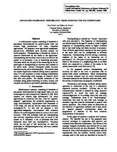
and Percentiles ���������������������������������������������������������������������Statistics ����������������� ��������������������������������������� ���������������� ���� ���� ��� �� ���� ���� ���� ���� ���� ���� ���� ���� �� ���� ���� ���� ���� ���� ���� ���� ��� �� ���� ���� ���� ���� ���� ���� ���� ��� �� ���� ���� ���� ���� ���� ���� ���� ����� ���� ���� ���� ���� ���� ���� ���� ���� ��� �� ���� ���� ���� ���� ���� ���� � �� � Mean Standard Deviation Median 1% 5% 25% 75% 95% 99% � � � � � � � � ������������������������������������������������������������������������������������������������������������������������������������������������������������������������� ��� � � � � � � � � � 1.789 1.810 4.000 1.000 2.000 3.000 5.000 6.000 9.000 ���������������������������������������������������������������������������������������������������������������������������������������������������������������������������
Figure 1. Distribution of lengths of contiguous packet trains to the same destination for Outgoing traffic
��
�
�
--
--
-6-
� �
�� �
�� �
�� �
�� �
��
�� �
�� �
�� �
��
100000
�
Number That Length
50000
� �� � � �� � � �� � ��� �
� �
-0
��
� � � � � � � � � � � � � � � � � � � � � � � � � � � � � � � � � � � � � � � � � � � � � � � � � � � � � � � � � � � � � � � � � � � � � � �
-0
50
100 Packet Train Length (Inbound)
150
�� ��������������������������������������������������������������������������������������������������������������������������������������������������������������������������� �
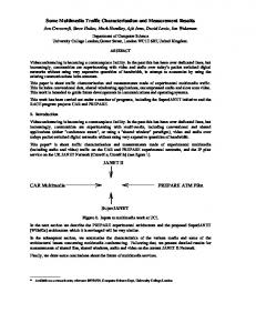
Statistics and Percentiles �� �������������������������������������������������������������������� � ���������������� ���� ���� �� ���� ���� ���� ���� ���� ���� ���� ��� �� ���� ���� ���� ���� ���� ���� ���� ��� �� ���� ���� ���� ���� ���� ���� ���� ��� �� ���� ���� ���� ���� ���� ���� ���� ���� �� ���� ���� ���� ���� ���� ���� ���� ��� �� ���� ���� ���� ���� ���� ���� ���� � ��������������������������������������� ���������������� � �� � �� � Mean Standard Deviation Median 1% 5% 25% 75% 95% 99% � � � � � � � � ����������������������������������������������������������������������������������������������������������������������������������������������������������� ��� ���������������� � � � � � � � � 2.383 3.393 4.000 1.000 2.000 3.000 5.000 7.000 16.000 � ���������������������������������������������������������������������������������������������������������������������������������������������������������������������������
� � ��
Figure 2. Distribution of lengths of contiguous packet trains to the same destination for Incoming traffic
As can be seen from these graphs, there are a large number of contiguous packet trains visible in the graphs. This is in part due to inadequate separation of the packets into incoming and outgoing streams, but is also evidence for burstiness of the data emerging from the network, especially considering the number of concurrent connections. These phenomena require further study, to determine whether the dynamics of the flow control mechanisms described by Clark et al,(8) such as "Ack Compression", are responsible for the packet bursts seen. In the sample, retransmits of TCP data packets were as follows:
�� �������������������������������������������������������� Packets 938345 �� ��������Total ������������������������������������������������ � � Total Rtxs 26534 � � ���������������������������������������� � ��������������� Syns 2294 �� ����Retransmitted ���������������������������������������������������� � � Out of Order Packets 35914 � �������������������������������������������������������
� � � � � �
The following graph shows the number of outbound and inbound packets during the time period.
--
--
-7-
�
5000
�� �� � ��� � � � � �� � � � � � � � �� � �� � � �� �� � �� � � ��� �� � � �� ��� � � ��� �� �� �� � � � � � � � �� � � � �� �� �� �� �� � �� �� � �� � �� � �� � �� �� �� � � �� � �� � � � � �� � � � � � � �� �� � �� � � � � �� � �� � � �� � � � � �� � �� � � �� �� � � �� �� � �� � � � � � �� �� � � � � � �� � � � � �� � � � � � � � � � � � � � � � � � � � � � �� �� � � �� � � � � � �� �� � � � � � � � � � � �� � � �� � � � �� �� �� � � � � ��� � � �� �� � � � �� �� �� � � � � �� � �� �� � �� �� � � �� �� � �� �� �� � � � �� �� � � � �� �� � � ��� � �� � � �� �� � � � �� �� �� � � � � �� � �� �� � �� �� � � �� �� � �� �� �� � � � �� �� � � �� � � � � � � � � � � � � � � � � � � � � � � � � � � � � � �� � � � �� �� � � � � �� �� � � � � � � � � � � �� � � �� � � � �� �� �� � � � �� �� � � �� �� � � � �� �� �� � � � � �� � �� �� � �� �� � � �� �� � �� �� �� � � � �� �� � � �
� �
4000 Outbound Pkts/min
3000
�
� �
� �
2000 1000
�
�
-0
��
�
�
� �� � ���� �� � � �� � �� �� �� �� � � � �� � �� �� �� �� � ���� �� �� � � �� � �� �� �� �� � � �� � � � � � �� ��� � � � � � �� � � ���� � � ��� �� � �� ���� � �� ��� ��� � �� ������ ���� �� � � �� �� � �� �� � � � � � � � �� �� � � �� �� �� �� � �� � ��� � � �� � � � �� � �� �� �� �� �� � � �� � �� � � � � � �� � � � � � � � � � � � � � � � �� � � � � �� �� � � � � � � � � �� �� � � � � � � � � �� �� �� �� �� �� �� � � � � � � �� � � �� � �� ��� �� ������� � �� �� � �� �� � � � � �� �� � � �� � � � �� � � � �� � �� � � �� ����� � � � �� � � � �� � � � � �� � �� �� � � �� � � � �� � � � � � � � � � �� � � � � � � � � �� � � �� � � � � �� � � � �� � � � � �� � � � � �� �� � � �� � � �� �� � � � �� �� � �� �� � � �� � �� � �� �� �� �� �� �� �� � �� � � � �� � �� ����� ���� �� � �� � �� ���� � � � �� � � � �� �� � � �� � � �� � � � �� �� �� � �� � �� �� �� � � �� � � � � � � � � �� �� � � � �� �� � � � � � � �� � � �� � � � � �� �� � � � � � � � �� �� � � � � � � � � � � � � � � � � � � � � � � � � � �� � � �� � � � �� �� � � � � � � �� � � � � �� �� � � � � � � � � � � � � � �� �� �� � ����� � ��� � � �� � �� � � � � � � � � � � � � � � � � � � � � � � � � � � � � � � � � �� � � �� � � � � � � �� � � � � �� �� � � �� � � � � � � � � �� � � � � � � � � �� � � �� � � � � � � � � � � �� � � � � � � �� � � � � � � � � � � � � � � � � � � � � � � � � � �� � � � � � � � � � � � � � � � � � � � � � � � � � � � � � � � � � � � � � � � � � � � � � � � � � � � � � � � � � � � � � � � � � � � � � � � � � � � � � � � � � � � � � � � � � � � � � � � � � � � � � � � � � � � � � � � � � � � � � � � � � � � � � � � � � � � � � � � � � � � � � � � � � � � � � � � � � � � � � � � � � � � � � � � � � � � � � �� � �� � � � �� � � � � � � � �� � �� �� � � � � � � � � �� � � � � � � � � � � � � � � � � � � � � � � � � � � � � � � � � � � � �� � � � � � � �� �� � � � � � � �� � � � � � � � � � � � � � �� � � � � � � � � � � �� � � � � � � � � � � �� � �� � � � � � � � � � � � � � � � � � � � � � � � � �� � � � � � � � �� � � � � � � � � � � � � � � � � � � � �� � � � � � � � � � � � � � � � � � � � � � � � � � �� � � � � � � ������������� �������� � ������� �� �� ��� ������� ��� �� ������������ � � ����� � ��������������� �� �������� ���� �������� � ���������� � �� �� �� � � �� � �������������� ������� �������� � � ������������������� ��������������� ��� � � � � � � � � � � � � � � � � � � � � � � � � � � � � � � � � � � �� � � � � � � � � � � � � � � � � � �� � � � �� � � � � � � � � � � � � � � � � � � � � � � � � � � � � � � � � � � � � � � � � � � � � � � � � � � � � � � � � � �� � � � � � � � � � � � � � �� � � � � � � � � � � � � � � � � � � � � � � � � � � � � � � � � � � � � � � � � � � � � � � � � � � � � � � � � � � � � � � � �� � � �� � � � �� � � � �� � � �� �� � � � �� �� � � � �� � �� � � � � �� �� �� �� �� � � � � � �� �� � � � � �� � � � � � � � � �� � � � � � � � � � � �� � � � � � �� � � � �� � � �� � � � �� � � � � � �� �� � � � � � � � �� � � � � �� �� � � � �� � �� � � � � � � � �� � � �� � � � � � �� �� � � �� � � � � � � � �� � � � � �� � �� � � �� � � � � � � � � � � � � �� � � � � �� � �� � � � � � � � �� � � � � � � � � � � � � �� �� � � �� � � � � � � � � � � � � � � � � � �� � � � �� � � � � � � � �� � � � � � � �� �� �� � � � � � � � �� � � �� � � � ��� � � � � � � � �� �� � � � � ��� � � � � � � � � �� � ��� �� ����� ���� � ����� � � �� �� ����� ��� �� ���� � �� ��� � ��� � ��� � � � ��� ������� � ����������������������������������������������������������������� �����������������������������������������������������������������������������������������������������������������������������������������������������������������������������������������
� � � � � � � � � � � � � � � � � � � � � � � � � � � � � � � � � � � � � � � � � � � � � � � � � � � � � � � � � � � � � � � � � � � � � � �
11.00gmt
12.00gmt
13.00gmt 14.00gmt Time (mins) from 10.49am
15.00gmt
16.00gmt
���������������������������������������������������������� � �����������������������Statistics ����������������������� �� ���� ���� ���� ���� ���� ���� ���� ���� ���� ���� ���� ���� ���� ���� ���� ���� ���� � Mean Standard Deviation � ������������������������� ����������������������������������� 2141.729 890.631 ���������������������������������������������������������
� � ��
Figure 3. Packet Rates for outgoing data over time � �
3000
��
� �
� � �� � � � �� � �� � �� �� �� � � � � �� � �� � � �� � �� � � �� ��� � � � � �� � �� � � � � � �� � � � �� �� �� � � �� � �� � �� �� �� �� � � � � � � �� � � � � � �� � �� �� � � � � �� � �� � � � � � �� ��� � � � � � �� �� � � ��� �� �� � �� � �� � � �� � �� �� � � �� �� ��� ��� �� � �� � � � ����� ��������������������� ���� � � � �� �� � � � � � � � � � � � � � � � � � � � � � � �� � � � �� �� � �� �� �� �� �� � � �� �� � �� �� �� �� �� �� � � � � �� �� �� � � � � � ���� � �� � � � �� �� � �� �� �� �� �� � � �� �� � �� �� �� �� �� �� � � � � �� �� �� � � � � � � � � � � � �� � � � � � � � � � � � � � � � � � � � �� � � � � � � � � � �
2000 �
Inbound Pkts/min � � �
1000 �
� �
-0
��
��
�� � �� � � � � � �� � � �� � �� �� � � �� �� � �� � � � ��� � �� � �� � �� �� � � � � � �� �� � � �� � � � � �� � ������ �� ����� �� � � � � ������� � � � � � � � � �� � � � �� � � � � � � � ��������� � � � � � � � � � � � �� � � � �� �� �� �� � � � � � � ���� �� �� � ���� � � � ��� � � � � � � � � � � �� � � � �� �� �� �� � � � � � ��� �� � � � �� � � � �� � �� � � � �� � � �� � �� �� �� � � � � � � � � �� �� �� �� �� � � �� � � � � �� �� �� �� � � � �� �� �� � � �� �� � �� � � � � �� �� � � � �� �� �� � � �� � �� �� � � � �� � �� ���� ��� �� ��� � � � � � � � � � � � � � � � � � � � � � � � � � � �� � � � � � �� � � �� � � � �� �� �� �� �� ��� � � � � � � � �� � � � � � � �� � � � � � � � � �� �� �� �� �� � � � �� �� �� � �� � � �� �� � � � � � � ��� �� �� � �� � � �� � � �� � �� � �� � � ��� � �� � � � � �� � �� �� � � � � �� �� �� � � � �� �� � � � � � � �� � �� �� � � � � �� �� � � � �� �� � � � � � �� � � �� �� �� �� �� � � � � � �� � � � �� �� � � �� �� �� �� �� � �� �� �� � � �� �� �� � � � � �� �� �� � � �� � � �� � � � � � � � � � � � � � � � � � � � � � � � � � � � � � � � � � � � � � � � �� �� � � � � �� � � � �� � �� �� ������� �� �� � � �� � � � �� � � � � �� � � �� �� �� �� �� � � � �� �� � � � � �� �� �� � �� �� �� �� �� �� � �� �� �� � � � �� �� �� �� �� �� � �� � �� �� �� �� �� � � � �� � � �� � � �� � �� � �� �� �� �� � �� � � �� � �� �� �� �� � �� � �� �� �� � �� � �� � � � �� �� � �� �� �� � �� � �� �� �� � � � �� �� �� �� � �� �� �� � �� � � � � � �� �� �� �� �� �� �� �� �� � �� �� � �� �� � � �� � � � � �� �� � �� �� � � � �� � � � �� �� �� �� �� � �� �� �� � � � � �� �� � � �� � � �� �� �� �� �� � � � � �� � �� �� �� � �� �� � � � � � � � � �� � � � � � �� �� �� � � �� � �� �� �� � � � � � � �� �� � � �� � � � � � � � � �� � � �� ��� �� �� � � � �� � � � � �� � � � �� �� � �� � � � � �� � � � �� � � � � � �� � � � �� �� �� � � � � � � � �� �� �� � � � �� �� �� �� � � � �� � �� � �� �� � � � � �� �� � � �� � � � �� �� � � � �� � �� � � �� � � � � � �� � �� � � �� � �� �� �� �� �� �� � � � �� � � � � �� � � � � �� � � � � �� � � � � � � � � � � � � � � � � � � � � � � � � � � � � � � � � � � �� � � � �� � � �� � �� � � � � � � � � � � � � � � � � � � �� � � � � � � � � � � � � � � � � � � � � � � � � � � � � � � � � � � � � � � � � � � � � � � � � � � � � � � � � � � � � � � � � � � � � �� � � � � � � � � � � � � � � � � � � � � � � � � � � � � � � � � � � � � � � � � � � � � � � � � � � � � � �� � � � ��� � � � �� � �� � � � � �� � � � � ���� � � �� � �� � � � � �� � � �� �� �� �� �� � �� �� � �� �� �� � � � � �� �� �� �� �� � �� �� �� �� � �� �� �� � � �� � � �� �� �� �� �� �� �� � �� �� � �� �� �� �� �� � �� �� �� �� � � �� � �� �� �� � �� � � �� � �� � �� �� �� �� � �� � �� �� � �� �� �� �� �� � �� �� �� �� �� �� � �� �� �� �� �� � �� �� �� � �� �� �� � �� �� � �� �� �� �� � �� �� �� � �� � � �� � � � � �� �� �� �� �� �� �� �� �� � �� �� � �� �� � � � � � � �� � � � �� �� � �� �� �� �� �� �� �� � �� �� �� �� �� � �� �� �� � �� � �� �� �� � � � �� � �� � �� � � �� � � �� �� �� �� �� �� � � �� � �� �� �� � �� �� �� �� �� �� � � � � � � � � � � � � � � � � � � � � � � � � � � � � � � � � � � � � � � � � � �� � � �� � � � � � � � � � � � � � � � � � � � � � � � � � � � � � � � �� � � � � � � � � � � � �� � � � � � � � � � � � � � � � � � � � � � � � � � �� � � � � �� � � � � � � � � �� � � � � � �� � � � � � � � � �� �� �� � �� � � � � � � � � � �� � � � � � � � � � � � � � � �� � � � � � � � � � � � � � � � � � � � � � � � � � � � � � � � � � � � � � � � � � � �� � � � �� � � � �� � � �� � � � � � � � � � � � � � � � � � � � � � � � � � � �
� � � � � � � � � � � � � � � � � � � � � � � � � � � � � � � � � � � � � � � � � � � � � � � � � � � � � � � � � � � � � � � � � � � � � � �
11.00gmt
12.00gmt
13.00gmt 14.00gmt Time (mins) from 10.49am
15.00gmt
16.00gmt
���������������������������������������������������������� � �����������������������Statistics ���� ���� ���� ���� ���� ���� ���� ���� ���� ���� ���� ���� ���� ���� ���� ���� ���� � ����������������������� �� � � Mean Standard Deviation ������������������������ ����������������������������������� � � � � 1215.062 506.683 ���������������������������������������������������������
Figure 4. Packet Rates for incoming data over time A brief period at around 11.30 can be seen when some networks became unavailable, with another period of outage in the same networks at 12.40. The distribution of packet sizes for both inbound and outbound packets can be seen below.
--
--
-8-
� �
� �
�� �
�� �
�� �
��
300000
�� �
�� �
�� �
��
200000
�
Number 100000 �
��
�
�
��
�
�
��
-0
��
�
�
� � � � � � � � � � � � � � � � � � � � � � � � � � � � � � � � � � � � � � � � � � � � � � � � � � � � � � � � � � � � � � � � � � � � � � �
0
100
200
300 400 512 600 700 800 Inbound: pktsize (bytes) v. #pkts that size
900
1024
���������������������������������������������������������������������������������������������������������������������������������������������������������������������������� �
Statistics and Percentiles ��������������������������������������������������������������������� ������������������� ������������������������������������� ���������������� ���� ��� �� ���� ���� ���� ���� ���� ���� ���� �� ���� ���� ���� ���� ���� ���� ��� �� ���� ���� ���� ���� ���� ���� ���� ��� �� ���� ���� ���� ���� ���� ���� ���� ���� ��� �� ���� ���� ���� ���� ���� ���� ���� ���� ���� �� ���� ���� ���� ���� ���� ���� ���� � �� � �� � Mean Standard Deviation Median 1% 5% 25% 75% 95% 99% � � � � � � � � ����������������������������������������������������������������������������������� ��������������������� ������������������������������������� ������������������� ���������������� � � � � � 353.236 231.971 512.000 0.000 1.000 30.000 521.000 536.000 747.000 ���������������������������������������������������������������������������������������������������������������������������������������������������������������������������
� � ��
Figure 5. Inbound packets - distribution of packet sizes
� �
� �
�� �
�� �
�� �
�� �
��
300000
�� �
�� �
�� �
�� �
�� �
��
200000
�
Number 100000
-0
� �
��
�
�
�
� � � � � � � � � � � � � � � � � � � � � � � � � � � � � � � � � � � � � � � � � � � � � � � � � � � � � � � � � � � � � � � � � � � � � � �
0
100
200
300 400 512 600 700 800 Outbound: pktsize (bytes) v. #pkts that size
900
1024
�� ��������������������������������������������������������������������������������������������������������������������������������������������������������������������������� �
Statistics Percentiles �� �������������������������������������������������������������������� ���� ��� �� ���� ���� ���� ���� ��and ���� ���� ��� �� �� ���� ���� ���� ���� ���� ���� ��� �� ���� ���� ���� ���� ���� ���� ���� �� ���� ���� ���� ���� ���� ���� ��� �� ���� ���� ���� ���� ���� ���� ���� ���� ���� ��� �� ���� ���� ���� ���� ���� ���� ���� ���� � � ����������������� ��������������������������������������� ���������������� �� �� � �� � Mean � Standard Deviation Median 1% 5% 25% 75% 95% 99% � ��������������� ��������������������� ����������������� �� ����������������� ��������������������������������������� ������������������� ����������������� ����������������� ���������������� � � � � � � � � � �� 74.971 175.196 3.000 0.000 1.000 2.000 6.000 512.000 521.000 � ��������������������������������������������������������������������������������������������������������������������������������������������������������������������������� Figure 6. Outbound packets - distribution of packet sizes
The different distributions of packet sizes for inbound and outbound traffic show the simplex nature of the data flow within the pipe, where most outbound traffic is acknowledgement of incoming data. When the packet size results shown above are combined with the packet rates, the average utilisation rates for inbound and outbound traffic 384 KBit/s link (adding a constant 40 bytes for TCP and IP headers):
������������������������ ����������������������������������������������������� ��������������������������������������� Average Utilisation (KBit/s) percentage utilisation �����Direction ������������������� ����������������������������������������������������� ��������������������������������������� � Outbound � � 32.83 8.5% ��������������������� ����������������������������������������������������� ��������������������������������������� ��� � � � Inbound 63.71 16.6% �����������������������������������������������������������������������������������������������������������������
� � � ��
The following graph how the number of TCP retransmissions and misordering of packets varied over the day.
--
--
-9-
� �
200
��
� �
150 �
� �
100 �
� �
50 �
� ��
-0
��
� ��
�
� � � �� � �� � �� ���� ��� �� � �� � � � � � �� � �� � � � � � � � � � � �� � � � �� �� � ������� � �� � � � �� � � � � � � � � � � � � � � � � �� �� � � �� �� � ���� � � � � � � � � �� � � � � � � �� �� � � � � � � � � � � �� � � �� � � � �� � �� � �� � � � � �� � � �� � � � �� � � � � � �� � � � � �� �� � � �� � � � � � �� �� � �� �� � � � � � �� � � �� �� �� �� �� �� � �� � �� �� �� � �� �� � �� � � � �� � � � � � � � � �� � �� � � � � � � � � � � � � � � � � � � � � � � � � � � �� � �� � � � � � � � �� �� � � �� � � �� � � � � � � �� � � � � �� � � � �� � � � � � � � � � � � � � �� � � � �� �� � � � � � �� � � � � � �� � �� � � � � � � � � � � � � � � � �� � � � � � � � � � � � � � � � � �� � � �� �� � �� �� � � � � � � � � � � � � �� � �� �� � � � � � � �� � �� � �� �� � � � � � � � � � � �� � � � � � � � � � � � � � � � �� � � � � �� � � � � � �� � � � � � � � �� � �� � � � �� �� �� � � � � � �� � �� � � �� �� ��� � � � �� � � �� � � �� � � � � �� �� �� �� �� �� �� � � �� �� � �� � �� � �� �� � � � � � � � � �� � �� � �� � � � �� � �� � �� � � �� � � �� �� � �� �� �� �� �� � � � �� �� �� � � � � � �� �� �� � �� � � � �� � � �� � � � � � � � � � � � �� �� � �� � � � � � �� � � � � � �� � � � �� � � � � � � � � � � � � � � � � �� � � � � � � � �� � � �� � � �� � � � �� � � � � � �� � �� � � � � ��
�
Inbound Retransmissions
�
��
��
��
��
�� �� �� ���� �� �� �� �� �� �� � �� � � �� � � � � � � �� � � � ����� �� �� � � �� �� ��� �� �� � � � � �� � � � �� � � � � � �� � � �� � � �� �� � � � �� � � � � � � � � � � � � � � �� � �� � � � �� � �� � �� � � �� � � � � � � � � � � � � � � � � � � � � � � � � � � �� � � �� �� � �� � � � � ��� � � � � � �� � � � � � � � � � � � �� �� �� � � ����� � �� �� �� ��� � � � � � � � � � � � �� � � �� � � � � �� �� � � � � �� � � � � � � � � � � � � � � � � �� � � �� � � �� �� ������ � � � � �� �� � � � � � � � � � �� � � � � � � � � � �� � � � � � � � � � �� � � � � � � � � � � � � � � � � � � �� � � � � � � � � � � � � � �� �� �� � � � � �� � � � � � � � � �� � �� � � �� � �� � �� � � � � � � � �� � � � �� � � �� �� � � � � � �� �� � �� � � � � � � � � � � �� � �� �� � � � � � � � � � � � �� �� � �� � � � �� � � � �� �� � � �� �� � � �� � �� � � � � � � �� � � �� � � � � �� � � � � � � � � �� � �� �� �� � � � � � � �� � � � � � �� �� � � �� � �� � � �� � � � � � � � � �� � �� � �� �� � �� � � �� �� � �� �� � � � � � � � �� �� �� � �� � �� � � � � � � �� �� ��� � �� � � �� �� � � �� � � � �� �� �� �� � �� � � �� �� �� � � � � � � � � � �� � �� �� � � � � � �� �� � �� � � � � �� �� �� � �� �� �� �� � �� �� � � �� � �� � � �� � � � �� � � � �� � � � �� � �� �� � � �� � �� � � �� �� �� � �� �� � � �� �� �� �� �� � � � �� � � �� � � �� � � � � � � � � � � � � � �� � � � � � � � � � � � � � � � � � � � � � � � � � � � � � � � � � � � � � � � � � � � � � � � � � � � � � � � � � � � � � � � � � � � � � � � � � � � � � � � � � � � � � �� �� � �� � �� �� � � � �� �� �� �� � �� �� �� � � � �� � �� � �� � � � � �� � � � �� �� �� �� � �� �� � � �� � � � � �� � � �� �� � � �� �� � �� � �� � � � �� � � �� � � � �� � � �� �� �� � � �� �� �� � � � � �� � � � � � � � � �� �� �� � �� � �� � � � �� � �� � � � � � � � �� � � �� �� �� � �� � � �� � � � � � �� �� � � �� �� � �� � � � � �� �� � � �� �� � � �� �� �� �� �� � � �� �� � � �� �� � � � � � � � � � �� � � � � � �� �� � � � � � � � � �� � �� � � �� � � � � � � � � � � �� �� � � � � � � � � � � �� � � � �� � � � �� � � � �� � � � � � � � � �� � � � � � � � �� � � � � � � � � � �� � � � � � � �� �� � �� � � � �� �� � �� � � � � � �� � � � �� � �� � � � � � � � � � � �� � � � � � � � �� �� � �� � �� � � � � � � �� � � � � �� � � � � � � � �� � � � �� � � � � � � � �� �� � � ��
��
�� � � �� � �� �� � �� � � � � � �� � � � � � � � �� � �� � �� � � � � � � � � � � � �� � �� �� � � � � �� �� �� � � �� � � � � � � �� � � ���� � ���� �� ��� ���� ������� ����� ���� ��������������� ���� �� ��� �� � ���� � ���� �� ���� ������������ ����� �� ��������������������� ������� ��� �� � � ����������������������
��
�� ��
� � � � � � � � � � � � � � � � � � � � � � � � � � � � � � � � � � � � � � � � � � � � � � � � � � � � � � � � � � � � � � � � � � � � � � �
11.00gmt
12.00gmt
13.00gmt 14.00gmt Time (mins) from 10.49gmt
������������������������������������������������������ ���������������������Statistics ������������������� ���� ���� ���� ���� ���� ���� ���� ���� ���� ���� ���� ���� ���� ���� ���� ���� ���� � Mean Standard Deviation � ��������������������� ����������������������������������� 79.952 41.978 �����������������������������������������������������
15.00gmt
16.00gmt
� � � ��
Figure 7. Retransmission Rates for incoming data over time �
�� �
��
� � �
40 Outbound Retransmissions
�
�� �� �� �� � �� � � � � � � �� � � � � � � � � �� � � � �� � � � �� �� �� � �� � � � � �� � �� � �� � � � � � � �� �� �� �� � �� � � � �� � �� � � � � � � � � �� � �� � � �� �� � � � � � � � � � � � �� � � � � � ��� � ��� ����� ��������� ���� � ����� � �� � � � � � � � � � � � � � � � � � � � � � � � � � � � �� � � � � � � ������ ������ ������������������ ������������������� � �
20
� �
�
� �
-0
��
�� �� ��
�� � �� � � �� � �� � � � � � �� �� � � � �� ������� �� �� �� � ��� ��������
��
��
�� ���� ���� �� ��� �� ����� �� �� ��� �� �� � �� � �� �� � � � � � � � � � � � � � � �� ���� �� �� ��� � � � � � �� �� � � � � �� �� � � � � � � � � � � � � �� � � �� � � � � �� � �� � � � �� � � � �� � � � � � �� � � � � � � � �� � � �
��
�� �� �� � �� � � � � �� � � � � � � � �� �� � � � � � � �� � � � � � � � �� � � � � � � � �� � � �� � � � � � � ��
�� � �� � �� �� � �� � � � � �� � �� � � � �� ��� �� �� �� �� ��� � � � �� � �� � � � � � � � � � � �� � � � �� � � �� �� � � �� � � � � � � � � � � � � � � � � � �� � � � � � � � � � � � � � � � � � �� � � � � � � � � � � � � � � � � �� � � � � � �� � � � � � � � � � � � � � � � � � � � � �� � � � � � � �� � � ��
�� �� ���� �� � � �� � � � ������ �� �� ��� ��� � � � ��� �� �� � ������� ��� ��
� � � �� � � � � �� � �� � �� � � � � � �� �� �� � �� � � � � � � � � � � � � �� � �� � � � � � � � � � � � � � �� � �
� �� � � �� � � �� � �� � ��� �� � � � �� � ����� � �� �� �� �� � � �� �� �� � � � �� �� �� � � � �� �� �� � �� �� �� �� � �� � � �� �
� �� ��
�� ��� �� �� �� � �� �� � � � � � � � � �� � �� �� � �� � � � � � �� � � � �� �� � � �� �� � � � �� � � � � �� � � � � � � � �
� � � ��� �� �� � � � �� � � � � � �� � � �� � �� � � � �� �� � � �� � �� � �� �� � � � � �� �� � � � � � �� � � � �� � �� � � �� � � �� � � � � � � �� � � � � � � ����� � � � � � �� � � � � � �� � � � � � � �� �� � � � � � � � �� � � �� � �� � �� �� � � �� � � � � � �� �� �� �
� � � � � � � � � � � � � � � � � � � � � � � � � � � � � � � � � � � � � � � � � � � � � � � � � � � � � � � � � � � � � � � � � � � � � � �
11.00gmt
12.00gmt
13.00gmt 14.00gmt Time (mins) from 10.49gmt
15.00gmt
������������������������������������������������������ � ���������������������Statistics ���� ���� ���� ���� ���� ���� ���� ���� ���� ���� ���� ���� ���� ���� ���� ���� � ������������������� ���� � Mean � Standard Deviation �������������������� ����������������������������������� � � � � 10.740 8.053 �����������������������������������������������������
Figure 8. Retransmission Rates for outgoing data over time A periodic pattern can be seen in the incoming packet stream. It is hoped that the ongoing work on the dynamics of flow control mechanisms will help in understanding this phenomenon, and reduce the fluctuations that are exhibited.
16.00gmt
--
--
- 10 -
� �
�� �
�� �
�� �
�� �
��
10000
Number That Time
�� �
�� �
�� �
��
5000
�
� �� � � �� �� �� � � �� �� �� � ����� � � �
-0
��
� � � � � � � � � � � � � � � � � � � � � � � � � � � � � � � � � � � � � � � � � � � � � � � � � � � � � � � � � � � � � � � � � � � � � � �
-0
50 100 150 Retransmitted Packet Inter Arrival Time Distribution (secs)
200
�� �������������������������������������������������������������������������������������������������������������������������������������������������������������������������� �
Statistics and Percentiles �� ������������������������������������������������������������������� � ���������������� ��������������������������������������� ���������������� ���� ���� ��� �� ���� ���� ���� ���� ���� ���� ���� ��� �� ���� ���� ���� ���� ���� ���� ���� ��� �� ���� ���� ���� ���� ���� ���� ���� ��� �� ���� ���� ���� ���� ���� ���� ���� ��� �� ���� ���� ���� ���� ���� ���� ���� ���� ��� �� ���� ���� ���� ���� ���� ���� ���� � Mean Standard Deviation Median 1% 5% 25% 75% 95% 99% � � � � � � � � ��� ���������������� ��������������������������������������� ��������������������� ����������������� ����������������� ����������������� ����������������� ������������������� ��������������� 17.649 614.654 0.900 0.000 0.100 0.300 3.500 74.900 75.500 � ��������������������������������������������������������������������������������������������������������������������������������������������������������������������������
� � ��
Figure 9. Time interval between retransmissions of same packet
The high number of retransmissions and especially the retransmitted SYN packets shown here was surprising. However upon closer examination the problem was shown to be an old version of TCP software running on the VAX mail server (Ultrix 2.1A based on 4.2BSD), which used a fixed retransmission timer, set to 0.5 seconds, when the normal round trip time was between 0.3 to 1.0 seconds. Discussions with ULCC showed the reason for the old software was due to the need for Operating System stability, an understandable desire which should be appreciated by all those who propose radical shake-ups of operating networks and machines to integrate the latest "enhancement" to the overall system. Unfortunately the analysis was also unable to determine whether a packet was a retransmission or an out of order packet that filled a hole in the sequence space that was greater than the size of one packet. The majority of the low gap retransmissions are caused by out of order packets. What proportion of the retransmissions are really out of order packets is to a certain degree irrelevant. What is important in this data is there is obviously a large number of data packets that arrive out of order, due to whatever reason. It has been suggested for the "Slow Start" algorithm that any packet arrival should trigger the transmission of an ack packet, and if this ack packet does not advance the acknowledged sequence space, then the received ack should be used as a signal that a packet has been lost due to congestion, and should thus trigger the congestion recovery mechanisms. However, with upto 5% of all packets arriving out of order, this is likely to decrease the throughput efficiency of the TCP implementations unnecessarily, unless the out of order arrival of packets is due to congestion at the routers interfering with the FIFO queueing and transmission of packets. The observed peaks at 64 and 74 seconds are explained below.
--
--
- 11 -
�
��� � �� �� � � � �� � �� � � � � � � � � � � � � � � � � � �� � � � �� � � � �� �� � � � �� � � � � �� �� � � � � � � �� �� �� � �� �� �� � �� �� �� � � � � � �� � �� �� � � �� � � � � � �� � � � � � �� �� � �� � � � �� � � � � � � � � � � � � � �� � � � � � � � � � � � � � � � � � ���� �� � � � � �� � �� � � � � �� �� �� � � � � � �� �� � �� � �� � � � � �� �� �� � � � � � �� � �� � � �� � � �� �� � �� � � � � � � � � �� �� �� �� �� �� � � � �� � �� � � � � � � � � � �� �� � � � �� � �� �� �� � �� �� � �� � �� � � �� �� � �� � �� � � � � � � � � � � � � � � � � � � � � � � � � � �� �� � � �� � � �� � � � �� �� � � �� � � � � � � �� � � �� �� � � � � � � � � � � �� � �� � � � � � �� � � � � � � � �� � � � � � �� �� � �� � � � � � � � �� � �� � �� � � � � � � � � � � � �� � � � � � � �� � � � � � � � �� �� � �� � � � � � � �� � �� � � � � � � � � � � � � � � � � � � � � � � � � � � � � � � � � � � � � � � � � � � � � � � � � � � � � � � � � � �� ��� �� � � � � �� �� � � � � � � � �� � � � �� �� � �� �� �� ��� ��� � � � � �� � � �� �� � �� �� � � � �� �� �� �� �� � � �� � � � � �� � � � � � �� �� � �� �� �� �� � � �� �� �� �� �� � � �� � �� �� �� �� ��� �� �� �� �� �� � � � �� � � �� �� �� �� � � �� �� � �� �� � � � �� � � �� � �� �� �� � �� � � � �� � � �� �� � � � �� �� � � � � �� �� � �� � � � � � �� �� �� � �� � �� �� �� �� � �� �� � �� � �� � �� � � � � � �� � � � � � � � � � � � � ��� � � ��� � � � � � �� �� � � � � � � � � � � � �� � � � � � � � � � � � � � � � � � � � � � � � � � � � � � � � � � � � � � � � � � � � � � � � � � � � � � � � � � � � � � � � � � � � � � � � � � � � � � � � � � � � � � � � � � � � � �� � � � � � � � � � � � � � � � �� � � �� � � �� � � � � �� �� � �� � � � � � � � � � � �� �� �� � � � � � � � � �� �� � � � � � � �� �� �� � � � � � �� � �� � � � � � � � � � � � � � � �� �� � �� � � �� � � � � � � �� � �� � �� �� � � �� �� � � � � � �� �� �� � � � � � � � � � �� � � � � �� � �� � � � � � � � � � �� � �� � �� � � �� � �� � � � � � �� � �� � � � � � � � �� � � �� � � � � �� � � � �� � �� � � � � � � � � � � � � � � � � � �� �� � � � � �� � � � �� �� �� �� � � � �� � � � � ��� �� �� � � � �� �� �� �� � �� � �� �� �� � � � � �� �� � � � � �� � �� � �� � � � � �� �� � � �� � � � �� ��� � �� �� � � � �� � �� ��� �� �� � � �� �� �� �� �� � � ��� �� �� �� � � � � �� ��� �� � � �� � � �� �� �� �� � � � � �� �� � � � �� �� � � � � � �� �� � � �� �� � � � � � � � � �� � �� �� �� �� �� � �� � � � � � � � �� � � � � � � �� �� � � � � � �� � � � � � �� �� � �� � �� �� � �� � �� � � � �� �� �� �� �� � �� �� � � �� � �� � �� �� � �� � � � � �� � � �� � � � � � �� �� � �� �� � � � �� � � � �� �� � �� � �� �� � �� �� � � �� � � �� �� �� �� � �� � �� �� �� � �� � � � � � �� �� �� � �� �� �� � �� �� � � � � � � �� � �� �� � � �� � � � � � � � � � � � � � � � � � � � � � � � � � � � � � � � � � � � � � � � � � � � � �� � � � � � � � � � � � � � � � � � � � � � � � � � � � � � � � � � � � � � � � � � � � � � � � � � � � � � � � � � � � � � � � � � � � � � � � � ��� �� � �� � � � � �� � �� � � � � � � � �� �� �� � �� � � � �� �� � � � � � �� � � � � � � � � � � � � � � � �� � � � � � � �� � � � �� � � � �� � � �� � � � � �� � � � �� �� � � �� � � �� � � � � � � �� � � � � � � � �� � �� � �� � � � � �� �� � � � �� � � � � � � �� � � � � � � � � � � � � � �� � � �� � �� � � � � � � � � � � � � � � � � � �� � � � � � � � � � � � � � � � � � � � � � � �� � � � �� � � �� � � � �� � � �� � � � � �� � � � � � � �� � � �� � � � � � � �� � � � � � � � � � � � �� � �� � � � � � �� � � � � � � � �� � � � � � �� �� � �� � � � � � �� �� �� � �� � �� � � � � � � � � � �� � �� � � � � � � � � � � � � � � � � � � � � � � � � � � � � � � � � � � � � � � � � � � � � � � � � � � � � � � � � � � � � � � � � � �� � � � � � � � � � � � � � � � � � � � � � � � � � � � � � � � � � � � � � � � � � � � � � � � � � � � � � � � � � � � � � � � � � � � � � � � � � � � � � � � � � � � � � � � � � � � � � � � � � � � � � � � � � � � � � � � � � � � � � � � � � � � � � � � � � � � � � � � � � � � � � � � � � � � � � � � � � � � � � � � � � � � � � � � � � � � � � � � � � � � � � � � � � � � � � � � � � � � � � � � � � � � � � � � � � � � � � � � � � � � � � � � � � � � � � � � � � � � � � � � � � � � � � � � � � � � � � � � � � � � � � � � � � � � � � � � � � � � � � � � � � � � � � � � � � � � � � � � � � � � � � � � � � � � � � � � � � � � � � � � � � � � � � � � � � � � � � � � � � � � � � � � � � � � � � � � � � � � � � � � � � � � � � � � � � � � � � � � � � � �� �� � � � � � � � � � � � �� � � � � � � � � �� � � � � � � � � � � � � � � � � � � � � � � � � � � � � � � � � � � � � � � � � � � � � � � � � � � � � � � � � � � � � � � � � � � � � � � � � � � � � � � � � � � � � � � � � � � � � � � � � � � � � � � � � � � � � � � � � � � � � � � � � � � � � � � � � � � � � � � � � � � � � � � � � � � � � � � � � � � � � � � � � � � � � � � � � � � � � � � � � � � � � � � � � � � � � � � � � � � � � � � � � � � � � � � � � � � � � � � � � � � � � � � � � � �� � � � � � � �� � � � �� �� � � � � �� � � � � � � � � � � �� �� �� � � � � � � �� � � �� �� � �� � � �� � � �� � � �� � � � �� � �� � � � � � � � �� � � �� � �� �� �� � � � �� � � �� � � � �� � �� �� � � � � �� � � � � � � � � � � �� �� � �� � � �� � � � � � � �� � �� � �� �� � � �� �� � � � � � �� �� �� � � � � � � � � � �� � � � � �� � �� � � � � � � � � � �� � �� � �� � � �� � �� � � � � � �� � �� � � � � � � � �� � � �� � � � � �� � � � �� � �� � � � � � � � � � � � � � � � � � �� �� � � � � �� � � � �� �� �� �� � � � �� � � � �� �� �� ��� ��� � � �� �� � � � �� � �� �� � ��� � � � � �� �� � �� �� � � �� �� �� �� � ����� � � �� � �� � �� � � ����� �� � � �� � � � �� �� � �� � �� �� � ���� � ��� � � ��� �� �� � ���������������������������������������������������������������������������������������������������������������������������������������������������������������������������������������������������������������������������������������������������������������������������������������������� � �
200 � � �
150 Simultaneous Connections
� � �
100 � �
50 � � ��
-0
� � � � � � � � � � � � � � � � � � � � � � � � � � � � � � � � � � � � � � � � � � � � � � � � � � � � � � � � � � � � � � � � � � � � � � �
11.00gmt
12.00gmt
13.00gmt 14.00gmt Time (mins) from 10.49 am
�������������������������������������������������������� �����������������������Statistics ��������������������� ���� ���� ���� ���� ���� ���� ���� ���� ���� ���� ���� ���� ���� ���� ���� ���� ���� � Mean Standard Deviation � ����������������������� ����������������������������������� 130.603 40.770 �������������������������������������������������������
15.00gmt
16.00gmt
� � � ��
Figure 10. Number of concurrent connections over time The maximum number of connections here is surprisingly large - although one should note that FTP may account for two connections per user quite often. Informal discussion with ULCC indicated that as many as 40 FTPs go on at any one time from just one of the ULCC machines. The steady growth of the number of connections leads us to suspect that connections are not always terminated in a tidy manner, so that our experimental script cannot determine the correct termination of a connection. In particular, the rerouting of the networks observed above resulted in our analysis method failing to detect the termination of some of the observed connections. �
1500
Number of Connections
�
� �
�� �
�� �
��
�� �
�� �
�� �
��
1000
�
� �� � �
500
�� � � ��
�� �� �� � � �
-0
��
� � � � � � � � � � � � � � � � � � � � � � � � � � � � � � � � � � � � � � � � � � � � � � � � � � � � � � � � � � � � � � � � � � � � � � �
-0
5000 Time (secs)
10000
�� ��������������������������������������������������������������������������������������������������������������������������������������������������������������������������� �
Statistics Percentiles �� �������������������������������������������������������������������� ���� �� ���� ���� ���� ���� ��and ���� ��� �� ���� �� ���� ���� ���� ���� ���� ��� �� ���� ���� ���� ���� ���� ���� ��� �� ���� ���� ���� ���� ���� ���� ���� ���� ��� �� ���� ���� ���� ���� ���� ���� ���� ���� ��� �� ���� ���� ���� ���� ���� ���� ���� ���� ���� � � ����������������� ������������������������������������������������������� �� �� � �� � Mean � Standard Deviation Median 1% 5% 25% 75% 95% 99% � ��������������� ����������������� ��������������� ������������������� ������������������� ������������������� �� ����������������� ��������������������������������������������������������� � � � � � � � � � �� 83.196 415.369 9.000 0.000 1.000 2.000 26.000 368.000 1208.000 � ��������������������������������������������������������������������������������������������������������������������������������������������������������������������������� Figure 11. Connection duration for all connections over time
It is interesting to note that most connections have a short duration - the median duration is between 9 and 10 seconds, yet some connections will last almost 12000 seconds, thus leading to a large deviation in the statistic.
--
--
- 12 -
� �
� �
�� �
�� �
�� �
�� �
�� �� ��� � ��
�
�� �
�� �
�� �
�� �
�� �
1000
Number
500
� ��
-0
� � � � � � � � � � � � � � � � � � � � � � � � � � � � � � � � � � � � � � � � � � � � � � � � � � � � � � � � � � � � � � � � � � � � � � �
-0
5000 Data Pkts per Connection
10000
�� ��������������������������������������������������������������������������������������������������������������������������������������������������������������������������� �
Statistics and Percentiles �� �������������������������������������������������������������������� � ������������������ ���� ��� �� ���� ���� ���� ���� ���� ���� ��� �� ���� ���� ���� ���� ���� ���� ���� �� ���� ���� ���� ���� ���� ���� ���� ��� �� ���� ���� ���� ���� ���� ���� ���� ��� �� ���� ���� ���� ���� ���� ���� ���� ���� ���� �� ���� ���� ���� ���� ���� ���� ���� ���� � ������������������������������������� ���������������� � �� � �� � Mean Standard Deviation Median 1% 5% 25% 75% 95% 99% � � � � � � � � ��������������������������������������������������������������������������������������������������������������������������������������������������������� ��� ������������������ � � � � � � � � 101.132 410.333 28.000 6.000 7.000 10.000 45.000 367.000 1819.000 � ���������������������������������������������������������������������������������������������������������������������������������������������������������������������������
� � ��
Figure 12. Number of packets sent per connection - total
� �
�� �
�� �
��
�
�� �
�� �
��
1000
Number
� �� � � �� � � �� � � �� � � �� �� � � �� �� �� � �����
500
� � � � � �
-0
��
�� � �� �� �� ��� � �� � �� �� � � � �� � � �� �� � �
�� �� � � �� � � �
� � � � � � � � � � � � � � � � � � � � � � � � � � � � � � � � � � � � � � � � � � � � � � � � � � � � � � � � � � � � � � � � � � � � � � �
0
10
20
30
40 50 60 70 Data Pkts per Connection
80
90
100
Figure 13. Number of packets sent per connection - magnified As will be seen below, the large clump at around size 30 is due to SMTP connections. A large number of connections have only 7 packets transferred, consisting for example of ftp-data connections that transfer small files (less than 512 bytes) or the results of ’ls’ commands.
--
--
- 13 -
�
1e+06
� �
�� �
�� � � �� � � � � � � �� � � � � �� �� � � � � �� � � � � �� �� � � � �� � � � �� � � � � � � �� � � �� � � � � �� �� �� ��� �� � �� � �� �� � �� �� �� �� � � �� �� �� � � � � � �� � �� � �� �� � �� �� �� �� � � �� �� �� � � �� �� � � � � � � �� � � � � � � �� � � �� � � �� � � � � �� � � � �� �� � � � � � � � � �� �� �� �� �� ����� ���� � �� � �� � �� �� � �� �� �� �� � � �� �� �� � � �� �� � �� �� �� �� �� �� �� �� �� �� � � � � � � � � � � � � � �� � �� � � � �� � �� � �� �� � �� �� �� �� � � �� �� �� � � �� �� � �� �� �� �� �� �� �� �� �� �� � � � �� �� �� �� �� �� �� � � � � � � � � � � � � � � � � � � � � � � � � � � � � � � � � � � � � � � � �� � � � � � � � �� � � �� � � � � �
100000 10000
�
�
Number That Gap
1000
�
100
�
10
�
�
�
1
��
�
�
�
� � � � � � � � � � � � � � � � � � � � � � � � � � � � � � � � � � � � � � � � � � � � � � � � � � � � � � � � � � � � � � � � � � � � � � �
-0
1000 2000 3000 Inter Packet Distribution for all packets (msecs)
���������������������������������������������������������������������������������������������������������������������������������������������������������������������������� �
Statistics and Percentiles ��������������������������������������������������������������������� ����������������� ������������������������������������� ������������������ ����� ���� ���� ���� ���� ���� ���� ���� ���� ��� �� ���� ���� ���� ���� ���� ���� ���� ��� �� ���� ���� ���� ���� ���� ���� ���� ���� �� ���� ���� ���� ���� ���� ���� ���� ��� �� ���� ���� ���� ���� ���� ���� ���� ����� ���� ���� ���� ���� ���� ���� ���� ���� � �� � Mean Standard Deviation Median 1% 5% 25% 75% 95% 99% � � � � � � � � ������������������������������������������������������������������������������������������������������������������������������������������������������������������������� ��� � � � � � � � � � 21.051 29.120 40.000 10.000 20.000 30.000 50.000 70.000 130.000 ���������������������������������������������������������������������������������������������������������������������������������������������������������������������������
� � ��
Figure 14. Interpacket gap in time for all packets
This shows the measured probability distribution for the inter-arrival times between any two consecutive packets (from any source). As expected, due to the large statistical multiplexing involved in the data connections using the pipe, the distribution tends towards the expected exponential distribution. An anomaly can be seen at around 0.5 secs, probably due to probe packets sent out during the brief outage at 11.30. The following graphs show the interpacket gap for packets to the same destination, ie the gap between the same host appearing as destination for a packet.
--
--
- 14 -
�
100000 �
� �
���
�
��� �
���
10000
���
Number That Gap
��� ��� ��� � ���
1000
��� � ����� � ���
���� �
���
100
�� �
��� ���� �� �� �� ��� �� � �� �� ���
10
� � � ��
1
� � � � � � � � � � � � � � � � � � � � � � � � � � � � � � � � � � � � � � � � � � � � � � � � � � � � � � � � � � � � � � � � � � � � � � �
-0
100000 200000 300000 Inter Packet Gap Distribution (Outbound)
400000
500000
���������������������������������������������������������������������������������������������������������������������������������������������������������������������������� �
Statistics and Percentiles ��������������������������������������������������������������������� ������������������� ������������������������������������� ���������������� ���� ����� ���� ���� ���� ���� ���� ���� ���� ��� �� ���� ���� ���� ���� ���� ���� ��� �� ���� ���� ���� ���� ���� ���� ���� �� ���� ���� ���� ���� ���� ���� ���� ��� �� ���� ���� ���� ���� ���� ���� ���� ���� ����� ���� ���� ���� ���� ���� ���� ���� ���� ���� � �� � Mean Standard Deviation Median 1% 5% 25% 75% 95% 99% � � � � � � � � ������������������������������������������������������������������������������������������������������������������������������������������������������������������������� ��� � � � � � � � � � 543.310 8022.848 6.000 0.000 1.000 2.000 16.000 218.000 3346.000 ���������������������������������������������������������������������������������������������������������������������������������������������������������������������������
� � ��
Figure 15. Interpacket gap in packets for packets to the same outbound destination �
100000
�� � � �
10000 Number That Gap
� � � �
1000
� � � �
100
� � � � �
10 1
� � � � � ��
� �� �� � � �� �� �� � �� �� �� � �� �� �� �� �� � � �� �� �� � � �� �� �� � � �� �� �� � � �� �� �� � � �� �� �� � � �� �� �� � � �� �� ��
� �� � �� � �� � �� � �� � �� � �� � �� � �� � �� � �� � �� � �� � �� � �� � �� � �� � �� � �� � �� � �� � ��
�� � � � � � � � �� � �� �� �� � � �� �� � �� � � � �� �� � �� � � � �� �� � �� � � � �� �� � �� � � � �� �� � �� � � � �� �� � �� � � � �� �� � �� � � � �� �� � �� � � � � � � ��
��� �� �� �� � � �� � � �� � � �� � � �� � � �� � � �� � � �� � � �� � �
� �� � �� �� � � �� �� � � �� �� � � �� �� � � �� �� � � �� �� � � �� �� � � �� �� � � � ��
�� �� �� �� �� � �� �� � �� �� � �� �� � �� �� � �� �� � �� �� � �� �� �
���� � � �� �� � � �� �� � � �� �� � � �� �� � � �� �� � � �� �� � � �� �� ����
���� �� � � � �� �� � � �� �� �� � � �� �� �� � � �� �� �� � � �� �� �� � � �� �� �� � � �� �� � � � ��
�� �� �� � �� �� �� �� � � �� �� �� � � �� �� �� � � �� �� �� � � �� �� �� � � �� �� �� � � �� �� �� � �
�� � �� � �� � �� � �� � �� � �� � �� �
�� � �� �� �� �� �� �� �� �� �� �� �� �� �� �� �� �� �� �� �� �
� � � � �� �� �� �� �� � � �� �� �� �� � � �� �� �� �� � � �� �� �� �� � � �� �� �� �� � � �� �� �� �� � � �����
�� � �� � �� � �� � �� � �� � �� � �� � �� � �� � �� � �� � �� �� ��
�� �� �� �� �� �� �� �� �� �� �� �� �� �� �� �� �� �� �� �� ��
�� �� �� �� � �� �� � �� �� � �� �� � �� �� � �� �� � ��
�� � � � �� � �� � �� � �� � �� � ��
� �� � �� � �� � �� � �� � �� � ��
� ��� � � �� �� � � �� �� � � �� �� � � �� �� � � �� �� � ���
��� �� �� �� �� �� �� �� �� �� �� �� �� �� �� �� ���
��� �� �� �� �� �� �� �� �� �� �� �� �� �� �� �� ���
��� ��� ��� ��� ��� ��� ��� ��� ��� ��� ��� ���
���� �� � � � �� �� � � �� �� �� � � �� �� �� � � �� �� �� � � �� �� � � � ��
�� �� �� �� �� �� �� �� �� �� �� �� �� �� �� �� �� ��
� � �� ��� ��� ��� ��� ��� ��� ��� ��� ��� ��� ���
�� �� �� �� �� � �� �� � �� �� � �� �� � �� �� �
�� �� �� �� �� � �� �� � �� �� � �� �� � �� �� �
�� �� �� �� �� � �� �� � �� �� � �� �� � �� �� �
� ��� � ��� � ��� � ��� � ��� � ���
��� ��� ��� ��� ��� ���
� � � � � � � � � � � � � � � � � � � � � � � � � � � � � � � � � � � � � � � � � � � � � � � � � � � � � � � � � � � � � � � � � � � � � � �
-0
50 Inter Packet Gap Distribution (Outbound)
100
Figure 16. Interpacket gap in packets for packets to the same outbound destination - magnified The bar at -1 shows the total number of destinations that the packets have been seen. In examining the lower graph, it is possible to see two distinct linear regions, from a gap of 1 to around 25 and then out from 25. This would suggest that the distribution of packet gaps should be constructed from two distributions, to produce the linear regions shown. This phenomenon was used as the starting point for Jain to derive the Packet Train model of inter-arrival times for packet networks.(9) The packet train model of Jain is based on conversations between pairs of hosts. Each conversation is called a train, and each train between a pair of hosts is separated by a large temporal gap. In each train, the packet exchanges are broken into contiguous sequences of packets in one direction, called a trailer, followed by another sequence of packets in the opposite direction - the tandem trailer. The results of mapping the data onto this form of model are shown below4.
--
--
- 15 -
�������������������������������������������� ��������������������� ������������������������������������� ������������������������������������������� Parameter deviation of��Variation � ��standard � ��Coefficient ��������������� � ����mean ���������������� ���� ���� ���� ���� ���� ���� ���� ���� ���� ���� ���� ���� ���� ���� �������� ���� ���� ���� ���� ���� ���� ���� ������ ���� ���� ���� ���� ���� ���� ���� ���� ���� ���� ���� ���� ���� ���� ���� ���� ������ ���� ���� ���� ���� ���� ���� ���� ���� ���� ���� ������ ���� ���� ���� ���� ���� ���� ���� � � � � Inter-train gap (/s) 375.1 1332.0 3.55 �������������������������������������������� ��������������������� ������������������������������������� ������������������������������������������� Inter-trailer gap (/s) 0.203 0.524 2.57 ������� ������������������������������������� ��������������������� ������������������������������������� ������������������������������������������� � � � � Inter-car gap (/s) 0.167 0.472 2.83 �� � ����������������������������������������� ��������������������� ������������������������������������� ������������������������������������������� size (/packets) 1.872 1.299 0.69 �����Trailer ��������������������������������������� ���������������������� �������������������������������������� ������������������������������������������� � Train size (/packets) � 32.54 303.86 9.34 �� �� ���� ���� ���� ���� ���� ���� ���� ���� ���� ���� ���� ���� ���� ���� ���� ���� ���� ���� ���� ��� �� ���� ���� ���� ���� ���� ���� ���� ���� ���� ���� ���� ���� ���� ���� ���� ���� ���� ���� ���� ���� ���� ���� ���� ���� ���� ���� ���� ���� ���� ���� ���� ���� ���� ���� ���� ���� ���� ���� ���� ���� ���� ���� ���� ���� ���� ���� ���� ���� ���� ��� � � Total number of trains 30186 ��������������������������������������������������������������������������������������������������������������������������������������������� � � � � � � � � �
The results of Jain’s analysis are shown below.
��
�� ����������������������������������������� ��������������������� ������������������������������������� ������������������������������������������� deviation of��Variation �� ������������Parameter � ����mean � ��standard � ��Coefficient � �������������� ���� ���� ���� ���� ���� ���� ���� ���� ���� ���� ���� ���� ���� ���� �������� ���� ���� ���� ���� ���� ���� ���� ������ ���� ���� ���� ���� ���� ���� ���� ���� ���� ���� ���� ���� ���� ���� ���� ���� ������ ���� ���� ���� ���� ���� ���� ���� ���� ���� ���� ������ ���� ���� ���� ���� ���� ���� ���� � � � � Inter-train gap (/s) 23.773 118.86 5.0 �� ����������������������������������������� ��������������������� ������������������������������������� ������������������������������������������� gap (/s) 0.0652 �� ����Inter-trailer ������������������������������������� ��������������������� ������������������������������������� ������������������������������������������� � � � Inter-car gap (/s) 0.0342 � � � ����������������������������������������� ��������������������� ������������������������������������� ������������������������������������������� size (/packets) 1.8 �� ��Trailer ���������������������������������������� ���������������������� �������������������������������������� ������������������������������������������� �
Train size (/packets) 17.4 � �������������������������������������������������������������������������������������������������������������������������������������������
� � � � � � � � �
Jain’s data was taken from an analysis of a Local Area Network, whereas our data comes from measurements at the entry point to a stub network. This explains why the inter-trailer gaps and the intercar gaps are significantly larger. In addition, because our measurments are taken very close to the terminating machines of the conversations, the measurements of the inter-trailer times should have a bimodal distribution, with a fast response in one direction, and a slow response in the other, thus resulting in a higher Coefficient of Variation than would otherwise have been expected.
����������������������������������� 4. Coefficient of Variation is defined as the ration of standard deviation to mean.
--
--
- 16 -
� � � �
�� �
��
100000
� � � ���
10000 Number That Time
�� ��� � �� �� �
���
1000
�� �
��� ���� �
�� �� ��� ��� ��� ��� ���
100 10
�
�
�
1
��
�
� � � � � � � � � � � � � � � � � � � � � � � � � � � � � � � � � � � � � � � � � � � � � � � � � � � � � � � � � � � � � � � � � � � � � � �
-0
20000 40000 Outbound Inter Packet Arrival Time Distribution to same destination (secs)
60000
�� �������������������������������������������������������������������������������������������������������������������������������������������������������������������������� �
Statistics and Percentiles �� ������������������������������������������������������������������� � ������������������ ��������������������������������������� �������������� ���� ���� ���� ��� �� ���� ���� ���� ���� ���� ���� ���� ��� �� ���� ���� ���� ���� ���� ���� ���� ��� �� ���� ���� ���� ���� ���� ���� ���� ��� �� ���� ���� ���� ���� ���� ���� ���� ��� �� ���� ���� ���� ���� ���� ���� ���� ��� �� ���� ���� ���� ���� ���� ���� ���� � Mean Standard Deviation Median 1% 5% 25% 75% 95% 99% � � � � � � � � ��� ������������������ ��������������������������������������� ��������������������� ����������������� ����������������� ����������������� ����������������� ����������������� ��������������� 145.566 2431.541 0.150 0.000 0.050 0.100 0.200 4.900 80.400 � ��������������������������������������������������������������������������������������������������������������������������������������������������������������������������
� � ��
Figure 17. Interpacket gap in packets for seconds to the same outbound destination �
� �
��
100000 �
� � � �� � � ��� �� ���� � � � � �� � ���� � � � � � � � � � � �� � �� � � �� � ���� � �� � � � � � � � � �� � �� � � �� � � � � � �� �� � � � � � � � �� �� � �� � �� � � �� � � � � � � � � � � � �� � � �� � � � � � � � � � � � � � �� � � ��� �� �� �� � ��� �� � � � � �� ��� � �� � � � � � � �� � � �� � �� �� � � � �� �� �� � �� � � �� � �� � � �� � �� � � � ��� � �� � � �� � �� � � �� ��� � � � � � � � � �� � � � � � � � � � � �� � �� �� � � � �� � � � � � � � � � � � � � � � � � � ��� �� � � � � � � � � � � � � � � �� � � � � � �� � � �� � � � �� �� � �� � �� � � � �� � � � � � � �� � � � � � �� � � �� �� �� � � �� � � � � � � � � � � �� � � � � � � �� � � � � � � �� �� �� � �� � � � � � � � �� �� � �� �� � � �� � � � � � � �� � � � � � � � � � � � �� �� � � �� � � � � � � ��� �� �� �� � ��� �� � � � � �� ��� � �� � � � � � � �� � � �� � �� �� � � �� �� �� � � � �� � � �� � � � �� � � � � �� � � � �� � � �� � �� ��� � �� �� � � � �� �� ��� � � �� � � � � �� � ��� ��� �� � �� ��� � � � �� � � � � �� �� �� � �� � �� �� � �� � � � � � �� � � � �� � �� �� � � � � �� � � � �� ��� � � � �� �� � �� � � � �� � ��� � � � �� � �� �� �� � � � � � � � �� � � � � �� � �� � � � � �� �� �� � �� � � �� � �� �� � � � � �� � � � �� � � � ����� � �� � �� � � � � �� � � � �� � � � �� � �� � � �� � �� � � � �� � ���� � � � � � � � �� � � � � � � � �� ��� �� �� � � � � � � � � � � �� � �� ��� � � �� �� � �� � � � � �� � � � � � � � �� � � �� � � � � �� � � �� � ��� ��� � � �� � � � � �� � �� �� � � � � � � � �� � �� � � � �� � � �� �� � � � �� � �� � �� �� � � �� � �� �� � �� � � � � �� ��� � � �� � � � � � �� � � � � � � �� �� �� � � �� � �� � � � �� �� � �� �� � � �� � �� �� � � � � � � � � � � � �� � � �� � � � �� � � � ��� �� �� � � �� � � �� � � � � � � � �� �� �� � ��
10000
�
�
Number That Time
1000
�
�
100
�
�
10
�
�
�
1
��
�
� �� � � � � � � � � � � � � � � � � � � � � � �� � � �
�� � � � �� � � � � �� � �
� �
� �� �� � �� � � � �
�� � � � � � � � � � � � �� � � � � �� � �� � � � � �� � � � � � � �� � � � � � � �� � � � � �� � � � � � � �� �� �� �� � � �� � � �� �� � � �� � � � � � � � �� � � � � � � � � �� � � � � � � � � �� � �� � �� � � � � � �� � � � � �� �� � �
�� �� � � �� � � �� � ���� �� � � � � ��
� � � � � � � � � � � � � � � � � � � � � � � � � � � � � � � � � � � � � � � � � � � � � � � � � � � � � � � � � � � � � � � � � � � � � � �
-0
20 40 60 80 Outbound Inter Packet Arrival Time Distribution to same destination (secs)
Figure 18. Interpacket gap in packets for seconds to the same outbound destination - magnified The lower graph is constructed from overlaying the base distribution of inter-packet gaps with the deterministic patterns from timer based transport processes. In this we can see the spike at 65 seconds due to routing infromation exchange, and a marked spike at 30 and 60 seconds for all those timers that are set at meaningful human intervals. Since there is a tendency for causally related events to become synchronised, there may be a case for adding randomness to timer intervals to ensure that the network performance doesn’t suffer when timers all go off at meaningful times. The TCP distributions shown overleaf reveal spikes both at the expected intervals that can be determined from TCP implementations based upon 4.3BSD,(10) which use exponential backoff for their timers - 6s, 12s, 24s and so on - and at the fixed intervals used for systems based on 4.2BSD - 0.5s, 1.0s, 1.5s and so on. The spikes at 60 seconds correspond to timeouts in telnet for inactivity and in ftp, and for the persistence transmission interval in BSD based TCPs.5 The spikes at 74 seconds are due to the transmission
--
--
- 17 -
of KEEPALIVE packets.6 The spike at 64 seconds corresponds to the maximum retransmission interval after the exponential backoff of the retransmission interval is done.
����������������������������������� 5. The persistence timer is used to keep a flow of window information coming from the receiver - every timeout a packet is sent to elicit a response updating the transmission window. 6. The KEEPALIVE packets are sent when the KEEPALIVE option is enabled on a socket to maintain a TCP connection even when no data is flowing.
--
--
- 18 -
� � � �
�� �
��
100000
� �� � ��
10000 Number That Time
�� �� � � ��� � ���
1000
��� �
��� ���� �
��� ���� �� �� ��� �� ��� �
100 10
�
1
��
�
� �
� � � � � � � � � � � � � � � � � � � � � � � � � � � � � � � � � � � � � � � � � � � � � � � � � � � � � � � � � � � � � � � � � � �
-0 20000 40000 60000 Outbound Inter Packet Arrival Time Distribution to same destination for TCP packets (secs) �� �������������������������������������������������������������������������������������������������������������������������������������������������������������������������� �
Statistics and Percentiles �� ������������������������������������������������������������������� � ������������������ ��������������������������������������� �������������� ���� ���� ���� ��� �� ���� ���� ���� ���� ���� ���� ���� ��� �� ���� ���� ���� ���� ���� ���� ���� ��� �� ���� ���� ���� ���� ���� ���� ���� ��� �� ���� ���� ���� ���� ���� ���� ���� ��� �� ���� ���� ���� ���� ���� ���� ���� ��� �� ���� ���� ���� ���� ���� ���� ���� � Mean Standard Deviation Median 1% 5% 25% 75% 95% 99% � � � � � � � � ��� ������������������ ��������������������������������������� ��������������������� ����������������� ����������������� ����������������� ����������������� ����������������� ��������������� 112.277 2163.932 0.150 0.000 0.050 0.100 0.200 2.000 31.450 � ��������������������������������������������������������������������������������������������������������������������������������������������������������������������������
� � ��
Figure 19. Inter packet gap in time for TCP packets to the same outbound destination �
� �
��
100000 �
� � ��� ��� �� � �� ��� � � � � �� � � � � �� � � � � � �� �� � � �� �� � �� �� � � �� � � � � � � �� �� � � ��� ��� � � ��� � ���� � �� � � �� �� � �� � � �� � � �� �� �� � �� � � �� � �� � � �� � � � � � ��� �� � ���� �� � �� �� � � � ��� ��� � �� � � �� �� � �� � �� � � �� ��� �� � �� �� �� �� ��� �� �� � �� � � � � �� � �� � � � � � � � � � � �� � � � � � � � � � � � � � ��� ��� � � �� � ���� �� �� � ��� �� � �� �� �� � �� � �� � � �� � � � �� � �� � � � � �� � �� �� ��� �� � �� �� �� ��� �� �� �� �� �� � �� � � ���� � � � � �� �� ��� � � � �� �� �� � �� � � � � �� � �� �� � � � � � � � � � � �� � � ��� � � � � � � � � � �� � � �� � � � � � �� � ��� � � � �� � � � � � � � �� � �� � � � � �� �� ��� �� �� � � � � � � � � � � � � � � � � � � � � �� �� � � � � � � � � � � � � � � � � � � � � � � � � � � � � � � � � � � � � � �� � � � � � � � � � � � � � � � � � � � � � � � � � � � � � � � � � � � � � � � � � � � � � � � � � � � � �
10000
�
�
Number That Time
1000
�
�
100
�
�
10
�
1
��
�
� �
� �� �� �� �
�� �� ��
�� �� � � �� � � � � � �� � �
� � � � � � � � � � � � � � � � � � � � � � � � � � � � � � � � � � � � � � � � � � � � � � � � � � � � � � � � � � � � � � � � � � �
12 2430 6064 74 100 150 Outbound Inter Packet Arrival Time Distribution to same destination for TCP packets (secs) Figure 20. Inter packet gap in time for TCP packets to the same outbound destination - magnified
--
--
- 19 -
�
�� �
��
100000 �
�� � ��� � � �� �� �� � � � �� �� �� �� � � �� � �� �� �� �� � � � � � � � ������ � �� �� �� �� �� �� � � � � �� � �� � � � � � � � � � � � �� � � �� � � � �� � � ��� � �� �� �� �� � �� �� � �� �� � � � � � � � �� � � � � � � � � � � � � � � � � � � � � � �� � � �� � � �� �� � �� � �� �� �� �� � �� �� � �� �� � � � � � � � � �� � �� � �� �� �� �� � �� �� � �� �� � � � � � � � � �� �� �� � �� �� �� �� � �� �� � �� �� � � � � � � � � �
10000 � �
1000
Number That Time
�
100
� � �
1
��
�
10 �
�� � � � �� � �� � � � � � � �� � �� � �� � � � � �� � � � �� �� �� � � � � � ��� � �� � �� � �� �� �� �� � �� � �� � �� � �� �� �� � �� � � � � �� � �� � �� �� �� �� � �� � �� � �� � �� �� �� � �� � � � � ��� � � �� � �� � �� � � � � � � � � �� � �� �� �� � �� � � � � �� � �� � �� �� �� �� � �� � �� � �� � �� �� �� � �� � � � � ��� � � ���������������������
��
� � �� �� � �� � �� �� �� �� ����������� � �� � � �� �� �� � � �� �� �� �� � ���� � � � � �� � � �� � �� � �� � � � � � �� �� �� � � �� �� �� �� � ���� � � � � �� � � � � �� � �� �
�� ��� �� �� �� �� �� � �� �� � � �� � � � � � �� ������� ���� � � � � � � � � � � � � �� �� � �� �� �� �� � �� � � � � � � � � � � � � � � � �� �� �� �� �� �� ��� �� �� �� ��� �� �� �� �� �� �� �� ��� �� �� �� ��� �� ��� �� �� �� �� � �� � �� �� �� ��� �� � �� �� � � �� ��� �� � � � � � � � � � � ��� � � ��������� ��� ���������� �� ��� �� � �� �� �� �� � �� � � � � � � � � � � � � � � � � � � �� � � � �� �� � � � � � � � � � � �� �� � � � �� �� � � � �� � �� �� �� � � �� �� � � � � �� �� �� �� �� �� �� � �� �� �� ��� � � ��� � � � �� �� � � �� � ��������� ��� � � � � � � � � � � � � � � �� � �� �� �� �� � �� � � � � � � � � � � � � � � � � � � � � � �� � � � �� �� � � � � � � � � � � �� �� � � � �� �� � � � �� � � �� � � � � � � � �� � � � � � � � � � � � � � � � � � � � � � � ��� �� � �� �� �� �� � �� � � � � � � � � � � � � � �� � �� �� � �� �� �� �� �� �� �� �� �� �� �� �� �� �� �� �� �� �� �� �� �� �� �� � �� �� � � � �� � �� �� � � �� � � � �� �� � � � � �� � �� � �� �� � � � �� �� �
� � � � � � � � � � � � � � � � � � � � � � � � � � � � � � � � � � � � � � � � � � � � � � � � � � � � � � � � � � � � � � � � � � �
-0 2 4 6 Outbound Inter Packet Arrival Time Distribution to same destination for TCP packets (secs) Figure 21. Inter packet gap in time for TCP packets to the same outbound destination - magnified more Of the measured packets, there were 2022 separate destinations. It should be noted that other measurements of network traffic had a much lower number of addresses seen. The imbalance between the outgoing and incoming packets is accounted for by the fact that the main use of the machines at ULCC is for FTP and SMTP to the US to get data. This is expected to change, when Internet access in the UK becomes more widespread.
4.1 Average Round Trip Time and Variance It is planned in future measurements to run a concurrent ping experiment to the gateway at the other end of the link to monitor the Round Trip Time and the packet loss rate over the link. It is hoped that these can then be correlated with the extensive measurements of round trip times gathered for the TCP connections to places further away.
4.2 Domain Name Service Results �
�
�
� �� � �� ��� � ��� �� � ��� �� � ��� �� � � �� �� � � � � � � � �� � � �� �� ��� � � � � � � � � �� � � � � � � � � � � �� � � �� � � �� � � � � � �� � � � � ���������
1000 � � � � � �
Number 500 � � � � �
-0
��
� �
� � � � � � � � � � � � � � � � � � � � � � � � � � � � � � � � � � � � � � � � � � � � � � � � � � � � � � � � � � � � � � � � � � � � � � �
0
34
100
200 300 400 DNS: pkt size (bytes) v. #pkts that size
512
�� ��������������������������������������������������������������������������������������������������������������������������������������������������������������������������� �
Statistics Percentiles �� �������������������������������������������������������������������� ��� �� ���� ���� ���� ���� ���� ��and ���� ��� �� ���� �� ���� ���� ���� ���� ���� ���� �� ���� ���� ���� ���� ���� ���� ���� ��� �� ���� ���� ���� ���� ���� ���� ���� ��� �� ���� ���� ���� ���� ���� ���� ���� ���� ���� �� ���� ���� ���� ���� ���� ���� ���� � � ���������������� �� �� � ������������������������������������� ������������������ � �� � �� � Mean � Standard Deviation Median 1% 5% 25% 75% 95% 99% � ������������������������������������� ������������������� ����������������� ������������������ � ����������������� ����������������� �������������������� � ��������������� �� ���������������� � � � � � � � � � �� 53.411 43.727 37.000 25.000 28.000 33.000 46.000 141.000 233.000 � ��������������������������������������������������������������������������������������������������������������������������������������������������������������������������� Figure 22. DNS packet size distribution
--
--
- 20 -
As expected from the DNS protocol specification, we see a large number of packets fall to specific sizes. During the measurement period, the total DNS traffic and retransmissions was as follows:
�� ������������������������������������������ � Packets 12862 �� ��Total ���������������������������������������� � � � � Total Rtxs 599 � ����������������������������������������� � �
�� �
�� �
��
300
�� �
�� �
��
200
�
DNS pkts/min �
�� �
��
�
100 �
�� � � � �� � � � � ��� � � � �� � �� � �� �� � � � � �� �� �� �� � � �� �� �� � � � ��� � � � � � � � � � � � � � � � � � � � �� � � � � � �
-0
��
��
��
��
�� �� �� �� �� �� �� � � � � � � � � � � � � � � �� � � � � �� �� � � � � ��� � � �� �� � � � � � � � � �� � � � � �� �� �� � � � �� � � �� � �� �� � � � � � � �� � � � � �� � � �� � � � � � � � � � � � � � � �� �� �� � � � �� � � � �
� � � �� �� � � � �� �� � � � �� � � � � �� �
� �� � � � � � �� �� �� �� � �� � � � � � � � � � �� � � � � �� �� � � �� �� � � � � � � � � � � � � � � � � � � � � �� �� � �� �� � � � � � � � � � � � � � �
��
��
� �� �
� � � � � �� � �� � � � � � � � � �� �� � � � � �� � � � � � � � �� �
� � � �� � � � � � �� �� � � �� � �� � � � � � � � �������������
�� �� ���� � �� � �� �� ��� � � �� � � � � � � � �� � � � �� � � �
��
��� � �� � � � � � � �� � �� �� � � � � � � � � � � � � � � � � � ��� �� ��� �� �� �� ���� ���� �
�� �
��
�� �� �� �� �� �� �� � � � � �� � � � � �� � � � � �� � �� �� � � � �� � � � � � � � � � � � �� � � � � � � � � � �� � � � � � � � � � �� � � � � � � �� �� � � � �� � � �� � � � �� � �
� � � � � � � � � � � � � � � � � � � � � � � � � � � � � � � � � � � � � � � � � � � � � � � � � � � � � � � � � � � � � � � � � � � � � � �
11.00gmt
12.00gmt
13.00gmt 14.00gmt Time (mins) from 10.49gmt
15.00gmt
16.00gmt
������������������������������������������������������ � ���������������������Statistics ������������������� ���� ���� ���� ���� ���� ���� ���� ���� ���� ���� ���� ���� ���� ���� ���� ���� ���� � Mean Standard Deviation � ��������������������� ����������������������������������� 44.000 28.304 �����������������������������������������������������
� � ��
Figure 23. DNS packet rate over the measurement period �
��
� � �
60 � �
Dns Retransmissions
�
40 � � � �
20 �
� �� �� �� �� � �� �� � � � � � �
-0
� �� �� � �� � � �� �� �� ��� �� � � �� �� �� � �
��
��
�� ��
��� �� � �� � � �� �� � �� � � � � ��
� �� �� � ��� �� � � � � �� � � � �� � � � � �� � � �
�� �� �� �� �� �� �� �� �� �� �� �� �� �� �� �� �� �� �� �� �� �� ��
� �� ��� � � � �� �� �� � � �����
� � � � � � � � � � � � � � � � � � � � � � � � � � � � � � � � � � � � � � � � � � � � � � � � � � � � � � � � � � � � � � � � � � � � � � �
11.00gmt
12.00gmt
13.00gmt 14.00gmt Time (mins) from 10.49gmt
15.00gmt
�� ��������������������������������������������������������������������������������������������������������������������������������������������������������������������������� �
Percentiles �� ������������������������������������������������������������������Statistics ���� ���� ��� �� ���� ���� ���� ���� ��and ���� ��� �� ���� �� ���� ���� ���� ���� ���� ��� �� ���� ���� ���� ���� ���� ���� ���� ��� �� ���� ���� ���� ���� ���� ���� ���� ���� ���� �� ���� ���� ���� ���� ���� ���� ���� ���� �� ���� ���� ���� ���� ���� ���� ���� � � ����������������� �������������������������������������� �� �� � �������������� � �� � �� � Mean � Standard Deviation Median 1% 5% 25% 75% 95% 99% � ������������������� ��������������� ����������������� ����������������� �������������������� � ������������������ � ��������������� �� ����������������� �������������������������������������� � � � � � � � � � �� 165.839 85.736 183.000 7.000 31.000 93.000 258.000 275.000 286.000 � ��������������������������������������������������������������������������������������������������������������������������������������������������������������������������� Figure 24. DNS retransmission rate over the measurement period
16.00gmt
--
--
- 21 -
�
�� �
80
��
� � �
60 Number That Time
�� �
�� � �
40 � �
20
�
��
�
� �� � � �� � � � �
-0
��
�� �� � � � � � � ��� � �� � �� � � ��� ���
��
��
��� �� �� ��� � �� � � � �� � � � � �� � � �� � �� � � � � � ��
��
��
�
��
�� �
�
��
��
��
��
�� ��� ��
�� � �� � � �� � � �� � � �� � � �� � � �� � � �� � � �� � � �� � ���
� � � � � � � � � � � � � � � � � � � � � � � � � � � � � � � � � � � � � � � � � � � � � � � � � � � � � � � � � � � � � � � � � � � � � � �
-0
100 200 300 Retransmitted Dns Inter Packet Arrival Time Distribution (secs)
���������������������������������������������������������������������������������������������������������������������������������������������������������������������������� �
Statistics and Percentiles ��������������������������������������������������������������������� ������������������� ������������������������������������� ���������������� ���� ��� �� ���� ���� ���� ���� ���� ���� ���� �� ���� ���� ���� ���� ���� ���� ��� �� ���� ���� ���� ���� ���� ���� ���� ��� �� ���� ���� ���� ���� ���� ���� ���� ���� ��� �� ���� ���� ���� ���� ���� ���� ���� ���� ���� �� ���� ���� ���� ���� ���� ���� ���� � �� � �� � Mean Standard Deviation Median 1% 5% 25% 75% 95% 99% � � � � � � � � ����������������������������������������������������������������������������������� ��������������������� ������������������������������������� ������������������� ���������������� � � � � � 127.852 362.518 124.000 0.000 5.000 48.000 159.000 180.000 359.000 ���������������������������������������������������������������������������������������������������������������������������������������������������������������������������
� � ��
Figure 25. Distribution of interval of retransmitted packets
In the recommendations for implementation of the DNS resolution protocol,(11) it is suggested that the retransmission of DNS requests should take place after alternate nameservers have been tried. In the BIND 4.8.3 code that is commonly used, this is implemented, along with a binary exponential backoff strategy that is based on a root timeout of 5 seconds. It is interesting to note that this timeout remains constant between queries to the same server, no matter how many alternate servers there are. The Sunos resolver code uses a base timout of 6 seconds, and a similar binary exponential backoff scheme. Similar schemes are used when forwarding requests, except that the BIND code imposes a roof on the retransmission timeout of 45 seconds, and if the measured response time of the server greater than half that of the root value, it uses the twice the measured response time as the root value for the BEB scheme. Unfortunately, these numbers do not correspond to the measurements in an easily identifiable way, except in for the peaks at 45, 90, 135, 180 and 360 seconds (which correspond to servers with 1, 2, 3, 4 and 8 alternate servers). Some of the peaks may be due to BIND code using measured response times as the root for retransmissions, but visual examination of the data indicates the cause of the measured gaps for retransmission to be the reaction of requests to responses which return errors, such as non-existent domains.
--
--
- 22 -
�
5000 �
� �
�� �
�� �
�� �
�� �
��
�� �
�� �
�� �
�� �
�� �
��
4000
�
3000 Number
2000 1000
� ��
-0
� � � � � � � � � � � � � � � � � � � � � � � � � � � � � � � � � � � � � � � � � � � � � � � � � � � � � � � � � � � � � � � �
-0
500 1000 Domain Req Times (secs) Distribution
���������������������������������������������������������������������������������������������������������������������������������������������������������������������������� �
and Percentiles ���������������������������������������������������������������������Statistics ������������������ ���� ���� ��� �� ���� ���� ���� ���� ���� ���� ���� ��� �� ���� ���� ���� ���� ���� ���� ���� �� ���� ���� ���� ���� ���� ���� ��� �� ���� ���� ���� ���� ���� ���� ���� ��� �� ���� ���� ���� ���� ���� ���� ���� ���� ��� �� ���� ���� ���� ���� ���� ���� ���� ���� � ������������������������������������� ���������������� � �� � Mean Standard Deviation Median 1% 5% 25% 75% 95% 99% � � � � � � � � ������������������������������������������������������������������������������������������������������������������������������������������������������������������������� ��� � � � � � � � � � 13.603 118.094 0.150 0.000 0.050 0.100 0.300 74.300 306.050 ���������������������������������������������������������������������������������������������������������������������������������������������������������������������������
� � ��
Figure 26. Distribution of latency between Request and Response for DNS queries �
5000 �
� �
�� �
�� �
�� �
�� �
��
�� �
�� �
�� �
�� �
�� �
��
4000
�
3000 Number
2000 1000 -0
� ��
� � � � � � � � � � � � � � � � � � � � � � � � � � � � � � � � � � � � � � � � � � � � � � � � � � � � � � � � � � � � � � � � � � � � � � �
-0
500 1000 Domain Req Times (secs) Distribution
Figure 27. Distribution of latency between Request and Response for DNS queries - magnified These show the latency in a request to response for the Domain Name Server protocol. The very long tail appears to be due to broken implementations. The second graph shows the lower part (short query/response times) of the distribution blown up.
4.3 FTP Results The File Transfer Protocol generally has two concurrent TCP connections open, one of which is used for control and the other for data transfer. The measurements described below are taken on both the data and the control connections.
--
--
- 23 -
� �
� �
��
�� �
��
300000
�
�
�� �
��
�
Number
�
�
��
�
200000 �
� �
�
��
� �
�
��
100000
� �
�
��
� �
�
�
�
�� �
�
��
-0
��
�
�
� � � � � � � � � � � � � � � � � � � � � � � � � � � � � � � � � � � � � � � � � � � � � � � � � � � � � � � � � � � � � � � � � � � � � � �
0
100
200 300 400 FTP-Data: pkt size (bytes) v. #pkts that size
512
�� ��������������������������������������������������������������������������������������������������������������������������������������������������������������������������� �
and Percentiles �� ������������������������������������������������������������������Statistics � ������������������ ���� ���� ���� �� ���� ���� ���� ���� ���� ���� ��� �� ���� ���� ���� ���� ���� ���� ��� �� ���� ���� ���� ���� ���� ���� ���� ��� �� ���� ���� ���� ���� ���� ���� ���� ���� ��� �� ���� ���� ���� ���� ���� ���� ���� ���� ���� �� ���� ���� ���� ���� ���� ���� ���� � ������������������������������������� �������������� � �� � �� � Mean Standard Deviation Median 1% 5% 25% 75% 95% 99% � � � � � � � � ��������������������������������������������������������������������������������������������������������������������������������������������������������� ��� ������������������ � � � � � � � � 312.271 250.292 512.000 0.000 1.000 2.000 532.000 535.000 556.000 � ���������������������������������������������������������������������������������������������������������������������������������������������������������������������������
� � ��
Figure 28. FTP data connections - distribution of packet sizes
These graphs show the distribution of packet sizes for FTP Data connections. As we would expect, practically everything is 512 byte long. �
25000 �
� �
�� �
�� �
�� �
�� �
��
�� �
�� �
�� �
�� �
��
20000
�
15000 Number
10000
� � � �� � � �� �� � �� � � �
5000 -0
��
�
� � � � � � � � � � � � � � � � � � � � � � � � � � � � � � � � � � � � � � � � � � � � � � � � � � � � � � � � � � � � � � � � � � � � � � �
0
100 200 300 400 FTP Control: pktsize (bytes) v. #pkts that size
512
���������������������������������������������������������������������������������������������������������������������������������������������������������������������������� �
and Percentiles ���������������������������������������������������������������������Statistics ������������������ ���� ���� ��� �� ���� ���� ���� ���� ���� ���� ���� ��� �� ���� ���� ���� ���� ���� ���� ���� �� ���� ���� ���� ���� ���� ���� ��� �� ���� ���� ���� ���� ���� ���� ���� ���� ��� �� ���� ���� ���� ���� ���� ���� ���� ���� ��� �� ���� ���� ���� ���� ���� ���� ���� � ������������������������������������� ���������������� � �� � Mean Standard Deviation Median 1% 5% 25% 75% 95% 99% � � � � � � � � ������������������������������������������������������������������������������������������������������������������������������������������������������������������������� ��� � � � � � � � � � 19.244 31.741 14.000 0.000 1.000 2.000 29.000 67.000 87.000 ���������������������������������������������������������������������������������������������������������������������������������������������������������������������������
� � ��
Figure 29. FTP Control connections - distribution of packet sizes
These graphs show the distribution of packet sizes for the Control connection part of the FTP traffic. Again, as we would expect from the protocol specification, the packets fall largely on a set of sizes which are associated with various FTP commands.
--
--
- 24 -
�
1500 �
� �
�� �
�� �
��
�� �
�� �
�� �
�� �
���
1000
�
Number That Time
�� �
��� �
500
�� �
�� ��� �
� ��
-0
� � � � � � � � � � � � � � � � � � � � � � � � � � � � � � � � � � � � � � � � � � � � � � � � � � � � � � � � � � � � � � � � � � � � � � �
-0
5000 FTP-Data: time(secs) v. #cxs that long
10000
�� ��������������������������������������������������������������������������������������������������������������������������������������������������������������������������� �
Statistics and Percentiles �� �������������������������������������������������������������������� � ����������������� ��������������������������������������� ���������������� ���� ��� �� ���� ���� ���� ���� ���� ���� ���� ��� �� ���� ���� ���� ���� ���� ���� ���� ��� �� ���� ���� ���� ���� ���� ���� ���� �� ���� ���� ���� ���� ���� ���� ���� ��� �� ���� ���� ���� ���� ���� ���� ���� ���� ��� �� ���� ���� ���� ���� ���� ���� ���� ���� � �� � Mean Standard Deviation Median 1% 5% 25% 75% 95% 99% � � � � � � � � ��������������������������������������������������� ��� ����������������� ��������������������������������������� ������������������� ����������������� ����������������� ���������������� � � � 30.048 241.293 3.000 0.000 1.000 2.000 10.000 97.000 489.000 � ���������������������������������������������������������������������������������������������������������������������������������������������������������������������������
� � ��
Figure 30. FTP data connections - connection duration distribution �
1500 �
�� �
�� �
�� �
��
�� �
�� �
��
1000
�
Number That Time
� �� � � �� � � �� � � �� �� � � �� �� � ���� � �
500 �
� �
-0
��
� � � � � � � � � � � � � � � � � � � � � � � � � � � � � � � � � � � � � � � � � � � � � � � � � � � � � � � � � � � � � � � � � � � � � � �
-0
50 FTP-Data: time(secs) v. #cxs that long
Figure 31. FTP data connections - connection duration distribution - magnifed
100
--
--
- 25 -
� �
� �
�� �
�� �
�� �
��
25
�� �
�� �
�� �
�� �
��
20
�
Number That Time
15 10 �
-0
��
�� � � � � � �� �� �� � � � � � � �� � ������� � �
5 �
�
�� � ��
� � � � � � � � � � � � � � � � � � � � � � � � � � � � � � � � � � � � � � � � � � � � � � � � � � � � � � � � � � � � � � � � � � � � � � �
-0
2000 4000 FTP Control: time(secs) v. #cxs that long
6000
���������������������������������������������������������������������������������������������������������������������������������������������������������������������������� �
and Percentiles ���������������������������������������������������������������������Statistics ������������������� ������������������������������������ ���� �� ���� ���� ���� ���� ���� ��� �� ���� ���� ���� ���� ���� ���� ���� ��� �� ���� ���� ���� ���� ���� ���� ���� ��� �� ���� ���� ���� ���� ���� ���� ���� ���� ��� �� ���� ���� ���� ���� ���� ���� ���� ���� ���� ��� �� ���� ���� ���� ���� ���� ���� ���� ���� � ���������������� � �� � Mean Standard Deviation Median 1% 5% 25% 75% 95% 99% � � � � � � � � ��������������������������������������������������������������������������������������������������������������������� ���� ����������������� ������������������������������������ � � � � � � � 429.423 668.746 229.000 0.000 11.000 87.000 506.000 1433.000 3334.000 ���������������������������������������������������������������������������������������������������������������������������������������������������������������������������
� � ��
Figure 32. FTP Control connections - connection duration distribution
These graphs show the distribution of connect times for File Transfer. As expected most connections are of relatively short duration fitting in with the intuitive knowledge that most files transferred are of a small size, and at the times that we are examining, the US network is not overloaded which again reduces the duration of data connections. �
6000
��
�
�� �� ���� �� � � � � � � �� � � � � � � � �� �� � � �� �� � � � �� � � � � � � �� �� � � � � � � � � � �� � � � �� ��� � � �� �� �� � � � �� � � � �� � � � �� �� � �� �� � � � � � �� � � � �� �� �� �� � � �� � �� � � �� �� �� � �� �� �� � �� �� � � � � � � �� �� �� � � � � �� � � �� �� � � �� �� �� �� � � �� � �� �� �� � � � � �� �� � � � � � �� � � � � � � � � � � �� � �� � � � � � �� � � �� � �� �� �� � � � � � � � � � � � � � � � � � � � �� �� � � � � � � � �� � � � � � � � � � � � � � � � � � � � � � � � � � ��� �� � � � �� � � �� �� �� �� � �� � � �� � �� � � �� � �� � �� �� �� �� �� � �� � �� �� �� � � � �� �� �� � � � �� � � �� �� �� �� � �� � � �� � �� � � �� � �� � �� �� �� �� �� � �� � �� �� �� � � �
4000
�
�
FTP Data pkts/min
� � � �
2000 �
� �
-0
��
� �� � � � �� ��� �� � � �� �� �� �� � �� �� � � � �� � � �� �� � � � � � � � � �� � � �� � � � �� �� � � � �� � � �� � � � � � �� � � � � � �� �� �� �� � � � �� � � � � � � � � � �� �� ��� � � � �� � � � � �� ��� � �� � �� �� � � � �� � � �� �� �� �� � � � � � � �� �� �� � � �� � � � � �� � � �� �� �� � �� � � � �� � � � �� � � � � � � �� � � �� � �� � �� �� �� � � �� � � � � � � � � � � � � � � � � � � � � � � � � � � � � � � � �� � � �� � � � �� � �� �� � � �� � � � �� � � �� � �� � �� �� �� � � �� � � � � �� � �� �� � � � �� �� � �� �� �� � � �� �� �� � �� � � � � �� � � �� � �� �� �� � � �� � �� � � � � � � � � � � � � � � � � � � � � � � � � � �� � � �� � � � � �� � �� �� � � �� � � � �� � � �� � �� � �� �� �� � � � � � �� � � � � � � �� � � �� � � � � � � � � �� � � � � �� � � � � � � � � � � � � �� � � � �� � � �
� �� ��
� � � �� � � � � � �� �� �� � � � �� � � � �� � � � � � �� �� �� �� �� �� � � �� � �� � � �� �� � �� �� �� �� �� �� �� �� �� �� �� � � �� � � �� � � � � � � � � � � � �� � �� � �� ����������� � �� � � �� � � � � � � � � � � � �� � �
��� �� � �� � � � � �� � � �� � �� � � � �� � � � ���� �� �� � � � � �� �� �� � �� � � ���� ���� � � � � � � � � � �� �� � �� � � � � �� � � � � � � � � � � � �� � �� � ��� � ��� �� �� � � �� � �� � �� � � � � � � � � � � � � � � � � � � � � � � � � � �� � �� � �� �� � � � � � � � �� �� �� � � � � �� �� �� � � � � � � � � � � � � � � � � � � � �� � � � � � � � � � � � � � � � � � � � ���� ��� � ��� ���� � ��� ������� � �� � ��� ��� � �� �� � � � � � � � � � � � � � � � � � � � � � � � � � � � � � � � � � �� � � �� �� � � � � � � �� �� �� � � �� �� � � �� �� �� �� � �� �� �� � � � �� � � � � � � � � �� �� � �� �� �� �� � � � �� � �� � �� � � �� �� � � �� � � � � �� �� �� � � � � �� � �� � �� � � � � ��� � � � � � � � � � � � � � � � � �� �� � � �� � � � � �� �� � � � � � � � � � � � � � � � � � � � � � �� � � � � � � � �� � � � � � � � �� � �� � � � �
��
� � � �� � � � �� � � � �� �� � �� � �� � � � �� �� � �� � � �� � � � �� � �� �� � � �� � �� �� � � �� � �� �� �� � � � �� �� � � �� �� �� � �� � � �� � �� � �� �� �� � � � � �� � �� � � �� � � �� � � �� � �� � �� �� �� � � � �
�� ���� �� � � � �� � �� � � �� � � �� � � �� � � � �� � �� � � � � � �� �� �� �� � � � � � �� �� �� �� � �� �� � �� � � � � � � �� �� �
� �� � � �� � ���
�� � � �� � ���� �� � � � � �� �� � � � � �� � �� � � �� � �� � � �� � � � � � � ��� � � � �� ���� � � � � � � � � � � � � � � � �� � � ������������� � � �� ����� �� ���� � � �� �� � � �� � � � �� � � � � �� � � � �� � � � �� �� � � � � � � � � � �� � � � � � � � �� � � � � � � �� � � �� � � �� � � � � � � � � � �� � �� � � � �� �� �� � � � � �� � � � �� � � � �� � � � �� � � � � �� �� �� � �� � �� �� �� � � � � � � � � � � � �� � �� �� �� � �� � �� �� � �� � � � � � �� � � � �� �� � �� � �� � � � �� � ��� ��� � �� � � � � � ���������������� �� �� �������������������������������
�� ���� �� � � �� � � � � � �� �
� � � � � � � � � � � � � � � � � � � � � � � � � � � � � � � � � � � � � � � � � � � � � � � � � � � � � � � � � � � � � � � � � � � � � � �
11.00gmt
12.00gmt
13.00gmt 14.00gmt Time (mins) from 10.49am
���������������������������������������������������������� � �����������������������Statistics ����������������������� �� ���� ���� ���� ���� ���� ���� ���� ���� ���� ���� ���� ���� ���� ���� ���� ���� ���� � Mean Standard Deviation � ������������������������� ����������������������������������� 2091.832 1260.522 ���������������������������������������������������������
� � ��
Figure 33. FTP data connections - Packet Rate over time
15.00gmt
16.00gmt
--
--
- 26 -
� �
500 � �
� � � �� �� � � � � �� �� � � � �� � � � � � � � � � � � �� �� �� �� � � � �� � � � �� � �� � � � � � � � � �� � � � �� � � �� �� �� �� � � � � � � � �� � � � � �� � � � � �� � � � �� � � � � � � � � � � �� � �� � � � � � �� ��� � �� � � �� � �� � �� � �� �� � �� �� � � � � �� �� � �� � � � � � � � � � � � �� � � � � � � � � � � �� � � �� � � � � �� � � � � � � � � � � � � � � � � � � � � ��� � �� ��� � � � � � �� �� � �� � � �� � �� � �� � �� �� � �� �� �� � � � � � � �� �� � � � � � � � � � � � � � � � � � � � � � � � � � � � � �� � � � � ��������� � ����� ������� �� ���� � ������ �� � � � � ������� �� �� �������������������������������������
400 � �
FTP Ctl pkts/min
�
300 � �
200 � �
100
�
-0
��
�
��
� ��
��
��
��
�� ��
� �� �� �� ��� � �� �� �� � �� �� �� � ����� �� � �� �� �� �� �� � � � � � � � � � ��� �� � � � �� � � � � � � � � � � � � � � �� �� � � � � �� � � �� � �� � �� �� �� � � �� �� � � �� � � �� � �� �� �� � � �� � � �� �� � � � � � � � � � � � � �� �� �� � � �� � � � � �� � �� � �� �� �� �� � �� � � �� � � � � � � �� � � � � � � � �� �� � � � � � �� �� �� � � �� � � � � � � � � � �� � � � �� �� �� �� � � � �� � � � � � � � � �� �� ��� � � ����� � �� � � � � � �� � � � � � � � � �� � ��� � �� �� � � � � � � � �� � � � � � �� �� � �� �� � � � � � � �� �� � � � � � � �� � �� � �� �� �� � � � � � � � � �� � � � � �� � � � �� � � �� � � � � � � � � �� �� �� � � � �� � �� �� �� �� � � � �� � � � � � � � � �� �� � � � �� �� � �� � � � �� �� �� � �� �� �� � � � � � � �� � � � � � � � � � � �� � �� � � � � � ��� �� �� � � � ��� �� ���� �� �� �� � � �� � �� �� � � � �� � � � � � � � � �� � �� � � � � � � � � � � � � � � �� � � �� � � � � � � � �� � �� � �� � � � � � �� �� � � �� �� �� �� � � � � � �� � �� � � �� �� ��� � � � � �� �� �� � � � � �� � � � �� � �� � �� �� �� � � � ��� �� �� �� �� �� �� � � � � � � � � �� � � � � � � � � � �� � � � �� �� � � �� � �� � � � �� � � � �� ��� � � � � �� �� �� � �� �� � �� � ���� ����� � � � � � � � � � � � � � � � � � � � � � � � � � �� � � � � � � � � � � � � � �� � � � � � � � � � � � � � � � � � � � � � � � � � � � � � � � � �� �� � � � � � � � � � � �� � � � � � � � � � � � � �� � � � � �� � �� � � �� �� � �� � � � �� � � � � � �� �� � �� � � � � � � � � � � � � � �� �� � � �� � �� �� � �� �� �� � �� �� �� �� �� � �� �� �� �� �� �� �� � � � �� �� �� � � � �� � �� �� �� �� �� � �� �� � � � � � �� �� � �� � �� �� �� � �� �� � �� �� �� �� �� �� �� �� �� �� �� �� � � �� � �� �� �� � �� �� �� �� �� � �� �� �� �� �� �� �� �� �� � � �� �� �� �� �� �� � �� �� �� �� �� �� �� �� �� � � � � � �� �� � � � � �� � � � � � � �� � � �� �� �� �� �� �� �� � � � �� �� �� �� � �� �� � � � � � � � � �� �� � �� �� � � �� � � � � � �� � � � � � � �� �� ������ � � � � � � � ��� � � �� � � � � �� �� � � �� � �� �� � �� �� �� � �� �� �� �� �� �� �� �� �� �� �� �� �� � � � �� �� �� � �� � �� � �� �� �� �� �� � �� �� � � � �� � �� � � �� �� � �� � �� �� �� � �� � � �� �� �� �� �� �� �� �� �� �� �� �� �� � �� � �� �� �� � �� �� �� �� �� � �� �� �� �� �� �� � �� �� � � �� �� �� �� �� �� � �� �� �� �� �� �� �� �� �� �� �� � � �� �� �� �� � � �� � �� �� � � � �� �� � �� � � �� �� �� �� �� �� �� � � � � � �� �� �� �� � �� �� �� � � �� �� � �� � � � � � � �� �� �� �� �� �� �� � � �� � �� � �� �� �� �� �� �� �� �� � � � � � �� � �� �� � � � � � �� �� � �� �� � � �� � � ��� � � � � � � � � � � � � � � � �� � � � � � � � ��� � �� � �� �� � � �� � �� �� � �� �� �� � �� �� �� �� �� �� �� �� �� �� �� �� �� � � � �� �� �� � �� � �� � �� �� �� �� �� � �� �� � � � �� �� � �� �� �� �� � �� � �� �� �� � �� � � �� �� �� �� �� �� �� �� �� �� �� �� �� � �� � �� �� �� � �� �� �� �� �� � �� �� �� �� �� �� � �� �� � � �� �� �� �� �� �� � �� �� �� �� �� �� �� �� �� �� �� �� � �� �� �� �� � � �� � �� �� � �� �� �� �� � �� � � �� �� �� �� �� �� �� � � � � � �� �� �� �� � �� �� �� � �� � � � �� �� �� �� �� � � � � �� �� � � � �� �� �� �� �� �� �� � � � �� � �� �� �� �� �� �� �� �� �� � � � � � �� � �� �� � �� �� � � � �� � � �� �� � � � �� � � � � � � �� �� �� � � �� � � � � � �� � � � � � � �� � �� � � � � � � � � � � �� � �� �� � � � � � �� � � �� �� �� � � � � �� � �� � �� � � � � � � � � � �� �� � �� � � �� � �� �� � � � �� � �� �� � �� � � � � � � �� � � � �� � �� � �� � �� � �� � �� �� �� � � � �� � � �� � �� �� � � � �� �� �� � � � � � � �� � � �� �� � �� � �� �� � � � � �� � � � � � � � � � �� �� �� � � � � � �� � � � � � �� � �� �� � �� � �� � � � � � � � � � � � � �� � � � �� �� �� �� �� �� � � � � � � �� � � �� �� � �� � � �� � � � � �� � � � � � � � �� � � � � � � � � �� �� � �� � � � � �� � � � � � � � �� �� � �� ��� �� � � � � � � � � � � � � � � � � � � � �� �� � � � � � �� �� � � � �� � � �� � � � � �� � � �� � � � �� � �� � � � �� � � � �� � � � � � � � � � � � � � � �� � � � � �� � � � � � � � �� � � � �� � � � � � �� � � � � �� � � � �� � � �� � �� �� � � � � � �� �� � � � � � � � � �� � � � � � � � � � � � � �� �� � �� � � � �� �� � � � �� � � � � � � � � � �� � � �� �� � �� � �� � � � � � � � � �� � � � � � � � � � � � � � � �� �� � � �� � � � �� �� � � � �� � �� �� � �� �� � �� � � � �� � � � � � � � � � � � � � � � � � � � �� � � �� � �� � � � �� � � � � � �� � �� �� � �
� � � � � � � � � � � � � � � � � � � � � � � � � � � � � � � � � � � � � � � � � � � � � � � � � � � � � � � � � � � � � � � � � � � � � � �
11.00gmt
12.00gmt
13.00gmt 14.00gmt Time (mins) from 10.49gmt
15.00gmt
16.00gmt
�������������������������������������������������������� � �����������������������Statistics ��������������������� ���� ���� ���� ���� ���� ���� ���� ���� ���� ���� ���� ���� ���� ���� ���� ���� ���� � Mean Standard Deviation � ����������������������� ����������������������������������� 244.712 92.057 �������������������������������������������������������
� � ��
Figure 34. FTP control connections - Packet Rate over time � �
� �
�� �
�� �
��
�
�� �
�� �
�� �
��
1000
Number
�
500
� �� � � �� � � �� �
�� �� �
-0
� ��
� � � � � � � � � � � � � � � � � � � � � � � � � � � � � � � � � � � � � � � � � � � � � � � � � � � � � � � � � � � � � � � � � � � � � � �
-0
5000 Data Pkts per FTP Connection
10000
���������������������������������������������������������������������������������������������������������������������������������������������������������������������������� �
Statistics ��������������������������������������������������������������������� ���� ����� ���� ���� ���� ���� ��and ���� ���� ��� �� ��Percentiles ���� ���� ���� ���� ���� ��� �� ���� ���� ���� ���� ���� ���� ���� �� ���� ���� ���� ���� ���� ���� ���� ��� �� ���� ���� ���� ���� ���� ���� ���� ���� ����� ���� ���� ���� ���� ���� ���� ���� ���� ���� � ������������������� ������������������������������������� ���������������� �� �� � �� � Mean � Standard Deviation Median 1% 5% 25% 75% 95% 99% � ����������������� �������������������������������������� �� ����������������� ������������������������������������� ������������������������������������ ��������������� ���������������� �� � � � � � � � � �� 140.996 533.873 10.000 6.000 7.000 8.000 40.000 666.000 2275.000 ��������������������������������������������������������������������������������������������������������������������������������������������������������������������������� Figure 35. FTP data connections - packets per connection
--
--
- 27 -
� �
�� �
�� �
��
�
�� �
�� �
��
1000
Number
� �� � � �� � � �� � � �� � � �� �� � � �� �� � ���� �
500 � � � � � ��
-0
� � � � � � � � � � � � � � � � � � � � � � � � � � � � � � � � � � � � � � � � � � � � � � � � � � � � � � � � � � � � � � � � � � � � � � �
-0
50 Data Pkts per FTP Connection
100
Figure 36. FTP data connections - packets per connection - magnified �
30 �
� �
�� �
�� �
��
�� �
�� �
�� �
��
20
�
Number 10
�
� �� � � � � � � �� �� � � � � � � � � �� � � ��� � � � �� �� � � � � � � �� � � � �� � � �� � � � � � � � � � � � � � � � � � � � � � � ��� � � � � �� �� � � �� � � �� �� � � � � � � � �� � �� �� �� �� �� � �� � � � � � � � �� � � � �� � � � � � � � �� ��� � � � ��� � � � � � �� � � � � �� � � �� � � � �
� �
-0
��
� � �� � �� �
� �
� � � � � � � � � � � � � � � � � � � � � � � � � � � � � � � � � � � � � � � � � � � � � � � � � � � � � � � � � � � � � � � � � � � � � � �
-0
200
400 600 Ctl Pkts Per FTP Ctl Connection
800
���������������������������������������������������������������������������������������������������������������������������������������������������������������������������� �
Statistics ��������������������������������������������������������������������� ����� ���� ���� ���� ���� ���� ��and ���� ��� �� ���� ��Percentiles ���� ���� ���� ���� ��� �� ���� ���� ���� ���� ���� ���� ���� ���� �� ���� ���� ���� ���� ���� ���� ���� ���� ��� �� ���� ���� ���� ���� ���� ���� ���� ���� ����� ���� ���� ���� ���� ���� ���� ���� ���� � ����������������� ������������������������������������� ������������������ �� �� � �� � Mean � Standard Deviation Median 1% 5% 25% 75% 95% 99% � ������������������� ������������������������������������ �� ��������������� ������������������������������������� ������������������������������������ ��������������� ������������������ �� � � � � � � � � �� 85.987 88.469 60.000 6.000 8.000 35.000 102.000 268.000 449.000 ��������������������������������������������������������������������������������������������������������������������������������������������������������������������������� Figure 37. FTP control connections - packets per connection
--
--
- 28 -
�
30 �
�� �
�� �
�� �
�� �
��
�� �
�� �
�� �
�� �
��
20
�
Number 10
� �� � � � � �� � � � ����� � �
-0
��
��� ��� ���
�� � �� �� � � ��� � �� � � �� � � � ���� �
�
��
� �� � �� � � � � � �� �� �� �� ������� �� �
�� ��� � �� �� ��� ��
��
�
�� ��� ��� ��� �� � �� � � �� �
�
�
�� ��� ���� � � ���� � � ����
�� � � �� �� � � �� � � � ���
� � �� �� �� �� � �� � ��
��
� � �� � � � �� � ���
��
�� � � �� � � ��� ���� �� ����
��� � � � � �� �� � � �� � � � � �� � � � � � ��
�
� ��� �� � �� �� ��� � � � �� �
��� � �� � � � � � � �� � � � � � � � ��
��
� �� ��� � � � � � � �� � � � � � �
�� ���� � � �� ��
�� � �� � �� �
�� � �� � �� � � � �� � �� � �� � �
� � � � � � � � � � � � � � � � � � � � � � � � � � � � � � � � � � � � � � � � � � � � � � � � � � � � � � � � � � � � � � � � � � � � � � �
-0
50 Ctl Pkts Per FTP Ctl Connection
Figure 38. FTP control connections - packets per connection - magnified
100
--
--
- 29 -
4.4 Simple Mail Transfer Protocol resullts � �
� �
�� �
�� �
�� �
�� �
��
60000
�� �
�� �
�� �
��
�
�
��
��
�
��
40000
�
Number That Size 20000
�� �� ��
��
�
-0
�
� � � � � � � � � � � � � � � � � � � � � � � � � � � � � � � � � � � � � � � � � � � � � � � � � � � � � � � � � � � � � � � � � � � � � � �
0
100 200 300 400 512 747 1021 SMTP: pkt size (bytes) v. #pkts that size
1460
�� ��������������������������������������������������������������������������������������������������������������������������������������������������������������������������� �
Statistics Percentiles �� �������������������������������������������������������������������� ���� ���� �� ���� ���� ���� ��and ���� ���� ��� �� �� ���� ���� ���� ���� ���� ���� ��� �� ���� ���� ���� ���� ���� ���� ��� �� ���� ���� ���� ���� ���� ���� ���� ���� ��� �� ���� ���� ���� ���� ���� ���� ���� ���� ��� �� ���� ���� ���� ���� ���� ���� ���� ���� � � ������������������� ����������������������������������������������������� �� �� � �� � Mean � Standard Deviation Median 1% 5% 25% 75% 95% 99% � ��������������� ����������������� ��������������� ������������������� ������������������� ����������������� �� ������������������� ��������������������������������������������������������� � � � � � � � � � �� 133.046 210.466 8.000 0.000 1.000 2.000 89.000 512.000 536.000 � ��������������������������������������������������������������������������������������������������������������������������������������������������������������������������� Figure 39. SMTP connections - distribution of packet sizes
These are packet sizes - again as we would epxect there are small numbers of control packets, a large spike at the maximum packet size (the 1024 byte spick is probably due to some mis-configured hosts). The underlying low level of packets of all sizes from 0 -1024 is the residue of packet sizes from messages not an exact multiple of 512 or 1024 bytes long - we would expect a uniform low level distribution like this. � �
�
��
� �� �� �� �� �� �� �� � �� �� ��� � ��� � ��� � ��� �� �� �� �� �� �� �
200 � � �
150 Number That Long
� � �
100 � �
50 � �
-0
��
� � � � � � � � � � � � � � � � � � � � � � � � � � � � � � � � � � � � � � � � � � � � � � � � � � � � � � � � � � � � � � � � � � � � � � �
-0
2000 4000 SMTP: time(secs) v. #cxs that long
6000
���������������������������������������������������������������������������������������������������������������������������������������������������������������������������� �
Statistics ��������������������������������������������������������������������� ���� ��� �� ���� ���� ���� ���� ��and ���� ���� ��� �� ��Percentiles ���� ���� ���� ���� ���� ��� �� ���� ���� ���� ���� ���� ���� ���� ��� �� ���� ���� ���� ���� ���� ���� ���� ���� �� ���� ���� ���� ���� ���� ���� ���� ���� ��� �� ���� ���� ���� ���� ���� ���� ���� ���� � ����������������� ��������������������������������������� ���������������� �� �� � �� � Mean � Standard Deviation Median 1% 5% 25% 75% 95% 99% � ������������������� ����������������� �� ��������������� ��������������������������������������� ������������������� ����������������� ��������������� ����������������� ������������������ �� � � � � � � � � �� 30.530 145.391 12.000 1.000 4.000 8.000 21.000 108.000 332.000 ��������������������������������������������������������������������������������������������������������������������������������������������������������������������������� Figure 40. SMTP connections - connection duration distribution
--
--
- 30 -
� � �
200 �
� �
�� �
� ��
�
�
150 Number That Long
�
� �� �
��
� ��� � � � �� � � � �� � �� � � � �� �� � �� � �
100 � �
50 � � ��
-0
�� � �� � � � � �� ��� �� � � � �� � �� � �� � �� � �� � �� � �� � �� � �� � �� � �� � �� � �� � �� � �� � �� �� �� � � � �
�� ��� � � �� � ��� �� � �� �� ��� �� � �� �� ��� �� � �� �� ��� �� ���
�� �
�� �� � �� � � � �� �� � �� � � � �� �� � �� � � � ��� �
�� � � �� � � � �� � � � �� � � � ��� �
��
�� �� �� �� �� � ��� �
� �� �� � � � � �� � � � �
� � � � � � � � � � � � � � � � � � � � � � � � � � � � � � � � � � � � � � � � � � � � � � � � � � � � � � � � � � � � � � � � � � � � � � �
-0
50 SMTP: time(secs) v. #cxs that long
100
Figure 41. SMTP connections - connection duration distribution - magnified These are SMTP connect times - we would hope to see a fairly strong correlation between these graphs and the SMTP size ones. �
1500
�� �
� � ��
�� � � �� �� � � �� �� �� �� � � � �� � �� �� � �� � � �� � �� � � � � � � � �� � � � � ���� � � � �� � � � � � � � ���� � � � � � � � � � � � � �� �� �� � � � � ���� � �� �� �� � � � � � � � � � � � � � � � � � � �� �� � � � � �� � ���� � � � �� � � � �� � ���� �� ���� ������ ���� ����� � � � � � � � � � � � �� � � � � � � � � � � ����� �� � �������� �� ���� ����� � � � � � � � � � � � � � �� � � � � � � � � � � � � � � � �� �� �� � �� � � � � � � � � � � � � � � � �� �� � �� � � � �� � � � ��� �� � �� � �� � � �� � � � � � �� �� � � � �� �� � � � � �� � � �� � �� � � � �� � �� � � � ��� � �� � � � �� �� � �� � � � � � � � � � � � � � �� � � � �� �� � � � � � � � � � �� � � � � � �� � � �
1000 �
�
SMTP pkts/min � � �
500 � � �
-0
��
��
�� �� � �� �� �� �� � �� � �� �� �� � �� � � �� � � � �� �� � �� �� � ���� � �� � � � �� � � � �� � � � � � �� ��� � �� � � �� �� � � �� �� � �� � �� �� � � � �� � � � � � � � � � ��� �� � � � �� �� �� � � � � � � � � � � � � � � � � � � � � � � � � � �� �� �� � � � � � � � � � � � � � � � � � � � � � � � �� �� � � � � � � � � � � � � � � � � � � � � � � � � �� ���� �� �� � � � � � �� � � �� �� �� � � � � � � �� � �� � � � � � � � � � � � � � �� �� �� �� � � �� �� � �� � � � � � � � � � � �� � � � �� � � � � � � � � �� � � � � � �� �� �� � � �� � � �� � � �� � � � � � � � �� � � �� � � � � � � �� � � � � � � �� �� � ��� � �� � �� � �� �� �� �� � �� � � �� � � � � � � � � �� �� � �� � � � � � � � � � � � � � � � � � � �� � � �� � � � � � � � � � � � �� � � � � � � �� � � � �� �� � �� �� � � � � � � � � � �� � �� � � �� �� � � � � � � � � �� � � � � �� �� �� �� � � �� �� �� �� � �� � � � � � � � � � �� �� � � � � � � �� � � �� � � � � � � � � � � �� �� � � �� � � � �� � � �� �� �� � �� �� �� � � � �� � � � �� � �� � � � ��� � ��� � ��� �� �� �� � � �� � � �� � �� � � �� � � �� � � � � � �� �� �� � �� � � � � � �� � �� � � � �� �� �� � � �� ��� �� � �� �� � � � � � �� � � � �� � � � � � �� �� � � � �� � � � � � � � � � �� ��� � � � � � � �� � � � �� �� � �� �� � � � � � � � �� �� �� � � �� �� �� �� � � �� � � � � � � � � � �� � � � � �� � � � � �� �� �� �� �� �� �� �� �� �� � �� � � � � � � � � � � � � �� �� � � �� �� � � � �� � �� � �� �� � � � � �� �� � �� � � � � � � � � � �� � � �� �� � � � � � �� � � �� �� � �� �� �� �� � �� � � �� � �� � �� � �� �� � � � � � � � �� � � � � � �� �� � � �� �� � �� �� �� � � �� � � � � �� �� �� � � � � � �� �� � �� �� �� � � � �� � �� �� �� � � � ��� � �� �� ��� �� � � �� �� �� �� �� �� �� � � � ��� �� � � � � � �� � � � �� �� � � � � � �� �� �� � �� �� �� �� �� � � � �� � �� � � �� �� � �� � � � �� �� � �� �� � � �� �� � �� �� � � � � � �� �� �� �� �� � �� � � � � � � � �� �� � �� � �� �� �� �� � �� � �� � � �� �� �� � � �� �� �� �� � � � � �� �� �� �� � � � � �� � � �� �� �� ��� � � � � �� �� � � � � � �� �� � � � � �� � � � � � � � � � � � � � � � � � � � � � � � � � � � � � � � � � � � � � � � � � � � � � � � � � � � � � �� � � �� � � � � � � � � � � � � � � � � � �� � � �� � � � � � � � � � � � � � � � � � � � � � � � � � � � � � � � � � � � � � � � � � � � � � � � � � � � � � � � � � � � � � � � � � � �� � � � � � � � � � � �� � � � � � � � � � � � � � � �� � � � � � � � �� � � �� ��� � � �� � � � � � � � �� � � � ��� � � � � � � �� �� �� �� �� �� � �� �� �� �� � � � �� �� �� �� �� � � �� �� � �� �� �� � �� �� �� �� �� �� �� �� �� �� �� � � � � � � �� �� �� �� �� � � � �� �� �� � � � � �� � � �� �� � �� �� �� � � � �� �� �� � � � �� � �� �� �� � �� � � �� �� �� �� �� �� � �� �� �� �� � �� �� � �� �� �� �� �� � �� �� � � �� �� �� �� � � �� �� �� �� �� �� �� �� �� � �� � � � �� �� � �� � �� �� � �� �� �� � � �� �� � � �� �� �� �� �� �� � �� � �� �� �� � � �� � � �� �� � �� �� �� � �� �� �� � �� �� � �� � � � �� � �� �� �� �� �� �� �� � � �� � � �� �� � �� � �� �� �� � �� �� �� �� �� � �� � �� �� �� �� � � � � � � � � � � � � � � � � � � � � � � � � � � � �� � � � � � � � � � � � � � � � � � � � � � � � � � � � � � � � � � � � � � � � � �� � � � �� � � � � � � � � � � � � � � � � � � � � �� � � �� � � � � � � � � � � � � � � � � � � � � � � � � � � � � � � � � � � � � � � � � � � � � � � � � � � � � � � � � � � � � � � �� � � � � � � � � � � � � � �� � �� � � � � � � � � � � � � � � � � �� � � � �� � � � � � �� � � � � � � �� � � � � � � � � � � � � � � � � � � �� � � � � � � � � � � � � � � � � � � � � � �
� � � � � � � � � � � � � � � � � � � � � � � � � � � � � � � � � � � � � � � � � � � � � � � � � � � � � � � � � � � � � � � � � � � � � � �
11.00gmt
12.00gmt
13.00gmt 14.00gmt Time (mins) from 10.49gmt
�������������������������������������������������������� � �����������������������Statistics ��������������������� ���� ���� ���� ���� ���� ���� ���� ���� ���� ���� ���� ���� ���� ���� ���� ���� ���� � Mean Standard Deviation � ����������������������� ����������������������������������� 567.894 260.773 �������������������������������������������������������
� � ��
Figure 42. SMTP connections - Packet Rate over time
15.00gmt
16.00gmt
--
--
- 31 -
�
300
� �
��
�
�� �� �� �� �� � � �� � � �� � �� �� � �� �� � � �� �� � � � �� � � � � � �
200 � � �
Number � �
100 � � � ��
-0
� � � � � � � � � � � � � � � � � � � � � � � � � � � � � � � � � � � � � � � � � � � � � � � � � � � � � � � � � � � � � � � � � � � � � � �
-0
500
1000 1500 SMTP Pkts Per Connection
2000
�� ��������������������������������������������������������������������������������������������������������������������������������������������������������������������������� �
Statistics and Percentiles �� �������������������������������������������������������������������� � ����������������� ������������������������������������������������������� ���� �� ���� ���� ���� ���� ���� ���� ��� �� ���� ���� ���� ���� ���� ���� ���� ���� ��� �� ���� ���� ���� ���� ���� ���� ���� ��� �� ���� ���� ���� ���� ���� ���� ���� ���� ��� �� ���� ���� ���� ���� ���� ���� ���� ��� �� ���� ���� ���� ���� ���� ���� ���� ���� � �� � Mean Standard Deviation Median 1% 5% 25% 75% 95% 99% � � � � � � � � ��������������������������������������������������������������������������������������������������� ��� ����������������� ��������������������������������������������������������� � � � � � � 43.296 74.130 30.000 9.000 23.000 27.000 38.000 90.000 248.000 � ���������������������������������������������������������������������������������������������������������������������������������������������������������������������������
� � ��
Figure 43. SMTP connections - packets per connection
�
300
�� �
�� � � � � � �
� �� �
� ��
200
� �
Number
�
� �� �
100
� �� � � ��� � �� � � � � � �� � � � � �
-0
��
��� ��� �� � � �� � � �� � � �� � � �� � � �� � � �� � � �� � � ��� � �
�� ��
��� � ��� � ��� � ��� � ��� � ��� � ���
� �� ��
��� ��� ��� ���
�� �
�� � � � � � � �������
� � � � � � � � � � � � � � � � � � � � � � � � � � � � � � � � � � � � � � � � � � � � � � � � � � � � � � � � � � � � � � � � � � � � � � �
-0
50 SMTP Pkts Per Connection
Figure 44. SMTP connections - packets per connection - magnified
4.5 Telnet Protocol Results
100
--
--
- 32 -
�
25000
� �
�� � �� � �� � �� � �� � �� � �� � �� � �� � �� � �� ��� � �
20000 Number That Size
� �
15000 � � �
10000 � �
5000 � � ��
-0
� � � � � � � � � � � � � � � � � � � � � � � � � � � � � � � � � � � � � � � � � � � � � � � � � � � � � � � � � � � � � � � � � � � � � � �
0
100
200
300 400 512 576 Telnet: pkt size (bytes) v. #pkts that size
863 914
�� ��������������������������������������������������������������������������������������������������������������������������������������������������������������������������� �
Statistics and Percentiles �� �������������������������������������������������������������������� � ����������������� ��������������������������������������� ���������������� ���� ��� �� ���� ���� ���� ���� ���� ���� ���� ��� �� ���� ���� ���� ���� ���� ���� ���� ��� �� ���� ���� ���� ���� ���� ���� ���� �� ���� ���� ���� ���� ���� ���� ��� �� ���� ���� ���� ���� ���� ���� ���� ���� ���� ��� �� ���� ���� ���� ���� ���� ���� ���� ���� � �� � Mean Standard Deviation Median 1% 5% 25% 75% 95% 99% � � � � � � � � ��������������������������������������������������� ��� ����������������� ��������������������������������������� ������������������� ����������������� ����������������� ���������������� � � � 25.061 88.582 3.000 0.000 1.000 2.000 4.000 130.000 512.000 � ���������������������������������������������������������������������������������������������������������������������������������������������������������������������������
� � ��
Figure 45. Telnet connections - distribution of packet sizes
Predictably, these are generally very small. � �
� �
�� �
��
6
�� �
�� �
��
4
�
��� � ��� �� ��� � ��� ��� � � � � �� � �� �� � �� � � � �� � � � � � � � � � � � � � � � � � � � � � � � �� � � � � � � � �� � � � � � � � � � � � � � � � � � � � � � � � �
Number That Long � � �
2 � � �
-0
��
�
� �
�
� �
� � � � � � �
�
� �
�
�
�
�
� � � � � � � � � � � � � � � � � � � � � � � � � � � � � � � � � � � � � � � � � � � � � � � � � � � � � � � � � � � � � � � � � � � � � � �
-0
5000 Telnet: time(secs) v. #cxs that long
�� �������������������������������������������������������������������������������������������������������������������������������������������������������������������������� Statistics and Percentiles �� ������������������������������������������������������������������� � ����������������� ���� �� ���� ���� ���� ���� ���� ���� ��� �� ���� ���� ���� ���� ���� ���� ��� �� ���� ���� ���� ���� ���� ���� ���� ��� �� ���� ���� ���� ���� ���� ���� ���� ���� ��� �� ���� ���� ���� ���� ���� ���� ���� ���� ���� ��� �� ���� ���� ���� ���� ���� ���� ���� ���� � ������������������������������������ � ���������������� � �� � Mean Standard Deviation Median 1% 5% 25% 75% 95% 99% � � � � � � � � ��������������������������������������������������������������������������������������������������������������������������������������������������������� ��� ����������������� � � � � � � � � 700.670 1379.130 174.000 0.000 1.000 33.000 633.000 3521.000 8909.000 � ��������������������������������������������������������������������������������������������������������������������������������������������������������������������������
Figure 46. Telnet connections - connection duration distribution
��
�
�
�
--
--
- 33 -
� �
� ��
1000 � � � �
Telnet pkts/min
�
� �� � �� � � � � �� � � � � � �� �� � � � � � �� � � � � � � � � � � �� � ����� � � � �� �� �� � � � �� � �� � � � �� �� � �� � � � �� � � � � � � � � � � � �� � � � � � � � �� �� � � �� � �� � � � �� �� � � � � � � � �
500
� � � � � �
-0
��
�� ��� � � �� � � � � � �� �� � �� �� �� � � � �� �� � � � �� �� � � � �� � � � � � � � � � � �� � �� � � � � � � � �� � � � � � � � �� � � � �� � �� � ���� � � � � �� �� �� � �� � �� � � � �� � � �� �� � � �� � �� �� � �� ��� � � �� � �� � �� �� �� ��� � �� � � � � � � �� � � � � � �� �� � �� �� � �� � �� � �� � � � �� �� � � �� �� �� �� � �
� �� �� �� � � � � � � �� � � � � � � � � � �� � � � � � � � �
� ��� �� �� �� �
�� ��� � �� �� � � ��������� � � �� � � � � � � � �� � � � � � � � ����� �� � � � � � � � � � � �� � � ������� ����� � ������ ���� ��������������
� � � �� � � � �� �� � � � � �� �� � �
� �� � � � �� � � � � �� �
� �� � � �� � � �� � � �� �� �� � �� �� � � � � �� � �� �� �� �� � � �� �� �� � � � � � �� � � �� � �� �� � �� � � �� �� �� � � � �� � � � �� ���� � � �� ��� � � ��� �� � �� � � � � �� �� �� �� �� �� � �� �� �� �� � �� �� � � � � �� � � � �� � � �� � � � �� � � � � �� � �� �� �� � �� � �� � � �� � � �
�� ��
������ �� � � �� � �� � � �� � � � � � �� � �� � � �� � � ��� � � � � � � �� �� � �� � � �� � �� � � � � � ������ �� �� � � � � � �� �� � �� � � � � � � �� �� � � � � � � � � �� � �� �� � � � � �� �� ��� � �� �� � �� ��� � �� � � � � � �� �� � � �� � �� � �� � � �� � � � �� � � � � �� � �� �� � �� �� � �� � � � � �� � �� � �� � � � � � �� � � �� � � � � � � � � � � � � � � � � �� �� �� � � � � � � � � � � � � � � �� �� � � � � �� � �� � � � � � �� � �� � � � � � � � � � � � � � � � � � � � � � � � � � � � � �� ���� �� � �� ��� ��� � �� �� � �� ��� � � ������� � �� � � � � �� � �� �� � �� �� �� �� �� � �� �� �� � �� �� �� �� � �� � � �� �� �� � �� �� �� �� � �� �� � �� �� � �� � �� � � �� �� �� �� �� �� �� �� � �� �� � � � � � � � � � �� � �� � � � � � �� � � � � � � � � � � � �� � �� �� � � � � � � �� � � � �� �� � � � � � � � �� � � � � � � �� � � � � � � � � � �� �� � �� � � � �� �� �� �� � �� � � � �� �� �� � �� �� � �� � �� � �� �� �� � �� �� � � � � �� � � �� �� �� � � �� �� � � �� �� �� � �� �� � �� �� �� � �� �� � � � �� �� �� �� � �� � � �� �� � �� �� � � �� � � � � � � �� �� �� �� � � �� � � � �� �� �� � �� �� � �� � �� � �� �� �� � �� �� � � � � �� � � �� �� �� � � �� �� � � �� �� �� � �� �� � �� �� �� � �� �� � � � �� �� �� �� � �� � � �� �� � �� �� � � ��
� � � � � � � � � � � � � � � � � � � � � � � � � � � � � � � � � � � � � � � � � � � � � � � � � � � � � � � � � � � � � � � � � � � � � � �
11.00gmt
12.00gmt
13.00gmt 14.00gmt Time (mins) from 10.49gmt
15.00gmt
16.00gmt
�������������������������������������������������������� � �����������������������Statistics ��������������������� ���� ���� ���� ���� ���� ���� ���� ���� ���� ���� ���� ���� ���� ���� ���� ���� ���� � Mean Standard Deviation � ����������������������� ����������������������������������� 254.599 213.579 �������������������������������������������������������
� � ��
Figure 47. Telnet connections - Packet Rate over time � �
� �
��
4
�� �
� � �� � � �� � � �� �� �� � � �� � � � � �� �� �� � � � � � � � � � � � � � � � � � � � � � � � � � � � � � � � � � �� � � � � � � � � � � � � � � � � � � � � � � �� � � ������ � � � � � � � � � �� � � � � � � � � � �
3 �
�
Number
�
2 �
� �
1 �
�
-0
��
� � � � � �
�
�
�
�
�
�
� � � � � � � � � � � � � � � � � � � � � � � � � � � � � � � � � � � � � � � � � � � � � � � � � � � � � � � � � � � � � � � � � � � � � � �
-0
5000 Telnet Pkts Per Connection
10000
��� ������������������������������������������������������������������������������������������������������������������������������������������������������������������������� ���������������������������������������������������������������������Statistics ���� �� ���� ���� ���� ���� ��and ��� �� ���� ���� ��Percentiles ���� ���� ���� ��� �� ���� ���� ���� ���� ���� ���� ���� ��� �� ���� ���� ���� ���� ���� ���� ���� ���� ��� �� ���� ���� ���� ���� ���� ���� ���� ���� ���� ��� �� ���� ���� ���� ���� ���� ���� ���� ���� ���� ������������������� ������������������������������������ �� �� � ���������������� � �� � Mean Standard Deviation Median 1% 25% 75% 95% 99% � ������������������ � ������������� ������5% ��� ����������������� ������������������������������������ ��������� ����������������� ������������������� ��������������������� ������������������� � � � � � � � � � 592.604 1386.665 110.000 4.000 9.000 31.000 504.000 2556.000 11336.000 ���������������������������������������������������������������������������������������������������������������������������������������������������������������������������
Figure 48. Telnet connections - packets per connection
��
�
�
�
--
--
- 34 -
� �
� �
��
4
�� �
�� � � �� � �� � � �� � � � � �� �� �� � � �� � � � � � � � �� � � � � � � � � � � � � � � � � � � � � � � � �� � � � � �� � � � � � � � � � � � � � � � � � � � � � � � � � � � �� � � � � � � � � � � � � � � � � � � � � � � �
3 �
�
Number
�
2 �
� �
1 �
�
-0
��
� � � � � �
�
�
�
�
�
�
� � � � � � � � � � � � � � � � � � � � � � � � � � � � � � � � � � � � � � � � � � � � � � � � � � � � � � � � � � � � � � � � � � � � � � �
-0
5000 Telnet Pkts Per Connection
Figure 49. Telnet connections - packets per connection - magnified
10000
--
--
- 35 -
5. Future Work Since the FAT pipe is an ongoing service network that will adapt over the coming years to meet the demands of the users, it is expected that similar measurements to these will be taken to discover the prevailing traffic mixes and patterns. This experience will be useful as a basis for these future measurements. It is expected that there will be a rise in the use of the link for video-conferencing traffic,(12) where packetised voice and video are carried along with the normal data services. This should coincide with an increase in the capacity of the fat pipe to 1 MBit/s.The voice and video traffic will be carried on an ethernet in the computer centre and it is hoped that measurements can be made to determine the effect of the realtime traffic on traffic characteristics of the channel. Analysis of the data was found to be very swift, using AWK and its variants to derive scripts for analysis. However, these scripts grew up in a ad hoc manner, without regard for elegant design, and it is planned to collect the scripts into a co-ordinated suite, that could be driven by a user-friendly shell. This would be a boon for network managers and planners, in characterising their networks - assuming they have sufficiently fast machines to capture all the relevant data with tcpdump.
6. Conclusions The first conclusion is that Unix7 is an excellent platform for this kind of work. The analysis and output were generated in the space of two days. Almost all of the results found here are unsurprising. This is re-assuring, as surprising results might lead us to re-think the dimensioning and architecture of this interconnection.
6.1 Acknowledgements Acknowledgements must be made to members of the JNT DoD Protocol Advisory Group, including Piete Brooks, as well as David Lewis and Mark Handley of UCL CS, for suggestions on what statistics to produce.
7. References References. 1.
Peter T. Kirstein, ‘‘An Introduction to International Research Networks (Fat Pipes).’’, 1988 International Communications Conference in Tel Aviv., (18th July 1988).
2.
B.M. Leiner, R.H. Cole, J.B. Postel, and D. Mills, ‘‘The DARPA Internet Protocol Suite’’, Proceedings INFOCOM85, , IEEE (March 1985).
3.
D. Comer, Interworking
4.
Van Jacobson, et al, ‘‘TCPDUMP(1), BPF...’’, UnixManual Page, (1990).
5.
Aho,Weinberger, Kernighan, ‘‘AWK - a pattern scanning and processing language’’, Software Practice and Experience, (July 1978).
6.
J Bentley, B. Kernighan, ‘‘GRAP - A Language for Typesetting Graphs’’, UnixTutorial, (1990).
7.
Ramon Caceres, Peter Danzig, Sugih Jamin, and Danny Mitzel, ‘‘Characteristics of Individual Application Conversations in TCP-IP Wide Area Networks’’, SIGCOMM 91, , ACM, (to appear) (September 1991).
with TCP/IP, Prentice Hall International (1988).
����������������������������������� 7. Unix is a Trademark of AT&T Bell Laboratories.
--
--
- 36 -
8.
David Clark, Lixia Zhang, and Scott Schenker, ‘‘Observations on the Dynamics Congestion Control Algorithm: The Effects of Two Way Traffic’’, Computer Communications Review ???pp. ???, ACM (??? 1991).
9.
Raj Jain and Shawn Routhier, ‘‘Packet Trains - Measurements and a new model for computer network traffic’’, IEEE Journal on Selected Areas in Communications SAC-4pp. 986,995, IEEE (September 1986).
10.
Van Jacobson, ‘‘BSD TCP code’’, Berkeley Software Distribution Unix, University of California (6/28/90).
11.
P.V. Mockapetris, ‘‘Domain names NIC (November 1985).
12.
Jon Crowcroft, Peter Kirstein, and Denis Timm, ‘‘Multimedia TeleConferencing over International Packet Switched Networks’’, IEEE Tricomm91, pp. 23,33, IEEE (April 1991).
# # # # # # # # # # # #
$Header: hostgap.gawk,v 1.2 91/06/06 15:44:40 iwakeman Exp $ $Log: hostgap.gawk,v $ Revision 1.2 91/06/06 15:44:40 iwakeman tidying and revision of comments Revision 1.1 91/06/06 Initial revision
15:25:08
4.4, ,
- implementation and specification.’’, RFC 1035, SRI-
8. Appendix A - the Analysis Program # # # # # # # #
release
of a ACM
iwakeman
Host measurement gawk script. Measure the inter packet gap between host destinations Algorithm: Extract the hostnames from the packets, match them against the local hosts to decide which direction they come from. Measure the differences between packet sources for packets from the States, measure between the destinations for packets to the States Store the number of the packet, so that the packet gap can be calculated.
BEGIN { # Local hosts exclude_hosts["128.86.8.35"] = 1 exclude_hosts["transition.mhs-relay.ac.uk"] = 1 exclude_hosts["transition.mhs-relay.ac"] = 1 exclude_hosts["128.86.8.7"] = 1 exclude_hosts["sun.nsfnet-relay.ac.uk"] = 1 exclude_hosts["sun.nsfnet-relay.ac"] = 1 exclude_hosts["128.86.8.6"] = 1 exclude_hosts["nsfnet-relay.ac.uk"] = 1 exclude_hosts["nsfnet-relay.ac"] = 1 exclude_hosts["128.86.8.45"] = 1 exclude_hosts["sun2.nsf.ac.uk"] = 1 exclude_hosts["sun2.nsf.ac"] = 1 exclude_hosts["128.86.8.25"] = 1 exclude_hosts["mhs-relay.ac.uk"] = 1 exclude_hosts["mhs-relay.ac"] = 1 exclude_hosts["128.86.20.1"] = 1 exclude_hosts["ulcc-cisco"] = 1 exclude_hosts["128.86.8.55"] = 1 exclude_hosts["cosine"] = 1 }
--
--
- 37 -
{ if( $3 == ">" ) { # first extract the host name number = split($4,name,".") dsthost = name[1] for(i=2;i