928
IEEE SIGNAL PROCESSING LETTERS, VOL. 21, NO. 8, AUGUST 2014
Steady-State Performance of Non-Negative Least-Mean-Square Algorithm and Its Variants Jie Chen, Member, IEEE, José Carlos M. Bermudez, Senior Member, IEEE, and Cédric Richard, Senior Member, IEEE
Abstract—The Non-Negative Least-Mean-Square (NNLMS) algorithm and its variants have been proposed for online estimation under non-negativity constraints. The transient behavior of the NNLMS, Normalized NNLMS, Exponential NNLMS and Sign-Sign NNLMS algorithms have been studied in the literature. In this letter, we derive closed-form expressions for the steady-state excess mean-square error (EMSE) for the four algorithms. Simulation results illustrate the accuracy of the theoretical results. This work complements the understanding of the behavior of these algorithms. Index Terms—Non-negative LMS, steady-state performance, excess mean-square error, stochastic behavior.
Hence, new analyses are required to understand the steady-state behavior of these algorithms. In this paper, we derive accurate models for the steady-state behaviors of NNLMS and its variants using a common analysis framework, with clear physical interpretation of each term in the expressions. Simulations are conducted to validate the theoretical results. This work therefore complements the understanding of the behavior of these algorithms, and introduces a new methodology for the study of the steady-state performance of adaptive algorithms. We recommend that readers refer to [11], [12] for a more detailed understanding of the algorithms and their transient behavior. Readers may also refer to the associated report [14] for some detailed calculation steps.
I. INTRODUCTION
N
ON-NEGATIVITY is one important constraint that can be imposed on parameters to estimate. It is often imposed to avoid physically unreasonable solutions and to comply with natural physical characteristics. Non-negativity constraints appear, for example, in deconvolution problems [1]–[3], image processing [4], [5], audio processing [6], remote sensing [7]–[9], and neuroscience [10]. The Non-Negative Least-Mean-Square algorithm (NNLMS) [11] and its three variants, namely, Normalized NNLMS, Exponential NNLMS and Sign-Sign NNLMS [12], were proposed to adaptively find solutions of a typical Wiener filtering problem under non-negativity constraints. The transient behavior of these algorithms has been studied in [11], [12]. Analytical recursive models have been derived for the mean and mean-square behaviors of the adaptive weights. This paper complements the work in [11], [12] by deriving closed form expressions for the steady-state excess mean square error of each of these algorithms. These expressions cannot be directly obtained from the transient recursions derived in [11], [12] because the weight updates include nonlinearities on the adaptive weights. Moreover, they cannot be derived following the conventional energy-conservation relations [13].
Manuscript received January 29, 2014; revised March 18, 2014; accepted April 15, 2014. Date of publication April 29, 2014; date of current version May 07, 2014. This work was supported in part by CNPq Grant 307071/2013-8. The associate editor coordinating the review of this manuscript and approving it for publication was Prof. Peter K. Willett. J. Chen and C. Richard are with the Lagrange Laboratory, University of Nice Sophia-Antipolis, CNRS, Côte d’Azur Observatory, 06108 Nice cedex 2, France (e-mail:
[email protected];
[email protected]). J.-C. M. Bermudez is with the Department of Electrical Engineering, Federal University of Santa Catarina 88040-900, Florianópolis, SC, Brazil (e-mail:
[email protected]). Color versions of one or more of the figures in this paper are available online at http://ieeexplore.ieee.org. Digital Object Identifier 10.1109/LSP.2014.2320944
II. PROBLEM FORMULATION AND ALGORITHMS Consider an unknown system with input-output relation characterized by the linear model (1) an unknown parameter vector, and the regressor vector with correlation matrix . The input signal and the reference signal are assumed zero-mean stationary. The modeling error is assumed stationary, independent and identically distributed (i.i.d.), with zero-mean and variance , and independent of any other signal. Due to inherent physical characteristics of the system, non-negativity is imposed on the estimated coefficient vector . We seek to identify this system by minimizing the constrained mean-square error criterion with
subject to
(2)
In order to solve this problem in an adaptive and online manner, the Non-Negative Least-Mean-Square (NNLMS) algorithm was derived in [11] with weight update relation given by (3) denotes the diagonal matrix with th diagonal where entry , denotes a fixed positive step size, and the estimation error . Several useful variants were derived to improve the NNLMS properties in some sense [12]. The Normalized NNLMS algorithm was proposed to reduce the sensitivity of the NNLMS performance to the input power. Its weight update relation is
1070-9908 © 2014 IEEE. Personal use is permitted, but republication/redistribution requires IEEE permission. See http://www.ieee.org/publications_standards/publications/rights/index.html for more information.
(4)
CHEN et al.: STEADY-STATE PERFORMANCE OF NON-NEGATIVE LMS ALGORITHM
where a small positive value can possibly be added to the denominator in order to avoid numerical difficulties and . The Exponential NNLMS was proposed to better balance the convergence rates of the weights: (5) where
is the diagonal matrix with
th entry
, namely equal to the th component of , and . The Sign-Sign NNLMS was proposed to reduce the implementation cost in critical real-time applications. Its update relation is given by (6) . As the errors are nonlinear with functions of the weights, the theoretical analysis becomes very challenging and significantly different from those of the LMSbased algorithms employed for solving unconstrained estimation problems. III. STEADY-STATE MEAN-SQUARE PERFORMANCE ANALYSIS In this introduction we use the generic notations , and for all the algorithms. The expressions in the following subsections naturally refer to the variables for the corresponding algorithm. This simplifies the notation and conserves space without ambiguity. Define the weight error vector as the difference between the estimated weight vector and the real system coefficient vector , namely (7) Assume that the step size of the algorithm is chosen to be sufficiently small to ensure the convergence in the mean and meansquare senses, and denote the mean weight estimate at steadystate by . The weight error vector (7) can then be rewritten as (8)
on the right-hand-side (RHS) of (8) is The first difference the weight error vector with respect to the mean of the converged weights. The second difference is the mean weight error (7) at convergence, i.e., the asymptotic bias . In the following analyses we use the conventional independence assumption, namely, that is independent of for all [15]. Using (8), can be written as (9) and the excess mean-square error (EMSE) is calculated as
929
The steady-state is obtained by taking the limiting value as . The second term on the RHS of (10) is deterministic. The third term vanishes as . Then, it remains to evaluate the first term to determine the steady-state EMSE. The advantage of working with instead of is that the mean value of always converges to 0, i.e., , which is not true for in the constrained optimization problem. The formulation in (10) is general enough to study different non-negativity constrained optimization problems. When the algorithm solution is unbiased with respect to the unconstrained solution , the contribution of will be zero. When the algorithm solution is unbiased with respect to the constrained solution , then accounts for the error due to the constraints. Otherwise, cannot be analytically calculated but can be determined by running the recursive models derived in [11], [12] for the mean weight behavior. For the analyses that follow, we distinguish the weights into two sets. The set contains the indices of the weights that converge in the mean to positive values, namely,
The set contains the indices of the weights that converge in the mean to zero, namely,
Considering that the non-negativity constraint is always satisfied at steady-state, implies that for for all realizations. The weight error vector is then deterministic and satisfies (11) and, consequently, (12) be a diagonal matrix with entries
Now let
(13) and
be the diagonal matrix such that (14)
With these matrices, we have that (15) and, as
, (16)
With these definitions and notations at hand, we now perform the steady-state analysis for NNLMS and its variants. A. Steady-State Performance for NNLMS from both sides of (3), we have the Subtracting weight error update relation
(10)
(17)
930
IEEE SIGNAL PROCESSING LETTERS, VOL. 21, NO. 8, AUGUST 2014
Consider the weighted square-norm
such that
. Then we have
(18) Assuming convergence, we consider the following relation to be valid at steady-state:
(19) Using equation (9), the expected value of the second term on RHS of (18) with is given by
B. Steady-State Performance for Normalized NNLMS It is common to neglect the correlation between the denominator and the numerator of the weight update in equation (4) for large filter lengths, as the former tends to vary much slower [16], [17]. Moreover, for sufficiently large , and the Normalized NNLMS performs as the NNLMS algorithm with the equivalent step size . Based on this approximation, the Normalized NNLMS steady-state EMSE is directly obtained by using in equation (24): (25)
C. Steady-State Performance for Exponential NNLMS be a matrix defined as in equation (13), with Let entries for , otherwise. Following the same steps that led to the EMSE for the NNLMS algorithm, except by taking the weighted squarenorm when writing the norm equality (18), yields the following steady-state EMSE for the Exponential NNLMS algorithm: (26)
(20) where we have considered that due to (12) and (14) and that . For the expected value of the third term on the RHS of (18), we assume that is independent of at steady-state, which is similar to the approximation performed in [13]. This expected value can then be written as
D. Steady-State Performance for Sign-Sign NNLMS In this subsection, we shall derive the EMSE for Sign-Sign NNLMS in detail due to the particular nonlinearity introduced by function. Subtracting from both sides of the weight update relation (6), we have the relation: (27)
(21)
Taking the expected value of
, we have
Now, using (19) to (21) in (18) yields
(22) which leads to (28)
(23)
Assuming convergence, we consider the following relation to be valid at steady-state:
In the above expression, the first term accounts for the EMSE contribution associated with unbiased components, which is equivalent to EMSE of the LMS algorithm with component-wise step sizes . This result is reasonable when observing the weight update equation (3). The second term accounts for EMSE introduced in the adaptive process by the bias with respect to the unconstrained solution. Finally considering the relation (10), i.e., adding the direct bias contribution, the steady-state EMSE is given by
The expected value of the second term on RHS of equation (28) is given by with
(24)
(30)
(29)
CHEN et al.: STEADY-STATE PERFORMANCE OF NON-NEGATIVE LMS ALGORITHM
931
where we used Price’s theorem to obtain this result since and are jointly Gaussian when conditioned on [12]. The conditional variance of is given by
(31) The term within the expectation in (30) is highly nonlinear . It is reasonable to approximate the due to function nonlinear function using the linear expansion about the point , since the weight errors fluctuate about at steady-state. As , we have
(32) with . The expected value of the third term on the RHS of (28) for is given by Fig. 1. Steady-state EMSE model validation for NNLMS and its variants (a) Original NNLMS (b) Normalized NNLMS (c) Exponential NNLMS (d) Sign-Sign NNLMS.
(33) Using these results in the equality (28), we have the equation (34) which yields (35) Finally, from equation (10) the the steady-state EMSE of the Sign-Sign NNLMS algorithm is given by (36)
IV. EXPERIMENT VALIDATION In this section, we present examples to illustrate the correspondence between theoretical steady-state EMSE and simulated results for NNLMS and its variants. Consider an unknown system of order and weights defined by (37) where negative coefficients were explicitly included to activate the non-negativity constraint. The input signal was the firstorder AR progress given by , where is an i.i.d. zero-mean Gaussian sequence with variance (so that ) and independent of any other signal. The additive independent noise was zero-mean i.i.d. Gaussian with variance . The adaptive weights were initialized with for . The step sizes were equal to for NNLMS and for the NNLMS, Exponential NNLMS and Sign-Sign NNLMS algorithms. Monte Carlo simulation results were obtained by averaging over 100 runs. Fig. 1 shows the simulation results and
Fig. 2. Bias introduced by the assumptions made bias is calculated as the relative difference of from simulations and predicted by the models for the stability limit of each algorithm. The relative / .
in the analysis. The the EMSE obtained step sizes relative to bias is calculated as
the behavior predicted by the analytical models. The theoretical transient EMSE behaviors were obtained using results in [11], [12], and the theoretical steady-state EMSE (horizontal dashed lines) were calculated by the expressions derived in this letter. Fig. 2 shows the relative bias introduced by the assumptions used in the analysis. The bias is specially low for , which is the most used step size range in practical application. These figures clearly validate the proposed theoretical results. V. CONCLUSION In this letter, we derived closed-form expressions for the steady-state excess mean-square errors of the Non-Negative LMS algorithm and its variants. Experiments illustrated the accuracy of the derived results. Future work may include the derivation of other useful variants of NNLMS and the study of their stochastic performance.
932
IEEE SIGNAL PROCESSING LETTERS, VOL. 21, NO. 8, AUGUST 2014
REFERENCES [1] M. D. Plumbley, “Algorithms for nonnegative independent component analysis,” IEEE Trans. Neural Netw., vol. 14, no. 3, pp. 534–543, Mar. 2003. [2] S. Moussaoui, D. Brie, A. Mohammad-Djafari, and C. Carteret, “Separation of non-negative mixture of non-negative sources using a bayesian approach and MCMC sampling,” IEEE Trans. Signal Process., vol. 54, no. 11, pp. 4133–4145, Nov. 2006. [3] Y. Lin and D. D. Lee, “Bayesian regularization and nonnegative deconvolution for room impulse response estimation,” IEEE Trans. Signal Process., vol. 54, no. 3, pp. 839–847, Mar. 2006. [4] F. Benvenuto, R. Zanella, L. Zanni, and M. Bertero, “Nonnegative least-squares image deblurring: Improved gradient projection approaches,” Inv. Probl., vol. 26, no. 1, p. 025004, Feb. 2010. [5] N. Keshava and J. F. Mustard, “Spectral unmixing,” IEEE Signal Process. Mag., vol. 19, no. 1, pp. 44–57, Jan. 2002. [6] A. Cont and S. Dubinov, “Realtime multiple pitch and multiple-instrument recognition for music signals using sparse non-negative constraints,” in Proc. 10th Int. Conf. Digital Audio Effects (DAFx-07), Bordeaux, France, Sep. 2007, pp. 85–92. [7] J. Chen, C. Richard, and P. Honeine, “Nonlinear unmixing of hyperspectral data based on a linear-mixture/nonlinear-fluctuation model,” IEEE Trans. Signal Process., vol. 61, no. 2, pp. 480–492, 2013. [8] J. Chen, C. Richard, H. Lantéri, C. Theys, and P. Honeine, “A gradient based method for fully constrained least-squares unmixing of hyperspectral images,” in Proc. IEEE Statistical Signal Processing Workshop (SSP), Nice, France, Jun. 2011, pp. 301–304.
[9] P. Honeine and C. Richard, “Geometric unmixing of large hyperspectral images: A barycentric coordinate approach,” IEEE Trans. Geosci. Remote Sensing, vol. 50, no. 6, pp. 2185–2195, 2012. [10] A. Cichocki, R. Zdunek, and A. H. Phan, Nonnegative Matrix and Tensor Factorizations: Applications to Exploratory Multi-way Data Analysis and Blind Source Separation. Hoboken, NJ, USA: Wiley, 2009. [11] J. Chen, C. Richard, J.-C. M. Bermudez, and P. Honeine, “Nonnegative least-mean-square algorithm,” IEEE Trans. Signal Process., vol. 59, no. 11, pp. 5225–5235, Nov. 2011. [12] J. Chen, C. Richard, J.-C. M. Bermudez, and P. Honeine, Variants of non-negative least-mean-square algorithm and convergence analysis Univ. Nice Sophia-Antipolis, France, Tech. Rep., 2014 [Online]. Available: http://www.cedric-richard.fr/Articles/chen2013variants.pdf [13] A. H. Sayed, Adaptive Filters. Hoboken, NJ, USA: Wiley, 2008. [14] J. Chen, J.-C. M. Bermudez, and C. Richard, Steady-state performance of non-negative steady-state performance of non-negative least-meansquare algorithm and its variants Univ. Nice Sophia-Antipolis, France, Tech. Rep., Jan. 2014 [Online]. Available: http://arxiv.org/pdf/1401. 6376v1.pdf [15] S. Haykin, Adaptive Filter Theory, 4th Ed. ed. Delhi, India: Pearson Education India, 2005. [16] C. Samson and V. U. Reddy, “Fixed point error analysis of the normalized ladder algorithms,” IEEE Trans. Acoust., Speech, Signal Process., vol. ASSP-31, no. 10, pp. 1177–1191, Oct. 1983. [17] S. J. M. Almeida, J.-C. M. Bermudez, and N. J. Bershad, “A statistical analysis of the affine projection algorithm for unity step size and autoregressive inputs,” IEEE Trans. Circuits Syst. I: Fund. Theory Applicat., vol. 52, no. 7, pp. 1394–1405, Jul. 2005.