Progress In Electromagnetics Research C, Vol. 22, 23–34, 2011
STEERABLE ANTENNA USING ALGORITHM BASED ON DOWNHILL SIMPLEX METHOD N. Abdullah1, * and Y. Kuwahara2 1 Department
of Communication Engineering, Universiti Tun Hussein Onn Malaysia, Johor 86400, Malaysia 2 Graduate
School of Science and Engineering, Shizuoka University, Hamamatsu City, Japan Abstract—Electronically steerable passive array radiator(ESPAR) antennas are expected to gain prominence in the field of wireless communication, because they can be steered toward a desired signal and they can eliminate interference; in addition, they have a very simple architecture that has significantly low power consumption and are inexpensive to manufacture. In this paper, we proposed an ESPAR antenna that has fastest convergence time. The downhill simplex method is used to maximize the correlation coefficient between the received signal and the reference signal. The simulation results indicate that this antenna can be steered toward the desired signal if one signal is used; in addition, it can eliminate interference if two signals, namely, the desired signal and the interference are used by automatically varying the reactance values.
1. INTRODUCTION In the last few decades, steerable antenna arrays have been extensively researched because such antennas can be steered toward a desired signal. Harrington [1] has introduced a reactively controlled dipole antenna in a circular array and used the univariate search method to obtain the maximum gain. Dinger [2] proposed a reactively steerable antenna using microstrip patch elements and used a steepest descent algorithm to maximize the output interference power without any reference signal. Several studies [3–7] have proposed methods to control antenna beams using switched parasitic elements. Received 27 April 2011, Accepted 25 May 2011, Scheduled 30 May 2011 * Corresponding author: Noorsaliza Abdullah (
[email protected]).
24
Abdullah and Kuwahara
In recent years, electronically steerable passive array radiator (ESPAR) antennas have attracted considerable attention because of its ability to significantly improve the performance of wireless systems by automatically eliminating surrounding interference. This antenna has a very simple architecture that has significantly low power dissipation and is inexpensive to manufacture. The direction of maximum gain is controlled by varying the load reactance. Cheng et al. and Sun et al. [8, 9] introduced ESPAR and used the steepest descent algorithm, for beamforming. They developed an algorithm by which the ESPAR antenna steers its beam and nulls automatically. In this algorithm, the loaded reactances are adjusted to null out or at least reduce the source of interferences in order to make the signal-to-interference ratio (SIR) as large as possible. Kuwahara [10] used the direct search method to find the minimum value of the cost function. The problem with most ESPAR approached is that the involve numerous calculations. It is necessary to calculate a certain number of training sequences, and the simulations require a large number of time to complete. Herein, we propose an adaptive beamforming algorithm using the downhill simplex method. In this algorithm, the cross correlation is used as a cost function. The remainder of this paper is organized as follows. Section 2 presents certain mathematical formulations related to the ESPAR antenna, before going on to discuss the simplex method. Section 3 describes the simulations carried out and discusses the results of the same. Finally, Section 4 summarizes the conclusions of our study. 2. ADAPTIVE BEAMFORMING 2.1. ESPAR Formulation This section briefly describes the configuration of ESPAR and how we adapt the same to the downhill simplex method. As shown in Figure 1, an ESPAR antenna basically comprises one active element surrounded by six passive elements (M = 6). All passive elements are terminated by a variable reactance denoted as xM . The reactance x is written as x = [x1 , x2 , . . . , xM ]T
(1)
The output of ESPAR, y(t), is given by y(t) = iT s(t),
(2)
where, i is a current vector of (M + 1)-elements that is expressed as i = [i0 , i1 , . . . , iM ]T
(3)
Progress In Electromagnetics Research C, Vol. 22, 2011
25
Figure 1. Configuration of ESPAR. v is a voltage vector and it is expressed as v = [v0 , v1 , . . . , vM ]T (4) From P = iv, we can obtained i=Yv (5) where Y denotes a mutual admittance with each entity yij denoted the mutual admittance between the ith elements and jth elements. After modification, Equation (5) can be written as i = (I + jY X)−1 y0 (6) where I is the identity matrix. The vector y0 is the first column of matrix Y , and it is expressed as y0 = [y00 , y10 , . . . , yM 0 ] (7) X is diagonal matrix that is expressed as X = diag[50, jx1 , . . . , jxM ] (8) The signal vector received by the virtual antenna corresponding to each port is given by s(t) =
Q X
a(θq , φq )uq (t)
(9)
q=1
where Q is the number of incident waves and (θq , φq ), is the incident direction of the q-th wave. uq (t) is the waveform of the q-th wave and a(θq , φq ), is a steering vector corresponding to each port [8].
26
Abdullah and Kuwahara
2.2. Simplex Method In this simulation, the cross correlation is adopted as a cost function, and therefore, it has to be maximized. The cross correlation of the output signal y(t), and reference signal, r(t), is defined as |y(t)r(t)| p ρa = p |y(t)y(t)| |r(t)r(t)|
(10)
Now, the cross correlation represents the similarity of two signals. A large correlation indicates that the received signal (summation of desired signal and delayed signal) is similar to the reference signal. Our goal is to find the maximum value of the cross correlation. However, the downhill simplex method is used to search for the minimum value of the cost function, and therefore, the negative of the cross correlation value is used [11]. The M -dimensional (M = 6) coordinate (x1 , x2 , . . . , xM ) of the simplex corresponds to a set of reactance values. The optimization process is summarized as follows. First, an initial point of (x1 , x2 , . . . , xM ) is chosen. This values should be choose carefully to avoid the algorithm fall to local minimum. After choosing the initial point, ρa can be calculated. A minus sign is added to the coefficient since simplex method is searching for a minimum value (ρ = −ρa ). After that, the highest point (xh ), the lowest point (xl ) and the second highest point (xsh ) are defined. Simplex method has three operations, reflection, expansion and contraction to discard the highest point [12, 13]. The highest point, xh is reflected to a new point denoted as, xr xr = (1 + α)¯ x − αxh
(11)
where, α is a reflection coefficient, and x ¯ is a centroid point defined as M 1 X x ¯= xi M
i 6= h
(12)
i=1
If ρl < ρr < ρsh , then we replaced xh with xr and start the process again. If ρr < ρl , then there is possibility to find new minimum point. Therefore we expand the point along the same direction using the following equation, xe xe = x ¯ + β(xr − x ¯)
(13)
where, β is an expansion coefficient (β > 1). If ρe < ρh , then we replace xh with xe and repeat the process again. However, if ρe is greater than or equals to ρh , then form new simplex by replacing xh by xr and continue the process.
Progress In Electromagnetics Research C, Vol. 22, 2011
27
If the reflection process leads the ρr to be greater than ρh , then we perform contraction using the following equation, xc xc = x ¯ + γ(xh − x ¯)
(14)
where, γ is a contraction coefficient lies between 0 and 1. If ρc > ρh , we cannot get rid the highest point, therefore we contract again around the lowest point. Otherwise, we replace xh with xc and restart the process again until we find the set of reactance value (x1 , x2 , . . . , xM ) that maximizes the coefficient. 3. SIMULATION AND RESULTS In this study, the simulation was carried out using MATLAB R2010a. A seven-elements ESPAR was employed. One element is the active element which is denoted as x0 in Figure 1. The remaining six elements (denoted as jx1 − jx6 ) are passive elements that surround the active element, and these are connected to the variable reactance circuit. The desired beam pattern is obtained by varying the reactance values. In order to search for a global minimum, many trials of starting point have been carried out. If an inappropriate initial value is used, the algorithm might be fall to a local minima. Table 1 lists the details about the parameters used in the simulation. 3.1. Case 1: One Signal We verified whether the proposed algorithm can steer the beam toward the desired signal when one signal is used. Figures 2 and 3 show the beam pattern for desired signal 0◦ and 90◦ , respectively. In this section, we show three cases of initial point [0, 0, 0, 0, 0, 1], [0, 0, 0, 0, 50, 0], and [0, 0, 0, 0, 0, 60]. For first initial point, the beam steered toward 330◦ instead of 0◦ and it steered toward 110◦ instead of 90◦ after 206 and and 185 iterations as shown in Figures 2(a) and 3(a). This phenomenon occurred when algorithm fall at local minimum. Table 1. Simulation condition. Modulation Symbol No. of signals Amplitude signals SNR
Binary phase shift keying (BPSK) 10 Case 1: 1 signal Case 2: 2 signals 1 30 dB
28
Abdullah and Kuwahara
(a)
(b)
(c) Figure 2. Beam pattern for desired signal 0◦ with different initial point. (a) Initial point (0, 0, 0, 0, 0, 1). (b) Initial point (0, 0, 0, 0, 50, 0). (c) Initial point (0, 0, 0, 0, 0, 60). For second initial point [0, 0, 0, 0, 50, 0], it successfully found global minimum for desired signal 0◦ . The beam steered exactly at 0◦ after 270 iterations (see Figure 2(b)). However, the reactance values obtained after convergence is very high. The data can be referred in Table 2. In contrast for desired signal 90◦ , the algorithm failed to convergence at global minimum. Therefore, the beam did not steer at 90◦ as shown in Figure 3(b). For third initial point [0, 0, 0, 0, 0, 60], the beam steered toward 90◦ as shown in Figure 3(c) The algorithm is successfully convergence
Progress In Electromagnetics Research C, Vol. 22, 2011
(a)
29
(b)
(c)
Figure 3. Beam pattern for desired signal 90◦ with different initial point. (a) Initial point (0, 0, 0, 0, 0, 1). (b) Initial point (0, 0, 0, 0, 50, 0). (c) Initial point (0, 0, 0, 0, 0, 60). after 202 iterations. However, the algorithm failed to fall at global minimum for desired signal 0◦ . The beam steered at 340◦ instead of 0◦ (see Figure 2(c)) after 350 iterations. Since varactor circuit is difficult to be manufactures for a large range of reactance, therefore the range is limited within −j300 < jx < j300. Table 3 listed reactance loads obtained for each initial points and DOAs. From this table we can see that, the first initial points generated reactance loads within an acceptable range to be manufactured. This initial point will be used as initial reactance value for the next section.
30
Abdullah and Kuwahara
Table 2. Simulation results for case 1. Desired signal 0◦
90◦ Desired signal 0◦
90◦
Initial starting 0, 0, 0, 0, 0, 1 0, 0, 0, 0, 50, 0 0, 0, 0, 0, 0, 60 0, 0, 0, 0, 0, 1 0, 0, 0, 0, 50, 0 0, 0, 0, 0, 0, 60
Reactance value (Ω) jx1 jx2 jx3 −j33.15 j89.3 j191.6 j0 j0 j1.0x107 7 j0 j5.64x10 j3.35x106 j70.9 j31.69 −j102.71 6 j0 j4.5x10 j0 j484.6 j2472 −j56
Initial starting 0, 0, 0, 0, 0, 1 0, 0, 0, 0, 50, 0 0, 0, 0, 0, 0, 60 0, 0, 0, 0, 0, 1 0, 0, 0, 0, 50, 0 0, 0, 0, 0, 0, 60
Reactance value jx4 jx5 −j12.25 j114.85 j0 j4.8x106 j0 j9.45x105 j4.06 −j25.29 j0 j9.5x105 −j6 −j11
(Ω) jx6 −j81.42 j0 j0 j241.34 j6.7x107 −j829
Table 3. Simulation results for case 2. Desired signal
Delayed signal
jx1
jx2
Reactance value (Ω) jx3 jx4
0◦
60◦
−j7.71
−j72.96
0◦
150◦
−j37.73 −j22.04 j102.42 −j30.77 j31.28 −j75.05
j51.03
j40.97
jx5
jx6
j95.19
−j7.26
3.2. Case 2: 2 Signals (Desired Signal and Interference) Next, we used two signals, namely, the desired signal and interference, as the incoming signals. Both signals have the same amplitude but different directions (angles). The reactance value is initialized as [0, 0, 0, 0, 0, 1]. The beam pattern in Figure 4(a) shows that the null (indicates by a black arrow) for a interference (60◦ ) is performed after 105 iterations, with a signal-to-interference noise ratio (SINR) of 30 dB. The beam pattern in Figure 4(b) shows that the null for a interference of 150◦ is performed after 64 iterations, with SINR of 28 dB. These results indicates that this antenna can eliminate interference automatically. The reactance value differs for each incoming direction of arrival (DOA), as shown in Table 3.
Progress In Electromagnetics Research C, Vol. 22, 2011
(a)
31
(b)
Figure 4. Beam pattern for desired signal 0◦ . (a) Interference of 60. (b) Interference of 150. Table 4. Convergence time for simplex method, steepest descent and direct search method for case 2. Desired signal
Delayed signal
0◦
60◦
0.1707
12.0417
0.9356
0◦
150◦
0.1112
12.0825
0.3149
Simplex Method
Convergence Time (s) Steepest Direct Search Descent Method
We verified that this algorithm has the fastest convergence time by comparing it to steepest descent and direct search method by simulation. The same parameters listed in Table 1 are used in the simulation for all algorithms (simplex method, steepest descent and direct search). The convergence time for all algorithms are tabulated in Table 4. It shows that simplex method has the fastest convergence time compared to steepest descent and direct search method. A statistical analysis was carried out using 100 combinations of DOAs, in which three ranges of reactance value were analyzed. The complimentary cumulative distribution function (CCDF) was plotted for each range of reactance values, as shown in Figure 5. The best range of reactance values was found to be −j300 < jX < j300, in which more than 90% of the signals had an SINR greater than 20 dB. The CCDF indicates that if the range of reactance values is narrow, the algorithm does not convergence suitable and the optimization is
32
Abdullah and Kuwahara
Figure 5. CCDF for different ranges of reactance values.
Figure 6. Desired signal of 0◦ and interferences of 60◦ , 120◦ , 150◦ , and 240◦ .
Figure 7. Desired signal of 60◦ and interferences of 0◦ , 120◦ , 180◦ , and 240◦ .
unsuccessful. Therefore, the antenna cannot obtain the correct beam pattern. The same problem occurs if the range is limited to a positive value. 3.3. Analysis for Multiple Interferences In order to prove that this algorithm is capable to mitigate multiple interferences, we analysed the antenna with one desired signal and multiple interferences. Figure 6 shows the beam pattern for desired signal coming from 0◦ and interferences coming from 60◦ , 120◦ , 150◦ and 240◦ . The beam is performed after 519 iterations with SINR
Progress In Electromagnetics Research C, Vol. 22, 2011
33
12.8 dB. Figure 7 shows the beam pattern for desired signal coming from 60◦ and interferences coming from 0◦ , 120◦ , 180◦ and 240◦ . The beam is performed after 175 iterations with SINR of 6.14 dB. If the number of interference increases the algorithm will take more time to convergence and produce a low SINR. From Figures 6 and 7, it show that this antenna is capable to steer closest toward the desired signal and minimized interferences. 4. CONCLUSION This study proposes an adaptive beamforming algorithm using downhill simplex method. In this algorithm, the cross correlation is used as a cost function. The simulation results shows that the antenna can be steered toward a desired signal and interference can be eliminated automatically by varying the reactance values. ACKNOWLEDGMENT The authors would like to thank the Japan Science and Technology Agency for funding (Collaboration Development of Innovative Seeds, contract number 210401-220). The authors would also like to thank the Universiti Tun Hussein Onn Malaysia and the Ministry of Higher Education Malaysia for Noorsaliza Abdullah’s scholarship. REFERENCES 1. Harrington, R., “Reactively controlled directive arrays,” IEEE Transactions on Antennas and Propagation, Vol. 26, No. 3, 390– 395, May 1978. 2. Dinger, R. J., “Reactively steered adaptive array using microstrip patch elements at 4 GHz,” IEEE Transactions on Antennas and Propagation, Vol. 32, 848–856, Aug. 1984. 3. Preston, S. L., D. V. Thiel, J. W. Lu, S. G. O’Keefe, and T. S. Bird, “Electronic beam steering using switched parasitic elements,” Electronic Letters, Vol. 33, No. 1, 7–8, Jan. 1997. 4. Sibille, A., C. Roblin, and G. Poncelet, “Circular switched monopole array for beam steering wireless communication,” Electronic Letters, Vol. 33, No. 7, 551–552, Mar. 1997. 5. Vaughn, R., “Switched parasitic elements for antenna diversity,” IEEE Transactions on Antennas and Propagation, Vol. 47, No. 2, 399–405, Feb. 1999.
34
Abdullah and Kuwahara
6. Kamarudin, M. R. B. and P. S. Hall, “Switch beam antenna array with parasitic elements,” Progress In Electromagnetics Research B, Vol. 13, 187–201, 2009. 7. Thiel, D. V. and S. Smith, Switched Parasitic Antennas for Cellular Communication, Artech House, 2001. 8. Cheng, J., Y. Kamiya, and T. Ohira, “Adaptive beamforming of ESPAR antenna based on steepest descent gradient algorithm,” IEICE Transactions on Communication, Vol. E84-B, No. 7, 1790– 1800, Jul. 2001. 9. Sun, C., A. Hirata, T. Ohira, and N. C. Karmakar, “Fast beamforming of electronically steerable parasitic array radiator antennas: Theory and experiment,” IEEE Transactions on Antennas and Propagation, Vol. 52, No. 52, 1819–1832, Jul. 2004. 10. Kuwahara, Y., “Adaptive beamforming on ESPAR antenna by the direct search,” IEICE Transactions on Communications, Vol. J89B, No. 1, 39–44, Jan. 2006. 11. Abdullah, N. and Y. Kuwahara, “Adaptive beamforming for ESPAR by means of downhill simplex method,” IEICE Tech. Report, Vol. 109, No. 218, 37–42, AP 2009-103, Oct. 2009. 12. Nelder, J. A. and R. Mead, “A simplex method for function minimization,” Computer Journal, Vol. 7, No. 4, 308–313, 1965. 13. William, T. V., H. P. William, A. T. Saul, and P. F. Brian, Numerical Recipes the Art of Scientific Computing, Cambridge University Press, 1993.