Stellar Populations in Three Outer Fields of the LMC

arXiv:astro-ph/9711144v1 13 Nov 1997

Stellar Populations in Three Outer Fields of the LMC

1

Marla C. Geha2 , Jon A. Holtzman2 , Jeremy R. Mould3 , John S. Gallagher III4 , Alan M. Watson5 , Andrew A. Cole4 Carl J. Grillmair6 , Karl R. Stapelfeldt6 , Gilda E. Ballester7 , Christopher J. Burrows8 , John T. Clarke7 , David Crisp6 , Robin W. Evans6 , Richard E. Griffiths9 , J. Jeff Hester10 , John G. Hoessel4 , Paul A. Scowen10 , John T. Trauger6 , and James A. Westphal11

1

Based on observations with the NASA/ESA Hubble Space Telescope, obtained at the Space Telescope Science Institute, operated by AURA Inc under contract to NASA 2

Department of Astronomy, New Mexico State University, Dept 4500 Box 30001, Las Cruces, NM 88003, [email protected], [email protected] 3

Mount Stromlo and Siding Spring Observatories, Australian National University, Private Bag, Weston Creek Post Office, ACT 2611, Australia, [email protected] 4

Department of Astronomy, University of Wisconsin – Madison, 475 N. Charter St., Madison, WI 53706, [email protected],[email protected],hoessel@jth. astro.wisc.edu 5

Instituto de Astronom´ıa UNAM, J. J. Tablada 1006, Col. Lomas de Santa Maria, 58090 Morelia, Michoac´ an, Mexico, [email protected] 6

Jet Propulsion Laboratory, 4800 Oak Grove Drive, Pasadena, CA 91109, [email protected], [email protected], [email protected], [email protected], [email protected] 7

Department of Atmospheric, Oceanic, and Space Sciences, University of Michigan, 2455 Hayward, Ann Arbor, MI 48109, [email protected], [email protected] 8

Astrophysics Division, Space Science Department, ESA & Space Telescope Science Institute, 3700 San Martin Drive, Baltimore, MD 21218, [email protected] 9

Department of Physics, Carnegie Mellon University, 5000 Forbes Ave, Pittsburgh, PA 15213

10

Department of Physics and Astronomy, Arizona State University, Tyler Mall, Tempe, AZ 85287, [email protected], [email protected] 11

Division of Geological and Planetary Sciences, California Institute of Technology, Pasadena, CA 91125, [email protected]

–2– ABSTRACT We present HST photometry for three fields in the outer disk of the LMC extending approximately four magnitudes below the faintest main sequence turnoff. We cannot detect any strongly significant differences in the stellar populations of the three fields based on the morphologies of the color-magnitude diagrams, the luminosity functions, and the relative numbers of stars in different evolutionary stages. Our observations therefore suggest similar star formation histories in these regions, although some variations are certainly allowed. The fields are located in two regions of the LMC: one is in the north-east field and two are located in the north-west. Under the assumption of a common star formation history, we combine the three fields with ground-based data at the same location as one of the fields to improve statistics for the brightest stars. We compare this stellar population with those predicted from several simple star formation histories suggested in the literature, using a combination of the R-method of Bertelli et al. (1992) and comparisons with the observed luminosity function. The only model which we consider that is not rejected by the observations is one in which the star formation rate is roughly constant for most of the LMC’s history and then increases by a factor of three about 2 Gyr ago. Such a model has roughly equal numbers of stars older and younger than 4 Gyr, and thus is not dominated by young stars. This star formation history, combined with a closed box chemical evolution model, is consistent with observations that the metallicity of the LMC has doubled in the past 2 Gyr.

1.

INTRODUCTION

The star formation history of field stars in the Large Magellanic Cloud (LMC) contains much information about the formation and dynamics of our closest galactic neighbor. Studies by Stryker (1984), Bertelli et al. (1992), Westerlund et al. (1995), and Vallenari et al. (1996a,b), among others, conclude that the LMC field contains a majority of young to intermediate age stars overlying a minority old population. Bertelli et al. (1992) favor a star formation history in which the star formation rate, initially at a constant low level, increases by a factor of ten in the last few billion years. This star formation history produces a stellar population reminiscent of the bimodal age distribution of LMC globular clusters (van den Bergh 1991; Girardi et al. 1995). Vallenari et al. (1996b) find tentative evidence that the onset of this increase in star formation is correlated with position in the LMC, and suggest that this correlation might arise if star formation is triggered by tidal interactions

–3– with the Small Magellanic Cloud. Elson et al. (1997) present HST observations of a field in the bar of the LMC and find evidence for an additional younger population of stars which is not observed in the outer regions of the LMC field. A clearer understanding of stellar populations throughout the LMC should provide clues about the age and formation history of the LMC as well as about the mechanisms which trigger star formation in this galaxy. We have observed three fields in the LMC with the Wide Field Planetary Camera 2 on the Hubble Space Telescope to determine whether these regions share a similar formation history. The fields are all located in the outer regions of the LMC at roughly the same radial distance from the LMC bar. These observations extend several magnitudes below the main sequence turnoff and provide a significant improvement over ground-based studies. Gallagher et al. (1996) present the color-magnitude diagram for one of these fields, and find that the width of the upper main sequence is consistent with a star formation rate which is roughly constant for the last few billion years. In addition, they suggest that a small burst of star formation occurred 2 Gyr ago, leading to a distinct subgiant branch seen one magnitude brighter than the faintest main sequence turnoff. The lack of evidence in the HST data for a strong star formation burst is in apparent contrast to previously determined star formation histories and results which indicate the metallicity of the LMC has nearly doubled in the past 2 Gyr (Dopita et al. 1997). Holtzman et al. (1997) analyze the luminosity function of the same HST field to constrain its initial mass function and star formation history. By comparing the luminosity function of the lower main sequence to stellar models, they constrain the IMF slope, α (dN/dM ∝ M α ), to −3.1 ≤ α ≤ −1.6 in the mass range 0.6 ≤ M ≤ 3M⊙ . Assuming a Salpeter IMF (α = −2.35), they derive a star formation history from the entire observed luminosity function. They favor a star formation history in which the star formation rate is roughly constant for 10 Gyr and then increases by a factor of three for the past 2 Gyr, resulting in a stellar population with comparable numbers of stars older and younger than 4 Gyr. This is in contrast to Bertelli et al. (1992), whose preferred star formation history produces a predominantly young (≤ 4 Gyr) stellar population. Holtzman et al. find that a predominantly young population fits the HST observations only if the IMF slope is steeper, < − 2.75. with α ∼ In §2, we present HST observations of the three LMC fields. In §3, we quantitatively compare the stellar populations in these fields and show that they are statistically indistinguishable. In §4, we compare our observations with several possible star formation histories, using the R-method of Bertelli et al. (1992) in combination with comparisons between the model and observed luminosity functions. Our derivation of the star formation history is an improvement over previous HST determined formation histories as we use

–4– ground-based data to supplement observations at the brightest magnitudes.

2.

OBSERVATIONS

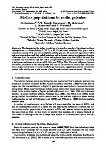
Observations were made with the Wide Field Planetary Camera 2 of the Hubble Space Telescope between May 1994 and December 1995 through the F555W (∼ V ) and F814W (∼ I) filters. Total exposure times were 4000s, 2500s, and 1000s in each filter for Fields 1, 2, and 3, respectively. Observations through each filter were split into three or more separate exposures to allow identification and removal of cosmic ray events. In Figure 1, an image of the LMC shows the approximate positions of the three fields. A previous analysis of Field 1 has been presented by Gallagher et al. (1996) and Holtzman et al. (1997). The positions and exposure times for each field are listed in Table 1. The data were processed using standard reduction techniques described in Holtzman et al. (1995a). This process includes a small correction for analog-to-digital errors, overscan and bias subtraction, dark subtraction, a small shutter shading correction, and flat fielding. In each filter, the images were combined and cosmic ray events were removed based on the expected variance from photon statistics and read noise.

2.1.

Photometry

A combination of profile-fitting and aperture photometry was chosen to give good photometry at both bright and faint signal levels. Since the F555W and F814W images were roughly equally deep, stars were found for each field on the summed frame of these two images. Due to structure in the point spread function (PSF), objects found in the area surrounding the peak of bright stars were rejected. Using this star list, profile-fitting photometry was performed on each frame. The model PSFs were the same as those used by Holtzman et al. (1997). Profile-fitting results were then used to subtract all stars from the images. Final magnitudes were determined by adding each star individually back into the subtracted frame and performing aperture photometry with a 2 pixel radius aperture. Aperture corrections to a 0.5 arcsecond radius aperture were individually determined for the four WFPC2 chips from bright, isolated stars. We estimate the maximum error of this correction to be a few hundredths of a magnitude. Instrumental magnitudes were transformed into V and I magnitudes using the transformations given by Holtzman et al. (1995b). To convert into absolute magnitudes, we adopt a distance modulus of 18.5 derived by

–5– Panagia et al. (1991) from SN1987A . A re-evaluation of the Cepheid distance calibration, using Hipparcos parallaxes, suggests a slight upward revision in the LMC distance modulus to 18.57 ± 0.11 (Madore & Freedman 1997), however, our conclusions are insensitive to errors of this order in the distance modulus. Schwering & Israel (1991) determine a foreground reddening of E(B − V ) = 0.07 towards Field 1 and variations less than 0.02 in E(B − V ) between the three fields. Allowing for a small amount of internal extinction, we adopt E(B − V ) = 0.1 with a corresponding extinction of AV = 0.31. To estimate completeness, a set of artificial stars tests was performed. At a series of different brightnesses, artificial stars were added to each frame in an equally spaced grid and the frames were run through the photometry routine described above. The grid spacing was chosen so that artificial stars did not add significantly to crowding in the field; 121 stars were placed on the PC and 529 stars on each of the WFs. The resulting photometry list was compared to the input list and the completeness level was determined as described by Holtzman et al. (1997). We estimate the 90% completeness level to be at mV ∼ 26 in Fields 1 and 2, and mV ∼ 24.5 in Field 3 due to the lower exposure time. We restrict our analysis to stars brighter than these limits. The fraction of detected artificial stars and their associated errors were tabulated as a function of magnitude and are used in §4.2 to simulate observed stellar populations. These errors include systematic errors due to crowding and random errors from Poisson statistics. Observational errors for our simulations (discussed below) are determined by randomly sampling from these error distributions. The stellar density in these regions of the LMC is low and the fields are not crowded (see Holtzman et al. 1997 for an image of Field 1). For stars brighter than mV ≤ 18.0, our observations are not representative due to saturation and the small WFPC2 field of view. In §4.2, we correct for small number statistics at the brightest magnitudes using ground based data taken with the Mount Stromlo and Siding Spring Observatories 1m telescope (Stappers et al. 1997). Three fields adjacent to and including Field 1 were observed in V and I. The exposure time for each field was 1000s in each filter. The total area on the sky, excluding a region around the cluster NGC 1866 and a second smaller cluster, was 622 arcmin2 . Reduction and photometry were done using standard IRAF tasks. These data are complete to an apparent magnitude of mV ≈ 21. Photometric consistency between the ground-based and WFPC2 data was checked by comparing 37 stars common to both; differences in V and I were 0.0 ± 0.1 magnitudes.

3.

COMPARISON BETWEEN THREE LMC FIELDS

–6– 3.1.

Color-Magnitude Diagrams

Color-magnitude diagrams (CMDs) for the three WFPC2 fields are shown in Figure 2. The faintest main sequence turnoff for the three fields occurs at MV ≈ 3.5, and a clear main sequence extends roughly four magnitudes fainter. The number of stars in each field is roughly comparable. Error bars plotted in Figure 2 are average one σ errors as determined by the aperture photometry routine. Larger errors in Field 3 are a result of the shorter exposure time. Major features in these CMDs, such as the main sequence, the main sequence turnoff, and the red giant branch, occur at the same magnitude and color, suggesting similar stellar populations. We first compare stellar distributions across the lower main sequence as these are sensitive to metallicity variations between the three populations. We then compare the distributions across the upper main sequence as these probe variations between the recent star formation histories of the three fields. As a statistical test of comparison, we use the one dimensional Kolmogorov-Smirnov (KS) test. This test is used to compare the three fields, as well as to compare the observed luminosity functions to simulated stellar populations. The KS test gives the probability (P) that the deviations between two distributions are the same as would be observed if they were drawn from the same population. Two distributions are considered different if the probability that they are drawn from the same parent distribution can be ruled out at a confidence level greater than 95% (P ≤ 5%). If two distributions cannot be proved different, we infer that the populations are similiar, although the KS test does not imply that these distributions are the same. We estimate the sensitivity of this test to minor differences in the star formation history using simple simulations described below. As seen in Figure 2, stars appear to be concentrated towards the blue side of the lower main sequence. The lower main sequence of Field 1 appears the most concentrated towards the blue, Field 3 appears the least concentrated. For Field 3, this is likely the result of a lower exposure time, but for Field 2 may reflect a real difference with the stellar population in Field 1. The histograms of Figure 3 plot the color distributions for Fields 1 and 2 in several magnitude bins across the lower main sequence. The total number of stars in each histogram has been normalized to the number in Field 1. We used the KS test to statistically compare the distribution of stars across the lower main sequence in these fields. In Figure 3, the relatively high values of the KS probability, P= 0.2, 0.3 and 0.9, indicate that we cannot demonstrate that the two samples are drawn from different populations. The signal-to-noise in Field 3 is lower due to a shorter exposure time. In order to compare lower main sequence distributions, we add gaussian noise to the higher signal-to-noise Field 1 using the average errors from Field 3 and perform the KS test. In Figure 4, the distribution of lower main sequence stars in Field 3 is compared to the Field

–7– 1 plus noise distribution. Again, we cannot prove that the distributions are different at a high confidence level. The application of the KS test to the lower main sequence color distributions is weakened by the small number of stars in each comparison, however, it does suggest similar stellar populations in the three field. Although the distribution of stars will also be influenced by age variations and the presence of binaries, the similarity in the mean colors of the lower main sequences suggest that the three fields have similar mean metallicities. To estimate the sensitivity of our tests to differences in metallicity, we use stellar models described below to simulate stellar populations with identical star formation histories but different metallicity distributions. We find that the KS test is sensitive to metallicity differences if, between the two populations, at least 25% of the stars have a factor of four difference in metallicity. This fraction decreases to 20% of stars if the metallicity differs by a factor of ten. These results are robust for several different assumed star formation histories. From the width of the lower main sequence, we can rule out the possibility that the observed stellar populations have a single metallicity. The standard deviations of the observed lower main sequence distributions shown in Figure 3 are σ(V −I),observed = 0.06, 0.07, 0.08 for the three magnitude bins. Field 3 is not included due to the higher noise. We compare this width with that of a simulated single metallicity population, assuming a constant star formation rate from 12 Gyr to the present and a 50% binary fraction. Observational errors are simulated by randomly sampling the error distributions determined from artificial star tests, and include both systematic and random errors. Independent of assumed metallicity, the standard deviation of the lower main sequence was σ(V −I),model = 0.05, 0.05, 0.06 for the same magnitude bins. We find that the difference between the observed and model variances is significant based on a F-test. Populations having a smaller age range or a lower assumed binary fraction will have narrower distributions. Therefore, the observed lower main sequence is wider than is expected for a single metallicity population. Since this is a differential comparison, we expect it to hold regardless of the adopted stellar models. The derivation of the absolute metallicity is discussed in §4.1 and may be model dependent. The distribution of stars across the upper main sequence is shown in Figure 5. The width of the main sequence is broader than would be expected from a single age population. From stellar evolution models, stars brighter than MV ≈ 3 evolve steadily redward during their main sequence lifetimes. Thus, a uniform distribution across the upper main sequence suggests no intense star formation bursts have occurred during the lifetimes of these more massive stars. Gallagher et al. (1996) show that the distribution of upper main sequence stars in Field 1 is roughly consistent with a star formation rate constant for the past 3

–8– Gyr. The KS test gives no evidence that the distributions of stars across the upper main sequence in the three fields are different. This test is not sensitive to variations in the star formation history more recent than 0.1 Gyr, due to small number statistics at the brightest magnitudes. A second distinct main sequence turnoff discussed by Gallagher et al. (1996) and seen near MV ≈ 2.5 in Figure 2a is not observed in the remaining two fields. Gallagher et al. interpret this turnoff and associated excess of stars at MV = 2 in the Hertzsprung gap as signatures of a short star formation burst occurring ∼ 2 Gyr ago. Although many stars populate this region of the CMDs in Field 2 and 3, the lack of a single distinct subgiant branch in these fields argues against a short (t ≤ 0.1 Gyr), global 2 Gyr burst throughout the LMC. The subgiant excess observed in Field 1 may arise from a statistical fluke, the remnants of a localized star formation burst, or a dissolved cluster.

3.2.

Comparison of Luminosity Functions

The observed, uncorrected, differential luminosity functions are shown in Figure 6. We perform the KS test between Fields 1 and 2 over the range −0.5 ≤ MV ≤ 7.5 and between Field 1 and Field 3 over the range −0.5 ≤ MV ≤ 6. The resulting KS probabilities between fields are PLFF ield1−2 = 0.37 and PLFF ield1−3 = 0.26, thus we are not able to show that the three luminosity functions are different.

3.3.

Summary of Comparison

We conclude, from analysis of the luminosity function and distribution of stars across the main sequence, that the three observed regions in the LMC field contain statistically indistinguishable stellar populations. In addition, we have calculated R-ratios as defined by Bertelli et al. (1992) and discussed below (§4.2), which compare the number of stars in different evolutionary phases; these are shown in Table 2. These ratios are also the same between the three fields, within the errors determined by number statistics. We cannot prove that the star formation histories in the three fields are different; however, this does not imply that they are identical. To estimate the sensitivity of our tests to variations in star formation history, we simulate a simple star formation history with a constant star formation rate. We compare this to models in which star formation is turned off completely for short lengths of time at different epochs. We find that our statistical tests are unable to conclusively distinguish between such models for variations in star formation

–9– rate over periods shorter than 1 Gyr anytime in the past 4 Gyr, or over periods shorter than 2 Gyr anytime before 4 Gyr ago. We next compare our observations to stellar models using similar statistical tests in order to place constraints on possible star formation histories. As we have shown that our methods cannot distinguish between the three stellar populations, we combine the observations of the three fields to improve number statistics.

4.

STAR FORMATION HISTORY 4.1.

Stellar Models

To determine the star formation history in the three fields, we compare our observations to simulations made using the stellar evolution models published by the Padua group (Bertelli et al. 1994 and references therein). These isochrones range in metallicity from 0.0004 ≤ Z ≤ 0.05 (-1.7≤ [F e/H] ≤0.4) and are calculated for stellar masses down to < 8, 0.6M⊙ . Depending on the metallicity, this corresponds to an absolute magnitude of MV ∼ roughly the magnitude limit of our observations. The Padua models are calculated with mild convective overshoot and the most recent Livermore group radiative opacities (Iglesias et al. 1992). UBVRI magnitudes for these models have been calculated by Bertelli et al. (1994). There is evidence for nonsolar abundance ratios in the LMC, such that the α-element are enhanced relative to the solar ratio (Luck & Lambert 1992). Although α-enhanced models are not currently available, Salaris et al. (1993) have found that under some conditions, α-enhanced isochrones are well mimicked by scaled solar metallicity isochrones. The effect of α-element enhancement is to shift a solar abundance isochrone towards the red, which would lead to an overestimate of our derived metallicities. Comparing the observed CMDs to single age isochrones, we find the blue edge of the upper main sequence is best matched by an isochrone of metallicity Z=0.008, whereas the red giant branch can be fit by either an old to intermediate age, metal poor isochrone (t ≥ 2 Gyr and Z=0.0004) or a young, higher metallicity isochrone (t ≤ 2 Gyr and Z=0.001). This point is well illustrated in figure 4 of Holtzman et al. (1997). Problems with the stellar atmospheres at lower temperatures and/or the evolutionary models of giant stars may be responsible for the apparent mismatch. Alternatively, it may be related to our use of solar abundance ratio isochrones. Because of these possible problems, we do not use the color of the giant branch to derive stellar population parameters. However, some of the derived parameters, in particular metallicities, are sensitive to the model colors of main sequence stars. We note that our constraints on such parameters are derived assuming that

– 10 – these stellar models are perfect; we allow for random errors in the observations but not for systematic errors in the models.

4.2.

Simulations

The presence of a bright main sequence, seen in Figure 2, suggests recent star formation activity, whereas the faintest main sequence turnoff at MV ≈ 3.5 implies an older star formation epoch. We therefore simulate CMDs for a mixture of simple stellar populations. Throughout the simulations, we assume that 50% of the stars are binaries with uncorrelated masses (Reid 1991). In order to preserve isochrone shape during age interpolation, each isochrone is resampled into 100 equally spaced mass points within each of 9 evolutionary epochs. No interpolation is made in metallicity. The mass and age of each star are chosen according to an input initial mass function and star formation history. The absolute magnitude and color of each star can be determined for any desired age by interpolating point by point over the resampled isochrones. An apparent magnitude is determined based on the extinction and distance modulus. The star is considered detected or rejected according to the completeness histograms calculated during the artificial star tests described above. An observational error is given to each detected star by randomly sampling the error distribution appropriate for the star’s magnitude determined from the artificial star tests (see §2.1). These errors include both random and systematic effects. The number of free parameters in determining a star formation history is large. Our observations do not provide enough constraints to justify an exhaustive search of parameter space. Instead, we choose to discuss six representative formation histories: constant star formation throughout the history of the LMC, the two preferred histories of Bertelli et al. (1992) and Vallenari et al. 1996b, two proposed histories of Holtzman et al. (1997), and a formation history motivated by the observed age distribution of LMC globular clusters. In all cases, we assume the age of the oldest LMC stars to be 12 Gyr based on age estimates of the oldest LMC globular clusters (van den Bergh 1991). The parameters used in each simulation are shown graphically in Figure 7. To compare observed and theoretical stellar populations, we use a combination of two methods. First, we compare observed and model luminosity functions using the 1-D KS test as described in §3.1. The three fields are combined to create the observed luminosity function and are compared with models over a range −0.5 ≤ MV ≤ 6. A star formation history is considered acceptable if the probability, P, that the luminosity function is drawn from the same population is greater than 5%. The sensitivity of this test to variation in the star formation history is the same as that discussed in §3.3.

– 11 – In comparing luminosity functions without regard to color, some star formation history information is lost, especially for stars brighter than the main sequence turnoff. Thus, in addition to luminosity function fitting, we use the R-method described in detail by Bertelli et al. (1992) for MV ≤ 3. Briefly, this method defines three stellar number ratios, each sensitive to different parameters in the star formation history. The first ratio is defined as: R1 =

# of main sequence stars , MV ≤ 3 # of red giant stars

(1)

The separation between main sequence and red giant stars is determined by the lines shown in Figure 2, and is consistent throughout the analysis. The next two ratios compare the number of bright to faint stars on the main sequence and the red giant branch. The magnitude separating the upper and lower regions is defined at MV = 1.5, chosen to be below the red clump. The ratios are defined as: # of upper red giant stars (MV ≤ 1.5) # of lower red giant stars (1.5 ≤ MV ≤ 3)

(2)

# of lower main sequence stars (1.5 ≤ MV ≤ 3) # of upper main sequence stars (MV ≤ 1.5)

(3)

R2 =

R3 =

The R-ratios depend, in different ways, on the slope of the initial mass function and the relative number of young and old stars; see Bertelli et al. (1992) for a more extended discussion of these dependencies. The R-ratios for the three observed fields, as well as the ratios resulting from combining the three fields, are shown in Table 2. The errors in this table are one σ errors as determined from number statistics. The WFPC2 fields do not provide representative numbers of stars at the brightest magnitudes due to saturation and the small field of view. We corrected for this by combining the HST data with ground-based data covering a significantly larger field and including Field 1. A more detailed analysis of these data was presented by Stappers et al. (1997). To combine star counts from ground and space-based data directly, we applied a scale factor determined by the ratio of observed areas. We use ground-based star counts for magnitudes brighter than MV = 1.5 to recalculate the R-ratios of the combined field. As compared to the uncorrected ratios (Table 2, second to last row), the use of ground-based data results in an average 10% corrections to the R-ratios (Table 2, last row). Constraints from the R-ratios, particularly R2 , may be less secure than those based on the main sequence because of the larger uncertainties in modelling later phases of stellar evolution.

– 12 – 4.3.

Star Formation History

We compare the observed luminosity function and R-ratios with those calculated for the six star formation histories shown in Figure 7. The observed and computed R-ratios, as well as the KS probability resulting from a comparison of the observed and model luminosity functions, are given in Table 3. The observed and simulated luminosity functions for each model are shown in Figure 8. The simulated luminosity functions are normalized to match the observations at MV = 4. The simplest star formation history tested assumes a Salpeter IMF and a constant star formation rate since the formation of the LMC 12 Gyr ago (Figure 7a). In examining the parameter R1 , this simple formation scenario does not produce enough bright main sequence stars by more than a factor of two relative to the number of observed evolved stars. This deficiency has motivated most modelers to include an enhancement in the recent star formation rate. Bertelli et al. (1992) observed a field 17′ southwest of Field 1. Using the R-method, they derive a star formation history in which the star formation rate was initially low and then increased by a factor of ten 4 Gyr ago, as shown in Figure 7b. Although this model reproduces the observed R-ratios reasonably well, it does not match the observed luminosity function. As shown in Figure 8b, this formation scenario produces too many bright (MV ≤ 3) stars relative to faint stars. We note that the 1992 Padua stellar models used to derive this history allow for more convective overshoot than the 1994 models used in this paper. The use of more recent models decreases the inferred time when the star formation increase rate began to approximately 2 Gyr ago (Bertelli, private communication). Such a star formation history was used by Vallenari et al. (1996b) to match observations in several of their fields and its luminosity function is shown in Figure 8c. It produces even more bright stars relative to the number of observed faint stars, and is ruled out by our observed luminosity function. In their simulations, Vallenari et al. allow for interpolation in metallicity, whereas our models use discrete metallicity isochrones. We find that the luminosity functions of the three individual metallicities which contribute to the final formation scenario are inconsistent with the observations in the same direction as the composite Vallenari et al. luminosity function. Therefore, this simplification is not the source of discrepancy between the Vallenari et al. scenario and our observations. Holtzman et al. (1997) find that a steeper IMF slope is necessary in order for a 4 Gyr, ten-fold star formation rate increase to match the observed luminosity function. For an IMF slope α = −2.75, this star formation history (Figure 7d) is consistent with the observed

– 13 – luminosity function, but not with the R-ratios observed in our fields. Of published star formation histories for the LMC field, the only one which reproduces both the luminosity function and R-ratios of our observation is that of Holtzman et al. (1997). In this formation scenario, the star formation rate remains constant for a majority of the LMC history and is increased by a factor of three from 2 Gyr ago to the present; the star formation rate is also slightly higher for the oldest stars (Figure 7e). In contrast to the previous three scenarios which produce primarily young stellar populations, this star formation history produces a population with roughly equal number of stars older and younger than 4 Gyr. The simulated CMD for this star formation history is shown in the right panel of Figure 9. A star formation history based on the age distribution of LMC globular clusters cannot fit the observed field population. The age distribution of LMC clusters is bimodal (Figure 7e) with ≥ 90% of clusters formed between 106 years and 3 Gyr ago, and ≤ 10% of clusters having ages between 10 and 12 Gyr (van den Bergh 1991). There are almost no known intermediate age (3-10 Gyr) clusters in the LMC (Girardi et al. 1995; however see Sarajedini et al. 1995), however, an intermediate population is necessary to reproduce our observations. If no clusters have been destroyed, we conclude that the star formation history of LMC globular clusters is not mimicked by the field population.

4.4.

Chemical Evolution

It is possible to predict the chemical history of the LMC from its star formation history using the simple closed box model of chemical evolution. We assume a one-zone evolution model with no infall or outflow, zero initial metal content and instantaneous recycling (Searle & Sargent 1972). This model has successfully predicted the relationship between metallicity and current gas fraction in Magellanic irregular galaxies, although it has less success predicting this relationship in larger spiral systems (Binney & Tremaine 1987). We assume a present day gas to total LMC mass ratio of Mgas /Mtotal = 0.2 (Cohen et al. 1988) and an effective yield of p = 0.005, chosen so that the present day metallicity matches that inferred from the upper main sequence (Z = 0.008). We compare the predicted chemical evolution for two star formation histories in Figure 10. In the upper panel of Figure 10, the Holtzman et al. (1997) star formation history suggests that the metallicity in the LMC has doubled in the past 2 Gyr. The Vallenari et al. (1996) formation history (bottom panel) implies a factor of five metallicity increase in the past 2 Gyr. The chemical evolution predicted by the Holtzman et al. model is consistent

– 14 – with planetary nebula observations by Dopita et al. (1997) which suggest the metallicity of the LMC has almost doubled in the last 2 Gyr. We also note that a significant metal poor population is predicted by the closed box model, regardless of the details of the star formation history. For an effective yield of p = 0.005, the closed box model predicts 22% of stars have metallicities less than Z=0.001. This fraction is inversely proportional to the assumed yield. Simulated lower main sequences suggest a similar fraction of LMC field stars are metal poor. Lower main sequence cross sections are shown for two star formation histories in Figure 11. In the left column, Vallenari et al. ’s model assumes a metallicity range Z=0.008-0.001. These distributions are displaced to the red of the observations by as much as a tenth of a magnitude and are significantly narrower. Although some redward evolution occurs for low mass stars during their main sequence lifetime, changing the star formation history alone is not enough to explain this color shift. The Holtzman et al. model is better able to fit the lower main sequence, as it includes an old, metal poor component as shown in the right column of Figure 11. In this simulated population, 20% of stars have a metallicity Z=0.0004 ([Fe/H]= -1.7). None of the models considered here, however, include chemical evolution in a fully self-consistent manner. Direct measurements of metallicity in the LMC field have been limited to bright stars, but possibly suggest a similar fraction of metal poor stars. Olszewski (1993) spectroscopically determined metallicities for 36 red giant stars in an outer LMC field near NGC 2257 and found that 8 or 9 (∼ 25%) of these stars had metallicities below Z=0.001 ([Fe/H]= -1.3). More metallicity observations are needed to determine the size of a metal poor component in the LMC field (Suntzeff 1997).

5.

SUMMARY

We present deep WFPC2 observations of three fields in the outer disk LMC. We find no conclusive evidence for variation in the stellar populations between the three fields based on the morphologies of the color-magnitude diagrams, the luminosity functions, and the relative numbers of stars in different evolutionary stages. In apparent contrast to our results, Vallenari et al. (1996b) find significant variations in the star formation history correlated with azimuthal angle in the LMC field. A direct comparison with their results, however, is difficult. The R-ratios of our Field 1 agree with those calculated for the nearly overlapping Vallenari et al. NGC 1866 field. Field 3 is located reasonably close to Field 1, therefore the similarity of this field to Field 1 provides

– 15 – no direct contradiction with the Vallenari et al. results. A direct discrepancy comes from Field 2, which is located ∼ 1◦ from the Vallenari et al. field LMC-61. We find significant disagreement in the ratio R3 between these two fields. This discrepancy may be due to the small difference in location or to some systematic error in one or both of the samples. A much larger survey is required to determine whether a correlation exits between the star formation history and position in the LMC field (Zaritsky, Harris & Thompson 1997). Other evidence that the star formation history varies within the LMC comes from Elson et al. (1997), who present evidence that the stellar population in the LMC bar is different from those presented in this paper. They analyze HST observations for a field in the bar of the LMC and identify additional peaks in the color distribution between 20.0 ≤ mV ≤ 22.5 not associated with the red giant branch or the most recent epoch of star formation. They attribute these peaks to a burst of star formation between 1 and 2 Gyr depending on the assumed metallicity. We do not find evidence for this population in our observed color distribution. Elson et al. associate this population with the formation of the LMC bar. We have compared our observations with stellar models to place constraints on possible star formation histories in the three fields. These constraints are an improvement over previous results as they incorporate both HST and ground-based data, allowing measurements of the deep main sequence luminosity function, the distribution of stars in the upper main sequence band, and the relative number of bright stars which probe different evolutionary phases. Of previously considered star formation histories, the only one which is consistent with all of our observations has a star formation rate which is roughly constant for 10 Gyr, then increases by a factor of three for the past 2 Gyr. Contrary to many previous models, this produces a population which is not dominated by young stars. Although the star formation history of the LMC is clearly more complicated, this simple picture should provide a useful guide to understanding the formation of our nearest neighbor. This work was supported in part by NASA under contract NAS7-918 to JPL and a grant to M.G. from the New Mexico Space Grant Consortium.

– 16 – REFERENCES Bertelli, G., Bressan, A., Chiosi, C., Fagotto, F. & Nasi, E. 1994, A&AS, 106,275 Bertelli, G., Mateo, M., Chiosi, C., & Bressan, A. 1992, ApJ, 388, 400 Binney, J. & Tremaine, S. 1987, Galactic Dynamics, (Princeton University Press: Princeton, N.J.) Cohen, R. S. et al. ApJ 331, L95 Dopita, M. et al. 1997, ApJ, 474, 188 Elson, R., Gilmore, G. & Santiago, B. 1997, MNRAS, 289, 157 Gallagher, J. S., et al. 1996, ApJ, 466, 732 Girardi, L. et al. 1995, A&A, 298, 87 Iglesias, C. A., Rogers, F. J., & Wilson, B. G. 1992, ApJ, 397, 717 Holtzman, J. A. et al. 1995a, PASP, 107, 156 Holtzman, J. A. et al. 1995b, PASP, 107, 1065 Holtzman, J. A. et al. 1997, AJ, 113, 656 Luck, R. E. & Lambert, D. L. 1992, ApJS, 79, 303 Madore, B. & Freedman, W. 1997 ApJL, in press Olszewski, E.W. 1993, in ASP Conf. Proc. 48, The Globular Cluster-Galaxy Connection, ed. G. Smith & J. Brodie (San Francisco:ASP), 351 Panagia et al. 1991, ApJ, 380, L23. Perryman et al. 1995, A&A, 304, 69. Reid, N. 1991 AJ, 102, 1428. Sandage, A. 1961, The Hubble Atlas of Galaxies, (Carnegie Institution of Washington: Washington, D.C.) Sarajedini, A., Lee, Y., Lee, D. 1995 ApJ 450, 712 Schwering, P. G., & Israel, F. P. 1991, A&A, 246, 231 Searle, L., & Sargent, W. L. W. 1972, ApJ, 173, 25 Salaris, M., Chieffi, A., & Straniero, O. 1993, ApJ, 414, 580 Stappers, B. J., et al. 1997, PASP, 109, 292 Stryker, L., 1984, ApJS, 55, 127 Suntzeff, N. 1997, Bull. A. A. S., 190, 3501

– 17 – Vallenari, A., Chiosi, C. Bertelli, G., & Ortolani, S. 1996a, A&A, 309, 358 Vallenari, A., Chiosi, C. Bertelli, G., Aparicio, A., & Ortolani, S. 1996b, A&A, 309, 367 van den Bergh, S. 1991, ApJ, 369, 1 Westerlund, B. E., Linde, P. & Lynga, G. 1995, A&A, 298, 39 Zaritsky, D. Harris, J., & Thompson, I. 1997, astro-ph/9709055

This preprint was prepared with the AAS LATEX macros v4.0.

– 18 – Fig. 1.— Image of the LMC showing the approximate positions of the three HST fields. Field 1 is off the image roughly the length of the arrow in the direction indicated. North is up, East is to the left. Taken from Sandage (1961). Fig. 2.— Color magnitude diagrams for Field 1, 2 and 3. One σ error bars are shown as determined by the aperture photometry routine. The vertical solid line is the boundary between main sequence and evolved stars used to determine the R-ratios. Horizontal lines at MV = 3 and 1.5 denote the faint magnitude limit and the separation between bright and faint stars used in the R-method, respectively. Fig. 3.— Histogram of stars across the lower main sequence for three magnitude bins. The solid histogram corresponds to Field 1, the dotted to Field 2. The distributions are statistically indistinguishable as shown by relatively high values of P, the KS probability. The number of stars in Field 2 have been normalized to Field 1. The error bars show one σ errors. Fig. 4.— Comparison of lower main sequence distributions between Field 1 (solid histogram) and Field 3 (dash-dotted histogram). For comparison, gaussian noise has been added to Field 1. Fig. 5.— Distribution of stars across the upper main sequence. In the first column, Field 1 (solid histogram) is compared with Field 2 (dotted), in the second column, Field 1 (solid) is compared to Field 3 (dash-dotted). At these magnitudes, photometry errors in the three fields are much smaller than the bin size. Fig. 6.— The three observed luminosity functions. Field 3 has been normalized arbitrarily. Fig. 7.— Schematic representation of the six star formation histories tested. The initial mass slope, α, is given in the upper right corner, the metallicity is shown above each epoch.

Fig. 8.— Luminosity functions for the six star formation histories compared to the observed luminosity function of the three fields. Model luminosity functions are normalized to match the observations at MV = 4. Fig. 9.— Left panel: Observed CMD for the combined fields. Right panel: Simulated CMD resulting from our preferred star formation history (model (e), Holtzman et al. ). Fig. 10.— Chemical evolution of the LMC predicted by the closed box model for two star formation histories. The model assumes a present day gas mass to total mass of 0.2 and an average effective yield of p = 0.005.

– 19 – Fig. 11.— Comparison of the observed lower main sequence distribution (solid histograms) to two model distributions. A metal poor component is needed to match the observed color distribution.

– 20 – Table 1. Summary of Observations Field α2000 h Field 1 5 14m 44s Field 2 5 58 21 Field 3 5 4 14

δ2000 −65◦ 17′ 43′′ -68 21 18 -66 35 2.4

Exposure time 4000s 2500s 1000s

Table 2. Observed R-Ratios Field Field 1 Field 2 Field 3 Combined Fields Combined + Ground

R1 5.63 ± 0.89 4.30 ± 0.73 4.81 ± 0.72 4.84 ± 0.34 4.24 ± 0.18

R2 1.80 ± 0.70 1.72 ± 0.63 1.89 ± 0.63 1.81 ± 0.24 2.22 ± 0.24

R3 3.49 ± 0.68 3.20 ± 0.64 3.63 ± 0.63 3.46 ± 0.24 3.43 ± 0.12

Table 3. Model star formation results Model Observed Values Constant Star Formation Bertelli et al. (1992) Vallenari et al. (1996b) Holtzman et al. (1997) α = −2.75 Holtzman et al. (1997) α = −2.35 LMC Cluster Age Distribution

R1 R2 R3 4.24 ± 0.18 2.22 ± 0.24 3.46 ± 0.12 1.97 ± 0.05 1.02 ± 0.04 4.02 ± 0.14

PLF 9 × 10−9

4.00 ± 0.08 1.90 ± 0.07 3.84 ± 0.09 2 × 10−11 5.55 ± 0.12 3.39 ± 0.15 2.98 ± 0.06

≤ 10−11

3.06 ± 0.08 1.45 ± 0.07 4.49 ± 0.15

0.14

4.02 ± 0.09 2.08 ± 0.09 3.41 ± 0.08

0.17

9.53 ± 0.17 3.32 ± 0.12 2.21 ± 0.03

≤ 10−11

– 21 –

Fig. 2.-

– 22 –

Fig. 3.-

– 23 –

Fig. 4.-

– 24 –

Fig. 5.-

– 25 –

Fig. 6.-

– 26 –

Fig. 7.-

– 27 –

Fig. 8.-

– 28 –

Fig. 9.-

– 29 –

Fig. 10.-

– 30 –

Fig. 11.-