II!ij(x,ui(x)) -!ij(X',Ui(X)) ,
v
II
87
I ~ - eI
(3.67)
.I
obtain lower bound
-11!ij(x',Ui{X)) - fij(X',Ui(X')) II· , v
~
obtain upper bound We next obtain a lower bound for the first term and an upper bound for the second term of (3.67) as indicated. Obtaining the lower bound for the first term requires certain inversions that must be justified via the implicit function theorem. Technical Detail: The Lower Bound for II lij(X, Ui(X)) - lij (X',Ui(X)) II: We use a general notation for these details for the sake of clarity. Consider the two equations
Zl
Z2
F(XI, y), F(X2, y),
where Xi, Zi E IR n - k , i = 1,2, and y E IRk is regarded as a parameter vector. The function F is sufficiently differentiable (say C r , r ~ 2) on an open set where the implicit function theorem can be applied. Using the implicit function theorem, we invert these two equations to obtain
Xl
X2
H(ZI,y), H(Z2, y).
Taylor expanding and subtracting these equations gives
or
88
3. Persistence of Overflowing Invariant Manifolds-Fenichel's Theorem
Translating these estimates into our notation by letting P X2 = X', Y = Ui(X), C- 1 = DP-l, we obtain
II iij(X,Ui(X)) -
iij(X',Ui(X))
II ~ II C- 1 11- 1 11
X-
= iij, Xl = X,
x'II +0 (II X -
X'
11 2).
(3.68) Obtaining an upper bound for the second term of (3.67) is trivial. Taylor expanding this term gives
:::; 8 II E 1111 X - x'II +0 (II x - x' 112) .
(3.69)
Using (3.67), (3.68), and (3.69), we obtain
II' - " II ~ II C- 1 11- 1 11 x - x'II -811 ~II C- 1
11- 1
(1 -
E
1111 x - x'II +0 (II x - x' 112)
8 II c 1111 E II) II x - x'II +0 (II x - x' 112) . (3.70)
Now
II C- 1 11< Q, and we choose x, x' suficiently close so that
o (II x - x' 112) < 8Q II x - x'II· Combining these two estimates with (3.70) gives
II
,-e II~II C-
1
11- 1 (1- 8Q2) II x-x' 11-8Q II C- 1 1111 C- 1 11- 1 11 x-x'II
or
II' -
e II~II C-
1
11- 1 (1 -
Now we return to the main estimate
28Q2)
II x - x'II.
(3.71)
3.3. Statement and Proof of the Main Theorem
89
We Taylor expand each of the two terms in the second line of (3.72) to obtain
I %(X,Ui(X)) -
gij(X/,Ui(X))
II sll A 1111 x -
II gij(X /, Ui(X)) -
gij(X /, Ui(X' ))
(II x -
xiii +0
I sll B II 8 I x -
x' 112),
xiii +0 (II x - x' 112) . (3.73)
Substituting (3.73) into (3.72) gives
I
(GU)j (~) - (GU)j (e')
Now we use the bound so that
lis (II A II + I B 118) I x -
IAI
-
4'
and TJ sufficiently small such that 2TJQ
~
II
(3.79)
I Ui -
I C- 1 11-111 x -
x'
(3.78)
u~
110. This will
II
(3.80)
for x and x' such that
I
10 (11 x-x'1I2)
Next we estimate and II Ui - u~ 110. To this end we have
Illij (x', u~(x')) -
iij (x', Ui(X))
I
x - x'
I
3.3. Statement and Proof of the Main Theorem
91
< liE 1111 U~(X') - u~(x)) I +0 (II U~(X') - U~(X) 112)
< Q (15 I X -
xiii + I U~ -
Ui 110) + 0
(II X -
X' 112) + 0
(II U~ -
Ui 115) . (3.81)
Combining (3.80) and (3.81), and using (3.77), gives ~
I C- 1 11-111 X - xiii :::; Qt5ll X - xiii +Q I U~ - Ui I +0 (II X - X' 112) + 0 (II U~(X) -
Ui(X) 112) ,
from which, for 15 sufficiently small, it follows that
I X-
x' 11< constant
I Ui -
U~ 110 .
Combining this estimate with (3.78) and (3.79) gives
I
(GU)j
For 15 and
(~) -
(GuI)j (()
II:::;
[(21] + ~t5) constant + 196]
1] sufficiently small, it follows that (21] + ~t5)
I Ui - u~ 110 . (3.82)
constant + 196 < 1.
Hence, the proposition is proved.
D
Corollary 3.3.4 There is a unique u E So such that graph u for all t > o.
0 o
Ui(~) - Vi(~) (~ - e) I ~' - ~ II
I
0
=
for every i, which implies that Vi s the derivative of Ui. First, we address a technical issue. Let ~ E V 3 be given and suppose that for some i, j that ~ = fij(X,Ui(X)) with x E V 3. If d is chosen small enough and E V 3 with II ~ I < d, there is an x' E V3 such that = fij(x', Ui(X')). Moreover, by compactness, d may be chosen to be independent of~, i, and j. In other words, fij(x, Ui(X)) is locally onto. This can be shown using an implicit function theorem type argument along with the fact that I (Ddij)-l I is bounded. It will be sufficient to show that
e
e
e
e-
e
for all i, j, ~, satisfying the above requirements with I ~ II:::; a < d. Then the result follows immediately by appealing to Lemma 3.3.8. We begin with some preliminary estimates:
( - ~ =
fij(x', Ui(X')) - fij(X, Ui(X)) C (x' - x) + E (Ui(X') - Ui(X)) +0 (II x' - x 112) ,
(3.110)
9ij(X', Ui(X')) - 9ij(X, Ui(X)) A (x' - x) + B (Ui(X') - Ui(X)) +0 (II x - x' 112) .
(3.111)
From a previous estimate (Eq. (3.71)) we have
I x' -x II:::;
t~;;J~ I (-~ II·
(3.112)
Also, rewriting (3.110) in the following form will be useful: (-~ =
(C+EVi(X))(X-x') +E (Ui(X') - Ui(X) - Vi(X) (x - x'))
+ 0 (II x -
x'
112) .(3.113)
100
3. Persistence of Overflowing Invariant Manifolds-Fenichel's Theorem
We now begin the main estimates.
II A (x -
(II x -
x') + B (Ui(X') - Ui(X)) + 0
- [A + BVi(X)] [C + EVi(X)rl (~- ()
II A (x -
II
from (3.111) and (3.92)
(II x -
x') + B (Ui(X') - Ui(X)) + 0
x' 112)
x' 112)
+E (Ui(X') - Ui(X) - Vi(X) (x - X'))]
II
x [E (Ui(X') - Ui(X) - Vi(X) (x - x'))]
+ 0 (II x -
from (3.113)
x'
112) I
II [B - [A + BVi(X)] [C + EVi(X)rl E]
< (II B II +0(8)h(11 x' -x II) II x' -x II +0(11 x-x' 112) < [(II B I ~~ ;i6~1
C- I
II] 'Y (II x' -
x
II) II e - ~ II +0 (II
x - x'
112) ,
(3.114) where the next to last inequality is obtained by using (3.108) and Proposition 3.3.5, and the last inequality is obtained by using (3.112). Now the goal is to show that (3.114) can be put in the form of (3.109). Recall that
II B 1111 C- I 11< ~; then if we define
_ (II
0:
=
B
II +0 (8)) II 1 _ 28Q2
C- I
I
'
(3.115)
3.3. Statement and Proof of the Main Theorem
it follows that
Q
< 1 for
1],
101
8 sufficiently small. Next we define {3
=
Q
(3.116)
1- 28Q2'
Then from (3.112) we have
I x - xiII::; ,B I e' - e11< ,Ba. Since
(3.117)
'YO is nondecreasing, it follows that 'Y (II x - xiII) ::; 'Y (,Ba) .
(3.118)
From (3.117) it follows that
o (II x' -
x 112) < r(a)
I e' - eI
(3.119)
for some function r(a) where
r(a)
--+
0
as a
--+
O.
Combining (3.114), (3.115), (3.118), and (3.119), we have shown
with the required hypotheses of Lemma 3.3.8. This proves the proposition.
o
cr.
Now we will proceed by induction to show that Mpert is We will next show that Mpert is C 2 . At this step most of the difficulties associated with higher order derivatives will be clear. We will then suppose that Mpert is C P, for 1 < p < r, and show that this implies that Mpert is CP+ 1 . The proof that Mpert is C 2 proceeds by the same steps that we used in showing that Mpert is C 1 • We first derive a functional equation that the second derivative must satisfy and, using an iteration argument, show that this equation has a solution. Finally, we argue that this solution is, indeed, the second derivative. We formally differentiate (3.96) and obtain the following equation which the second derivative must satisfy:
DVj(e) = ~:=1 {D¢i . [A + BVi(X)] [C + EVi(X)r1
+¢i . D {[A + BVi(X)] [C + EVi(X)r1} } [C + EVi(X)r1
= ~:=1 {D¢i . [A + BVi(X)] [C + EVi(X)r1
102
3. Persistence of Overflowing Invariant Manifolds-Fenichel's Theorem
0
as
i
t
00,
Vwo E N;}.
(4.4)
< 1, we then define
(TS(p)
=
inf {b
: (II Wo lib / I Vo II) / (II W-t lib / II V-t II) -> 0 as t i 00, Vvo E TpM2' Wo EN;}.
(4.5)
Following the same calculations as in Lemma 3.1.1, we can show that these expressions are equal to the following:
I ITuDcP_t(p)INu lit,
(4.6)
I ITsDcPdcP_t(p)) INs lit, -1" log II DcP-tIM2(p) II t2.~ -log I ITs DcPt (cP-t(p)) INs
(4.7)
lim
t--+oo
lim
t--+oo
P
P
P
II·
(4.8)
Lemma 3.1.2 (constant on orbits) and Proposition 3.1.3 (independent of metric) also apply to these generalized Lyapunov-type numbers. The proofs involve identical calculations. We say that the splitting is hyperbolic if
VpEM.
(4.9)
4.1. Generalized Lyapunov-Type Numbers
113
The geometrical interpretation of these generalized Lyapunov-type numbers should be clear from the earlier discussion. Moreover, we have the following uniformity lemma due to Fenichel [1971].
Lemma 4.1.1 (Uniformity Lemma for Unstable Manifolds) 1. Suppose
Then there are constants
a < a and C such that
2. Suppose
Then there are constants
a< a and C such that
3. Under the hypotheses of (1), suppose also that a
Then there are constants
b< band C
and
uniformly Vp
E
MI.
1 and
such that
I IIu D¢-t(P)INu 11-40 p
~
as t
i
00,
114
5.
4. The Unstable Manifold of an Overflowing Invariant Manifold
vsO, >,uO,
and
aSO
attain their suprema on M.
Proof: The proof proceeds exactly as in the proof of the uniformity lemma D given earlier.
4.2
Local Coordinates Near M
Next we need to construct local coordinates near M 2 , describe the flow in these coordinates, and set up the graph transform. Much of the construction will be similar to that given earlier, so we will not give all the details. We begin by constructing a neighborhood of M. The dimension of N; will be s and the dimension of N; will be u. Hence, the dimension of M will be n - (s + u). Following Proposition 3.2.3, we perturb the bundles N S and NU to C r bundles N's and N'u, respectively. Perturbation of the Subbundles N S and N U : Proposition 3.2.3 showed how the C r - l normal bundle N could be perturbed to a C r tmnsversal bundle N ' . Exactly the same argument applies to N == N B EB N U. Following the same notation as in Proposition 3.2.3, we define maps u
M2
-+
G(u, n),
B
M2
-+
G(s, n).
Following exactly the same arguments, one can construct C r maps ~u and ~B that are arbitrarily CO close to u and B' respectively, on Ml . One can then conclude that there are C r subbundles N 'U and N'B that are CO E-close to N U and N B, respectively, with N ' == N'U EB N'B. Moreover, N'U and N'B have C r orthonormal bases.
We then define =
{ (p, VB) EN'S : I
VB
I ~ E} ,
{(p,V S ) E N'u : I VU II~
E},
and the map h
N,B€
ffi CD
N'u€
--t
IRn ,
(p,VS,V U) t-+ p+v B+v u .
(4.10)
From Proposition 3.2.4 it follows that there is an EO > 0 such that for all E ~ EO the map h is a C r map, mapping N': EB N'~lu~ u5 onto a ,=1 neighborhood of Ui'=l Ot.
o
there exists that if II (rn- 1 (y) 11< f and II (r;,,)-1 (z) 11< f, then we have
f
> Osuch
II g?j(x,y,z) 11< 'fJ, II h?j(x,y,z) 11< 'fJ,
(4.19)
II D 1g?j(x,y,z) 11< 'fJ,
Estimates Derived from the Overflowing Invariance of T M2 EEl N S and TM2 EEl N U Under the Linearized Dynamics First note that in the title of this subsection we have used NS and NU rather than N'S and N 'u . This technical distinction is important as T M2 EEl N S and TM2 EElNu are overflowing invariant under the linearized dynamics; T M2 EEl N's and T M2 EEl N'u need not be. The derivative of the time-T map in the local coordinates (which were defined using N's and N'U) is
Dd&
D2!&
D3f&
( D 1g?j
D 2 g?j
D3g?j
D 1 h?j
D 2 h?j
D3 h?j
1 ,
(4.20)
where we have (for the moment) deliberately omitted displaying the points at which the entries of this matrix are evaluated. In local coordinates the fibers of N's are denoted by (x, y, 0) and the fibers of N'u are denoted by (x,O,z).
118
4. The Unstable Manifold of an Overflowing Invariant Manifold
Now suppose that we instead have used NS and N U to construct local coordiantes for the representation of the time-T map. Then invariance of NS under the linearized dynamics implies that
D 1 h?j(x, y, 0)
= 0,
D2 h?j (x, y, 0)
= 0,
(4.21) and invariance of NU under the linearized dynamics implies that (4.22)
D3g?j(x, 0, z)
= 0.
Now the bundle N's (resp. N'U) can be chosen to be arbitrarily close to NS (resp. NU); hence, for a given TJ > 0, and € sufficiently small, we have
II
D 1 h?j(x,y,z)
11< TJ,
II
D2 h?j(x, y, z)
11< TJ,
(4.23)
II D 1 g?j(x, y, z) 11< TJ, II D3g?j(x, y, z) 11< TJ· A Dilational Estimate
The idea for the following estimate comes from Fenichel [1974], p. 1133. We want to argue that II D3fi~ II can be made small by an appropriate rescaling of the z coordinate. Consider the following dilation of the coordinates:
(x, y, z)
1--+
(x, y, "'z)
=
(x, y, z),
(4.24)
where", is a positive real number. First we want to consider how this dilation will affect the estimates (4.16), (4.19), and (4.23) given above. It is easy to see that it has no effect on the estimates (4.19) derived from overflowing invariance of M under the nonlinear dynamics. The only estimate in (4.23) affected by the dilation of coordinates is II D3g?j(x, y, z) 11< TJ, which becomes II D3g?j(x, y, z) 11< "'TJ in the dilated coordinates. However, the estimates derived from the growth rates, (4.16), require more careful consideration. For these three quantities, one need only worry about terms involving the partial derivative with respect to z ( D 3 ) in particular, the quantity II (D 3h?j(X, 0,0))-1 11< ~. In the dilated coordinates this estimate becomes for", < 1.
II (D3h?j(X, 0, 0)) -1 11< ~,
which is smaller than ~
4.4. The Space of Sections of N'.lu~'1=1 u3 over N':lu~1.=1 u3 t
119
t
Now we turn to the quantity of interest. In the dilated coordinates it becomes K, II D3 f&(x,O,O) II, which clearly can be made arbitrarily small, say less than '1], by taking K, sufficiently small. Henceforth, we will assume that this holds. Moreover, by continuity, we may also further assume that for x and y sufficiently small we have
(4.25) We henceforth assume that we are working in these dilated coordinates and drop the "bar" from our notation on z. In the following arguments we will have reason to refer to the estimates (4.16), (4.19), (4.23), and (4.25) repeatedly. In such instances we will collectively refer to these estimates as the GR-I estimates (Jor "growth rate" and "invariance").
General Bounds We assume that the norms of the first and second partial derivatives, and the inverses (when appropriately defined), of f&, g?j' and h?j are bounded by some constant, say Q. This follows from the fact that these functions are CT and we are restricting ourselves to a compact subset of rn.n .
4.4
The Space of Sections of N'El ui=l Ul over
N'~lui=lUl The unstable manifold of M will be constructed as the graph of a section u of N'.lu~'1=1 u3 over N'~lu~1.=1 u3. However, first we should describe how we view N'. as a vector bundle over N'~. A point in N'. == N'~ EEl N': is denoted by (p,V U ,v8 ), where p E M 2. Thus, viewing N'~ as the base space of the vector bundle N'" a point in N'. is denoted by (p, v U , V S ), where (p, V U ) is regarded as the basepoint. A section of N'. over N'~ is a map t
1.
u : N': (p,V U)
--+
N'"
1--+
(p,VU,V S ),
and let S denote the space of sections of N' .Iu~1.=1 u3 over N'~ lu~1.=1 u3. Local coordinate representations of a section u are given by t
t
120
4. The Unstable Manifold of an Overflowing Invariant Manifold
where and VE == {z E IRu I II z II ~ €}. Since the notation V E arises here for the first time, it is perhaps worthwhile to discuss its origins. According to the above formulas, the domain of the local coordinate representation of U is V3 X VE. This follows from the fact that we are using orthornormal bases to locally describe points in N': and N'~, from which it follows that II rU(p,v U) 11=11 v U 11=11 z II. Using this, we have
Ui
(U!) x rt (N~IUf)
_ vi x V
E,
which is the domain for the local coordinate representation of u. Thus, in coordinates, the section U is represented by the s maps Ui , i = 1, ... , s each defined on V3 x VE. We define
L.
Ipu=m~ t
sup (z,z),(z',z')EV3 XV< (x,z);i(x',z')
II Ui(X, z) - Ui(X', z') II II x - x ' II + II z - z'I' I
(4.26)
if this exists, and denote So = {u E S ILip U ~ 6'} .
(4.27)
Note that we have
II Ui(X, z) -
Ui(X', z') II~ 6' (II x - x'
I + II z -
z'
II)·
(4.28)
It is straightforward to show that So is a complete metric space with the metric derived from the Co norm.
4.5
The Unstable Manifold Theorem
Before stating the unstable manifold theorem we need to address a technical point. Technical Point: If one thinks of the situation of the stable and unstable manifolds of a hyperbolic fixed point of a vector field, the unstable manifold of the fixed point is tangent to the unstable subspace of the linearized vector field, at the fixed point. Similarly, in this general setting, the unstable manifold of M will be tangent to some "linear object" at M-but what is this "linear object"? The obvious candidate is N'~ since trajectories with initial conditions in this bundle have the appropriate asymptotic behavior as t -> -00 and we will construct the unstable manifold as a graph over N/~.
4.5. The Unstable Manifold Theorem
121
However, there is a problem with this choice as the bundle N'~ is not naturally contained in lRn. This issue can be easily handled by embedding the bundle in lRn in a natural way. We define the map
hu : N':
-+
lRn,
(P,V U )
~
p+vu .
Then hu (N'~) C lRn and we can consider the issue of the tangency of the unstable manifold of M and hu (N'~).
We now state the unstable manifold theorem. Theorem 4.5.1 (Fenichel, 1971) Suppose ± = f(x) is a C r vector field on IRn , r ~ 1. Let £II == M U 8M be a compact connected manifold
cr,
with boundary overflowing invariant under the vector field f (x). Suppose vS(P) < 1, ,\u(p) < 1, and (1s(p) < .!r for _all p E M. Then _ there exists a C r overflowing invariant manifold WU(M) containing M and tangent to hu (N'~) along £II with trajectories in WU(M) approaching £II as t -+ -00. Moreover, the unstable manifold is persistent under perturbation in the sense that for any C r vector field fpert(x) C 1 O-close to f(x), with 0 sufficiently small, there is a manifold WU (MPert) overflowing invariant under fPert(x) and C r diffeomorphic to WU (£II). The proof of this theorem will proceed in stages much like the proof of the persistence theorem for overflowing invariant manifolds. We begin by constructing a graph transform and showing that it is well defined. We next show that this graph transform has a fixed point that corresponds to a Lipschitz unstable manifold of £II for the time-T map generated by the flow. We then show that this manifold is invariant for all time. Next, we will turn to the question of differentiability and show that the Lipschitz manifold is actually cr. Finally, we will show that the unstable manifold of £II is persistent under perturbations. The Graph Transform
In local coordinates, the image of a point on graph u is given by
Accordingly, the graph transform is defined by (4.30)
122
4. The Unstable Manifold of an Overflowing Invariant Manifold
where ~c
f~(x, Ui(X, Z), Z),
~u
h?j(x, Ui(X, Z), z).
(Note: The subscript c denotes "center directions." A subscript T for "tangent directions" might have been better, however this could be confused with the T in the time-T map.) Before proceeding we must argue that this map is well defined. The argument is essentially the same as that given using Theorem 3.2.10 and Proposition 3.2.11. We summarize the necessary result in the following lemma.
Lemma 4.5.2 Let
denote the fiber projection map and consider the map
-t
Then for 8 and
E
N ,UE'
sufficiently small, and U
1. X is well defined for all (p, VU ) E 2. U:=l U? x DE eX (Uf=l C Uf=lUi5 X
E
Sli,
0"l X
DE,
ut X DE) ex (U:=l ut x DE)
DE.
3. Each point in Ui=l U? x DE is the X image of only one point in U:=l x DE.
ut
Proof: The proof is identical to the proof of Proposition 3.2.11.
D
A Notational Point: The notation u1 x D€ is not the most mathematically precise since N/~ is not really covered by the sets u1 x De this is just the notation for open sets j which cover N/~ and (since is locally trivial) are diffeomorphic to Dj x D€.
v:
Invariance of the graph implies that the graph transform has a fixed point which is expressed as (4.31)
4.5. The Unstable Manifold Theorem
123
We next want to show that the graph transform has a fixed point. However, we will not do this by proceeding directly with an analysis of the equations in this setup. Rather, we will show that the present setup can be recast into exactly the form of the equations studied when we were proving the existence of an overflowing invariant manifold for the perturbed vector field in Section 3.3. We begin by defining
x-
= ( X,Z,)
-0 (0 ( X,y,Z ) , gij X,Y ) -= gij
(4.32)
with
I x 11= max (II x II, I Z II), (4.33) I ~ 11= max (II ~c II, I ~u II), -00II, 0 II Iij 11= max ( II Iij I hij) I . In these new combined coordinates, x, a section U is locally represented as
Ui(X)
= Ui(X, z).
(4.34)
We introduce the following shorthand notation:
C = Ddg (x, Ui(X))
=
D(1,3) (Jg (x, Ui(X, z), z), h?j (x, Ui(X, z), z)) ,
E = D2~~ (x, Ui(X))
=
(Ddg (x, Ui(X, z), z), D2h?j (x, Ui(X, z), z)) , (4.35)
Estimates for these quantities are given in the following lemma (which is analogous to Lemma 3.2.9). Lemma 4.5.3 For "l, E sufficiently small, and an appropriate constant Q 0, we have the following estimates: 1.
II A II, I B II, II C II, I E I < Q,
>
124
4. The Unstable Manifold of an Overflowing Invariant Manifold
2.
II 0-1 11< Q,
3.
II A 11< 1], II B 11< ~,
4. II B 1111 0-1 11< ~. Proof: Statement 1 follows immediately from the fact that A, B, E are C r - 1 functions defined on a compact domain.
a, and
As for statement 2, we first note that II 0-1 II exists. This follows from the overflowing invariance of T M2 EI1 NU and the overflowing invariance (under negative time) of TM2 EI1 NS under the linearized dynamics as well as from the fact that N's and N'U can be selected arbitrarily Cl close to NS and NU, respectively. But then 0-1 is necessarily a cr-l function and statement 2 follows. Next we turn to the proof of statement 3. First, we can write
(4.36) where we have used (4.23). Second, we have (4.37) which follows from (4.16). This proves statement 3. Finally, we turn to the proof of statement 4. We need to show that
liB 1111 0-1 11=11 D 2 9?i 1111 (DdI~)-1 11=11 D 2 g?i 1111 F- 1 11< ~ (4.38) holds with (4.39) We define (4.40)
c == Dlh?i'
d == D3h?i'
where we have suppressed the arguments and indices for notational simplicity. Note that the GR-I estimates immediately give us
II a 11< Q,
II c 11< 1],
II a-I 11< Q,
II b 11< 1],
II d 11< Q,
II
d- 1
11
-T(p) IN; 11< min { c
a;, ;~} < min {~, sk} ,
I DQ>TIM2 (Q>-T(P)) 1111 IT,uDQ>_T(p)IN; I
0 and .Au > 0 such that max dt < G'e- Aut ,
t E [O,Tj.
O::;t::;T
(5.52)
We want to argue that \It> O.
(5.53)
We will do this by showing that max
(k-l)T::;t::;kT
dt
Goe- Aut for all integers k ~ 1,
:::;
from which (5.53) follows. The argument proceeds as follows. Choose .Au = - log a. Then the constant G' from (5.52) must satisfy
from which it follows that ,11 G > T max dt = T MI· a
(5.54)
a
O::;t::;T
Now from (5.51) and the definition of G for any integer k d
0,
5.6 The Theorem on Foliations of Unstable Manifolds
151
and we take Co = ec'. Thus, we have shown that \I z( -t) - z' (-t)
II:::; Ce- Aut ,
t -+
(5.57)
00,
where, for simplicity of notation, we have omitted denoting the local coordinate changes that may occur as t -+ 00. Furthermore, we can write
II y(-t) -
y'(-t)
II h(z(-t)jp(-t)) -
II
I~(z'(-t)jp'(-t))
I
I{ (z' (-t)j p' (-t))
I
< 811 z( -t) - z'( -t) II,
II x( -t) -
x' (-t)
II
I 11 (z( -t)j p( -t)) -
=
< 811 z(-t) - z'(-t) II,
(5.58)
where, again, for simplicity of notation, we have omitted denoting the local coordinate changes that may occur as t -+ 00. Thus, using (5.57) and (5.58) gives
I ¢-t(q) -
¢-t(q')
11< (; (II x( -t) -
+ II z( -t) -
z' (-t)
x'( -t) \I
+ \I y( -t) -
II) < (;Co(l + 28)e- Aut .
y'( -t) \I
(5.59) By setting Cu = (;Co(l + 28) and q' = p we complete the proof of part 5. PROOF OF PART
6
It is enough to show that as t-+oo and
I ¢-t(q') I ¢-t(p') -
¢-t(p') I -+ 0 as t -+ ¢-t(P) I
00.
This can be seen by noting that
1Iq,-t (q')-q,-t (p')H-t (p')-q,-t (p) II
oo
II (Xk - x~, Yk, Zk) I = 0 I Xk - Xk I
or, equivalently, lim t-->oo
II ¢-t(q) I ¢-t(Pl) -
¢-t(P) I ¢-t(P) I
- 0 - .
The calculation for
proceeds in exactly the same manner. PROOF OF PART
7
The proof is by contradiction. We assume that r(Pl) n r(P2) 3 q but r(Pl) #- r~)· Then there exists q2 E r(P2) but q2 fj. r(Pl), and ql E r(Pl) but ql fj. r~). By part 5 we can write
I ¢-t(q) - ¢-t(P2) I II ¢-t(ql) - ¢-t~) I > lim III ¢-t(q) - ¢-t(ql) II - I ¢-t(ql) - t-->oo I ¢-t(ql) - ¢-t~) II
0= lim hoo
- r
- t2.~
III ¢-t(q) II ¢-t(ql) -
¢-t(ql) I ¢-t(P2) II
-
11
¢-t~)
III
.
This immediately gives (5.67)
I ¢-t(q) - ¢-t(Pt} I I ¢-t(q2) - ¢-t(Pl) II > lim III ¢-t(q) - ¢-t(ql) II - II ¢-t(ql) - t-->oo II ¢-t(q2) - ¢-t(Pl) I
0= lim t-->oo
=
=
lim III ¢-t(q) - ¢-t(ql) I t-->oo I ¢-t(q2) - ¢-t(Pl) II
lim t-->oo
I ¢-t(q) - ¢-t(ql) II I ¢-t(q2) - ¢-t(Pl) II '
_ I ¢-t(ql) I ¢-t(q2) -
¢-t(Pl) ¢-t(Pl) ¢-t(pl)
III III I
5.6 The Theorem on Foliations of Unstable Manifolds
155
which yields lim t-+oo
II cP-t(q) - cP-t(ql) II II cP-t(q2) - cP-t(Pd II
=
o.
(5.68)
=
o.
(5.69)
Combining (5.67) and (5.68) gives lim t-+oo
II cP-t(qd - cP-t(P2) II II cP-t(q2) - cP-t(Pl) II
Since neither Pl or P2 are distinguished, we can interchange the indices in (5.69) to obtain (5.70) Now note that the expressions on the left-hand sides of (5.69) and (5.70) are reciprocals of each other. Hence, we have established a contradiction. PROOF THAT THE FIBERS ARE
Cr
WITH RESPECT TO THE BASEPOINTS
We follow Fenichel [1977]. However, we are able to improve his result slightly in the context of normally hyperbolic invariant manifolds by gaining an extra derivative. If we show that the set E = {(Pl,P2) Ipl EM, P2 E r(pd}
is a C r submanifold of M x JRn , then it follows that the fibers are C r with respect to the basepoint. Let U c JRn be a neighborhood of M in which the family :;:u has been constructed. Note that E is the image of hU(N'U) n U under the map W : hU(N'U) n U
----+
M x lRn ,
(5.71)
(x,z)
f-+
(x,h(z;x),z,h(z;x)),
(5.72)
where we identified the coordinate x of the point P with P itself (see the definitions of h and h). At this point we do not know about the smoothness properties of h(z; x) and h(z; x) with respect to x. However, by construction, we have
Dxh(O;x) Dxh(O;x)
=
Idn-(s+u) ,
=
0,
(5.73)
where Idn-(s+u) denotes the n - (8 + u) x n - (8 + u) identity matrix, a notation that will be used subsequently. Furthermore, since we know that (p) is tangent to N';, we also have
r
Dzh(O;x) Dzh(O; x)
0,
O.
(5.74)
156
5. Foliations of Unstable Manifolds
Based on (5.73)-(5.74), DWI(x,o) exists and equals
I~.) .
Idn-(S+U)
DWI
(x,O)
=
( Idn-(s+u)
0
o
(5.75)
Consequently, E is C l along its subset M* = {(p,p)
Ip EM} c
M x ffin ,
(5.76)
which is just the diagonal embedding of Minto M x ffin. At any point c E the tangent space Tp. E is given by
p* = (p, p) E M*
(5.77) where x is the "tangential" coordinate of p on M. We easily see that M* is an overflowing invariant manifold under the flow
¢; : M x U ¢; (PI, P2)
-t
M x ffi n ,
(¢t(PI), ¢t(P2)) .
We will show that E is a C r submanifold of M x ffin by arguing that E is the unstable manifold of the C r manifold M* under the flow ¢;. To this end, we need to verify the hypotheses of the unstable manifold theorem for M*, which requires the existence of stable and unstable sub bundles NS* and N U *, respectively. The diagonal embedding M* of Minto M x IRn (given in (5.76)) does not tell us how to embed the bundles NS and NU into T(M x ffi n ), hence we must do a separate construction here. It is enough to construct an embedding or Tffi n 1M into T(M x ffin) 1M" because that restricts uniquely to embeddings of its subbundles. At any point P E M, Tffinl p is spanned by the tangent vectors of curves 'Yp : ffi - t ffin , s f-t 'Yp(s), 'Yp(O) = p. Therefore, it is enough to embed curves of this form into M xU. But this can be done easily by defining "I;' = e("{p) with 'Y;'(S) = (p,'Yp(s)),
(5.78)
p* = (p,p),
"I;'
"I;'
where e denotes the embedding map. Now (s) has the property (0) = p*. Using the tangent map of this embedding, we can then embed subbundIes of Tffinl M to obtain subbundles of T (M x ffin) 1M'. In particular, we obtain the splitting
5.7 Persistence of the Fibers Under Perturbations
157
which satisfies the hypotheses of the unstable manifold theorem. Indeed, one can easily check that the type numbers >.u*, v S *, and a s * are the same when computed for this splitting as for the splitting T M EB N U EB N S • We conclude that M* has a CT unstable manifold, WU(M*), which is tangent to h~ (Nu*) along M*, with h~ defined analogously to hu in Chapter 4. The unstable manifold theorem guarantees that WU(M*) has a unique Taylor expansion up to order r. E is clearly overflowing invariant by construction, so if we show that it is tangent to h~ (Nu*) along M*, then it follows that E and WU(M*) must have the same Taylor expansion up to order r; in particular, E is CT. For this it is sufficient to show that Tp. E and Tp. M* EB N;.* coincide for any p* E M*. A coordinate representation of the diagonal embedding of M is given by
M
M
x
-t
M x ffin ,
1--+
(x,x,Ou,Os),
therefore
Tp.M· ~ Range (DM)lp ~ Range
Id,.-r
Idn-(S+U) )
(
kl
.
(5.79)
Selecting u curves, I'p,l(S), ... , I'p,u(s), in Tpffin which are tangent to the elements of the standard orthonormal basis of N'u, respectively, (5.78) gives
N;: ~
Span(:,
~;.,i(O))I~~, ~
Range
(I~' ).
(5.80)
Comparing (5.77), (5.79), and (5.80), we obtain that Tp.E = Tp.M*EBN;.*, which concludes the proof. PROOF OF PART
8
Part 8 is an immediate consequence of the preceeding results.
5.7 Persistence of the Fibers Under Perturbations Exactly the same arguments can be applied as for WU(M) to show that the fibers persist and remain CT under CT perturbations.
6 Miscellaneous Properties and Results In this chapter we collect together a number of useful results, as well as describe several ways the theory can be modified that are important for applications.
6.1
Inflowing Invariant Manifolds
Recall the definition of overflowing invariant manifolds given in Definition 3.0.1. From this definition it should be clear that under time reversal, i.e., t --* -t, an overflowing invariant manifold becomes an inflowing invariant manifold, and vice versa. Thus, if our vector field has an inflowing invariant manifold, then all of the previously developed theory can be applied to the time-reversed flow and its resulting overflowing invariant manifold. In this case, one only needs to take care in the characterization of stability of the inflowing invariant manifold. In particular, in applying the persistence theorem for overflowing invariant manifolds to inflowing invariant manifolds the conditions on the generalized Lyapunov-type numbers characterize an unstable inflowing invariant manifold, and the unstable manifold theorem for overflowing invariant manifolds becomes a stable manifold theorem for inflowing invariant manifolds.
6.2
Compact, Boundaryless Invariant Manifolds
Compact, boundaryless invariant manifolds are both overflowing and inflowing invariant, or according to the terminology of Definition 3.0.1, they are invariant. The persistence theorem, the unstable manifold theorem, the stable manifold theorem discussed above, and the stable and unstable foliation theorems can all be applied to compact, boundaryless invariant manifolds without modification.
160
6. Miscellaneous Properties and Results
6.3
Boundary Modifications
In certain cases, vector fields may possess invariant manifolds with boundary; however, the invariant manifolds are neither overflowing nor inflowing invariant. Rather, the vector field is either tangent to the the boundary or identically zero on the boundary. We give several examples to show that this is not such an uncommon occurrence, and then address the issue of how one deals with this situation in the context of the theory developed in the preceeding chapters. A VECTOR FIELD NEAR A N ONHYPERBOLIC FIXED POINT
Consider the following vector field x = -y + Ej(X, y, z),
iJ = x + Eg(X, y, z),
(6.1)
z = -z + Eh(x, y, z), At
E
= 0 the set
M == {(x,y,z)
E
JR3 1x2 +y2 ~ R, z =
o}
is a two-dimensional normally hyperbolic, attracting, invariant manifold with boundary. The vector field is tangent to the boundary since the boundary is an orbit. A VECTOR FIELD WITH SLOWLY VARYING PARAMETERS
Consider the following Duffing-van der Pol oscillator:
x=y,
(6.2)
0: = 0,
~=o,
l' =
0,
(x, y, a, (3, 'Y)
E
JR2 x K,
where a, (3, 'Y are parameters contained in some compact, connected set K C JR3. Now suppose we consider a situation where the parameters have
6.3. Boundary Modifications
161
their own dynamics, i.e.,
x=y, a=
ff(x, y, ex, {3, "(),
(6.3)
~ = fg(X, y, ex, {3, "(), "y
At by
f
= fh(x, y, ex, {3, "(),
(x, y, ex, {3, "() E
rn? x K.
= 0, (6.3) has an invariant manifold with boundary, denoted
For ex
!VI, given
!VI = {(x, y, ex, {3, "() Ix = y = O}. > 0 this invariant manifold is normally hyperbolic (it is actually
saddle type in stability). The boundary of !VI is given by the boundary of K and it is clear that at f = 0 the vector field is zero on the boundary. HAMILTONIAN VECTOR FIELDS
Consider the following two-degree-of-freedom Hamiltonian system:
x = ~~ (x,y,1), iJ =
-
~~ (x, y,I),
. oH
() = 01 (x, y, 1),
(6.4)
(x,y,1,(})
E
IR x IR x B
X
8 1,
where B is some compact, connected set in IR+. Let us assume that for all I E B- the x-y component of (6.4) has a hyperbolic fixed point, denoted by (x(1), y(1)). Then the set
!VI = {(x, y, I, ()) Ix = x(1), y = y(1)), IE B, () E 8 1 } is a two-dimensional normally hyperbolic invariant manifold with boundary. The boundary is given by the two circles defined by I E oB, () E 8 1 , and the vector field is tangent to the boundary since each component of the the boundary is an orbit. The only thing preventing the application of the theory developed in the previous chapters to these examples is that the vector field is tangent to
162
6. Miscellaneous Properties and Results
the boundary, so that the vector field is neither overflowing nor inflowing invariant. However, this can be handled by considering a modified vector field. In particular, one can use "bump functions" to modify the vector field in an arbitrarily small neighborhood of the boundary so that it becomes either overflowing or inflowing invariant. The theory can then be applied to the modified vector field. Of course, generally the manifolds constructed in this way will depend on the nature of the modification at the boundary. However, trajectories that never pass through the modified region behave identically to those in the unmodified vector field. Orbits that pass through the modified region may have very different asymptotic behavior than they would have in the unmodified vector field. Specific examples where such "boundary modifications" are carried out can be found in Fenichel [1979] and Wiggins [1988]. Finally, it should be pointed out that the particular degeneracy of these examples (i.e., the fact that the vector field is zero or tangent on the boundary of the unperturbed normally hyperbolic invariant manifolds) makes it possible to prove the existence of both stable and unstable manifolds if the unperturbed manifold is of saddle stability type. This cannot be done if the unperturbed normally hyperbolic manifold is either overflowing or inflowing invariant and has a nonempty boundary.
6.4
Parameter-Dependent Vector Fields
Taking a cue from the above example, differentiabilty of invariant manifolds with respect to parameters can be deduced by extending the phase space by including the parameters as new dependent variables. We briefly outline the procedure. Consider the vector field :i; =
f(x,p),
(x,p)
E
IRn x K,
(6.5)
where K c IRP is a compact, connected manifold with boundary. Suppose that (6.5) has an overflowing invariant manifold with boundary, M. We consider the extended system :i;
= f(x,p),
jL = 0,
(6.6)
(x,p)
E IRn x K.
Then it is readily verified that M == M x K is an invariant manifold for (6.6) "with corners." In this case, one must "smooth out" the corners and modify the vector field on M x oK as discussed in Section 6.3. Moreover, because the parameters do not change in time, the generalized Lyapunovtype numbers are unchanged for the enlarged system. Thus, the overflowing invariant manifold is C r with respect to parameters.
6.6 Discrete Time Dynamics, or "Maps"
6.5
163
Continuation of Overflowing Invariant Manifolds-The "Size" of the Perturbation
We now consider the issue of how large the perturbation may be with the overflowing invariant manifold still persisting. First, we will establish some notation. We have the unperturbed and perturbed C r vector fields denoted by
x=
f(x),
having unperturbed and perturbed overflowing invariant manifolds denoted by By construction, the perturbed manifold is the graph of a function
We denote the generalized Lyapunov-type numbers for the unperturbed overflowing invariant manifold by
v(p),
a(p),
and the generalized Lyapunov-type numbers for the perturbed overflowing invariant manifold by
a (upert(p)) . We further define
It follows from the construction of the proofs of Theorem 3.3.1 that the overflowing invariant manifold will persist, with smoothness crt, for all vector fields C 1 close to the unperturbed vector field provided vpert < 1 and and a pert < ~. Thus, the generalized Lyapunov-type numbers can be used as global bifurcation parameters.
6.6
Discrete Time Dynamics, or "Maps"
The theory developed in the previous chapters can be applied also to diffeomorphisms of ffin. In fact, the basic results were developed in the context of the "time-T" map generated by the flow. One can compare the formulations ofresults in Fenichel [1971] with those in Fenichel [1974, 1977].
7 Examples In this chapter we collect together several examples that illustrate the use and range of the theory developed in the previous chapters.
7.1
Invariant Manifolds Near a Hyperbolic Fixed Point
This example can be found in the thesis of Fenichel [1970]. It is the classical stable and unstable manifold theorem for a hyperbolic fixed point of a vector field. Consider the vector field
x = Ax + I(x, y),
iJ = By + g(x, y),
(x, y) E IRu x IRs,
(7.1)
where 1(0,0) = g(O, 0) = D1(0,0) = Dg(O, O) = o. A and B are constant matrices and we denote the eigenvalues of A and B by A1, A2, ... , Au and J.L1. J.L2,···, J.Ls, respectively. Furthermore, we assume Re A1 ;::: Re A2 ;::: ... ;::: Re Au
> 0 > Re J.L1 ;::: Re J.L2 ;::: ... ;::: Re J.Ls.
Hence, (x, y) = (0,0) is a hyperbolic fixed point. Next, we consider the associated linear system
x=Ax,
(7.2)
iJ = By, Under the above assumptions, for this equation the ongm has an sdimensional stable manifold (given by x = 0) and a u-dimensional unstable manifold (given by y = 0). Now for x and y small, (7.1) is a small C 1 perturbation of (7.2). We will show that (7.1) has an s-dimensional stable manifold tangent to x = 0 at the origin and a u-dimensional unstable manifold tangent to y = 0 at the origin. First, we deal with the unstable manifold. We need a candidate for an overflowing invariant manifold for (7.2). If A is a diagonal matrix, the sphere of radius E in the plane y = 0, i.e., M == {(x,y) I II x II::; E, y = O}
166
7. Examples
is easily shown to be overflowing invariant. If A is not diagonal, then one can use the theory of Jordan canonical forms to find an overflowing invariant ellipsoid; the details for this can be found in Arnold [1973]. We will similarly refer to the overflowing invariant manifold found through this procedure byM. The generalized Lyapunov-type numbers for the persistence theorem for overflowing invariant manifolds are easily computed and found to be
v(p) =
eRe /1-1,
( ) _ReAU a p - R ' e J-Ll
VpEM.
(Note: The generalized Lyapunov-type numbers are constant since the "unperturbed" vector field is linear.) Hence, the hypotheses of Theorem 3.3.1 hold. Thus, for E sufficiently small, (7.1) has an overflowing invariant manifold tangent to y = 0 at the origin. Moreover, since a(p) is negative, the overflowing invariant manifold is as differentiable as the vector field. The same argument can be applied to the time-reversed vector field to obtain the existence of the stable manifold.
7.2
Invariant Manifolds Near a Nonhyperbolic Fixed Point
Consider the vector field
± = Ax + I(x,y),
(7.3)
iJ = By + g(x, y), where 1(0,0) = g(O, 0) = D 1(0,0) = Dg(O, O) = o. A and B are constant matrices and we denote the eigenvalues of A and B by A1, A2, ... , Au and J-L1, J-L2,···, J-Ls, respectively. Furthermore, we assume
0> Re J-Ll 2: Re J-L2 2: ... 2: Re J-Ls,
and
Re Ai = 0, i = 1, ... ,c.
Hence, (x, y) = (0,0) is a nonhyperbolic fixed point. Next, we consider the associated linear system ±=Ax,
iJ = By.
(7.4)
Under the above assumptions, for this equation the ongm has an sdimensional stable manifold (given by x = 0) and a c-dimensional center manifold (given by y = 0). As above, for x and y small, (7.3) is a small C l
7.2 Invariant Manifolds Near a Nonhyperbolic Fixed Point
167
perturbation of (7.4). Our goal is to show that the center manifold exists for the nonlinear vector field by using the persistence theorem for overflowing invariant manifolds. However, because the eigenvalues of A have zero real parts, M as defined above is not necessarily an overflowing invariant manifold. This problem can be overcome by modifying the vector field in a small neighborhood of the boundary of M so that it becomes overflowing invariant. Let us take a Coo "bump" function, X, defined as X :
[0,00)
-+
JR,
having the following properties 1. 0:::; x( v) :::; 8,
\Iv
~
0,
2. X(v) = 0,
\Iv
E
[0, E -1]]'
3. x(v) = 8,
\Iv
E
[E, E+ ¥],
4. x(v) = 0,
\Iv E [E + 1], 00),
where 1] can be taken arbitrarily small. We now modify (7.4) as follows:
x=
Ax + x(11 x
II)x,
(7.5)
if = By, and choose 8 so that
(x, Ax)
II X 112 + 8>
°
for
II x 11= E.
In this case
M == {(x, y) I II x II:::;
E,
y = o}
becomes an overflowing invariant manifold for (7.5). Moreover, (7.4) and (7.5) are identical, except in an arbitrarily small neighborhood of the boundary of M. Hence, the arguments of the previous example go through in exactly the same way for the modified vector field in this example. We note that the persisting overflowing invariant manifold (i.e., the "center manifold" of the origin) depends on the nature of the modification at the boundary of M. Moreover, trajectories which pass through the modified region may have very different asymptotic behaviors compared to those trajectories in the unmodified vector field.
168
7.3
7. Examples
Weak Hyperbolicity
Consider the CT vector field
where E is viewed as a small perturbation parameter. Let us suppose that the vector field i; = Ef(x) has an overflowing invariant manifold, M, with generalized Lyapunov-type numbers that satisfy the hypotheses of Theorem 3.3.1. We would like to apply Theorem 3.3.1 and argue that E2g(x) is a C 1 perturbation of Ef(x) and that M persists for the perturbed vector field. However, there is a difficulty with this argument which must be faced first, namely, the generalized Lyapunov-type number v(p) is O(E). Thus, as the magnitude of the perturbation goes to zero, the hyperbolicity also goes to zero. This is what we mean by the term "weak hyperbolicity." The problem can be stated in another way. If one fixes the strength of the hyperbolicity (as measured by the generalized Lyapunov-type numbers), then the size of the perturbation is also fixed. This situation arises frequently in normal form type analyses where one has a normally hyperbolic invariant manifold in the truncated normal form and one wants to argue that it persists when the influence of the "tail" of the normal form is included. This problem is easy to deal with in this particular example since E multiplies the entire vector field. In this case we rescale time by letting t - t ~ so that the vector field then takes the form i; = f(x)
+ Eg(X),
The theory developed in the previous chapters can now be applied immediately to the vector field in this form, and we obtain that M persists for E > 0 sufficiently small. Difficulties arise when the perturbation parameter does not multiply the entire vector field, but only certain components. Let us consider a common case that illustrates this issue. Consider the vector field
(7.6)
iJ = O(x) + Eh(x) + E2k(x, 8, E),
Suppose that at x = Xo f(xo) = 0 and all eigenvalues of D f(xo) lie in the left half-plane. Then the vector field i; = Ef(x),
iJ = O(x) + Eh(x),
(7.7) (x, 8)
E
1Rn x T m ,
7.3. Weak Hyperbolicity
169
has a normally hyperbolic, attracting, invariant torus, T, given by
T= {(x,O)lx=xo}, and the trajectories on the torus are given by
x(t) O(t)
=
Xo,
=
(O(xo)
+ Eh(xo)) t + 00 .
(7.8) (7.9)
We are in a setting where the persistence theorem for overflowing invariant manifolds can be applied. (Note: The fact that the torus is boundaryless is irrelevant for this application.) We want to argue that for E sufficiently small, the attracting invariant torus in (7.7) persists in (7.6). To do this, we use an idea due to Kopell [1985]. Consider the auxiliary system
x=
8f(x)
+ E2g(X, 0, E),
iJ = O(x) + 8h(x) + E2 k(x, 0, E),
(7.10)
(x, 0) E lRn x Tm,
where 8 is regarded as fixed. We know from the persistence theorem for overflowing invariant manifolds (Theorem 3.3.1) that for a fixed 8, there exists E sufficiently small such that (7.10) has a normally hyperbolic invariant torus, T€. We want to argue that for 8 sufficiently small, E can be increased to the size of 8, i.e., we can take E :S 8 and still have the persisting torus T€. First, we recall some notation and, in that context, establish some new notation. By construction, the perturbed manifold is the graph of a function
where T C denotes the unperturbed torus, and we also have
II At(p) 11=11 D¢-tIT6(p) II, II Ai (u€(p)) 11=11
D¢~tIT
oo
_
-.
I B: (u€(p)) lit,
a (u (P)) - hmt--->oo _
I At (u€(p)) II I Bi (u€(p)) II·
We now want to obtain an upper bound on v (u€ (p)). We write t = nT + r, where n E IN and r E [0, T). We then have the inequalities
I B;(P) lit
I B~T+r(P) Ill/(nT+r) < II B~T(P) Ill/(nT+r) I B;(p) Ill /t < II BHp) Ill/(T+rln) I B;(p) Ill /t . (7.12)
Taking the limsup of this expression as t V
-+ 00
gives
(u€(p)) :::;11 BHp) 11+ .
The generalized Lyapunov-type numbers are not typically differentiable (or even continuous) functions of parameters. Therefore, the significance of this inequality is that although the left-hand side of the inequality may not be continuous in E, the right-hand side is C r - l in E. Thus, we have
Thus, if 8 is originally chosen small enough, then we have V
(u€(p)) :::;
eO Re Amin
+ O(E) :::; eO Re
Amin
+ 0(8) < 1
for all E :::; 8. A similar argument reveals that a (u€(P)) < 1 holds for all E :::; 8. Thus, as discussed in Section 6.5, the invariant manifold T€ continues to exist for 0 < E :::; 8 for system (7.6).
7.4
Asymptotic Expansions for Invariant Manifolds
Once the existence and smoothness of an invariant manifold has been established, Taylor expansion methods can be used for its approximation. Specific examples can be found in Fenichel [1979], as well as in the example in the next section.
7.5 Invariant Manifold Structure
7.5
171
The Invariant Manifold Structure Associated with the Study of Orbits Homoclinic to Resonances
In this section we will look at some aspects of the invariant manifold structure associated with a class of perturbed two-degree-of-freedom Hamiltonian systems having the following form:
INon-Hamiltonian Perturbations I ± j
iJ
JDxH(x, I; J.L) + EgX(X, I, 0; J.L, E), EgI (x, I, 0; J.L, E), (x, I, 0) E IR? x IR x 8 1, DIH(x,I;J.L) + El(x, 1,0; J.L, E).
(7.13)
IHamiltonian Perturbations I ± j
iJ
=
JDxH(x,I; J.L) + EJDxH1(x,I, 0; J.L, E), -EDOH1(x,I, 0; J.L, E), (x,I,O) E IR2 DIH(x,I; J.L) + EDI H1 (x, I, 0; J.L, E),
X
IR X 8 1 , (7.14)
where J denotes the usual symplectic matrix, i.e.,
all functions are sufficiently differentiable (CT, r 2: 3 is suffficient) on the domains of interest, 0 ~ E « 1 is the perturbation parameter, and J.L E V c IRP is a vector of parameters. (Note: Dx, etc., will denote partial derivatives and d/dx, etc., will denote total derivatives.) In KovaCic and Wiggins [1992]' Haller and Wiggins [1993a], [1993b], and McLaughlin et al. [1993], global perturbation methods are developed for the study of homo clinic and heteroclinic orbits that connect different types of invariant sets in the phase space of (7.13) and (7.14). A central feature of these methods is the use of the geometrical structure of the integrable Hamiltonian unperturbed problem in order to develop appropriate "coordinates" for studying the perturbed problem. The purpose of this section is not to develop these global perturbation methods, but rather to explore more fully the invariant manifold structure of these systems. We begin by stating our assumptions on the unperturbed problem.
172
7.5.1
7. Examples THE ANALYTIC AND GEOMETRIC STRUCTURE OF THE UNPERTURBED EQUATIONS
The unperturbed equations are given by
j
JDxH(x, I; p,), 0, (x,I,
if
DJH(x, I; p,),
:i;
e; p,) E ill? x IR x 8 1 X
V, (7.15)
Note the simple structure of (7.15); effectively, it is two uncoupled onedegree-of-freedom Hamiltonian systems. Since j = 0, the I variable enters the x component of (7.15) only as a parameter. Hence, the x component of (7.15) can be solved independently since it is just a one-parameter family of one-degree-of-freedom (hence integrable) Hamiltonian systems (suppressing the external p, parameter dependence). This solution can then be substituted into the component of (7.15) which can then be integrated to yield the full solution. We make the following assumption on the x component of (7.15).
e
Assumption 1. For all I E [h,12 ], p, E V, the equation
(7.16) has a hyperbolic fixed point, xo(l; p,), connected to itself by a homoclinic trajectory, xh(t, I; p,), i.e., limt--doo xh(t, I; p,) = xo(1; p,). We now want to use the simple structure of the "decoupled" unperturbed system to build up a picture of the geometry in the full four-dimensional phase space. This will provide the framework for studying the perturbed problem which will be fully four dimensional. Assumption 1 implies that in the full four-dimensional phase space, the set
M = {(x,I, e) I x = xo(l; p,), h ::; I ::; h, 0::;
e < 2n, p, E V}
(7.17)
is a two-dimensional, invariant manifold. Moreover, the hyperbolic saddletype fixed point from Assumption 1 gives rise to normal hyperbolicity of
M.
The two-dimensional, normally hyperbolic, invariant manifold M has three-dimensional stable and unstable manifolds which we denote as WS(M) and WU(M), respectively. This can be inferred from the structure of the x component of (7.15) given in Assumption 1. Moreover, the existence of the homo clinic orbit of the x component of (7.15) implies that WS(M) and WU(M) intersect (nontransversely) along a threedimensional homoclinic manifold which we denote by r. A trajectory in
7.5. Invariant Manifold Structure
173
r == WS(M) n WU(M) can be expressed as (xh(t,I; f.L), I, O(t,I, 00 ; f.L) =
!at DJ H(xh(s, I; f.L),I; f.L)ds + (
and it is clear that this trajectory approaches Mast xh(t, I; f.L) ----+ xo(I; f.L) as t ----+ ±oo.
----+
(7.18)
0 )'
±oo since
THE DYNAMICS OF THE UNPERTURBED SYSTEM RESTRICTED TO
M
The unperturbed system restricted to M is given by j
0,
iJ
DJH(xo(I; f.L), I; f.L),
(7.19)
Thus, if DJH(xo(I; f.L), I; f.L) -I- 0, then I = constant labels a periodic orbit, and if DJH(xo(I; f.L), I; f.L) = 0, then I = constant labels a circle of fixed points. We refer to a value of I for which DJH(xo(I; f.L), I; f.L) = 0 as a resonant I value and these fixed points as resonant fixed points. We make the following assumption on the unperturbed system restricted to M. Assumption 2 : Resonance. There exists a value of I E [h, h], denoted Ir, at which DJH(xo(r;f.L),r;f.L) = O. THE DYNAMICS IN
r
AND ITS RELATION TO THE DYNAMICS IN
M
Recall the expression for an orbit in r given in (7.18). As xh(t, I; f.L) ----+ xo(I; f.L) and I remains constant, we want to call attention to the expression that we will define as /:)'O(I, f.L) = 0(+00, I, 00 ; f.L) - O( -00, I, 00 ; f.L)
=
J::
(7.20) DJH (Xh(t, I; f.L),I; f.L) dt.
Now for an I value such that DJH(xo(I; f.L), I; f.L) -I- 0 it is easy to see that !:::"O(I, f.L) is not finite. This just reflects the fact that asymptotically the orbit approaches a periodic orbit whose phase constantly changes forever. However, at resonant I values, /:).0 is finite since the integral in (7.20) converges. (The convergence of the integral follows from the fact that xh(t, I; f.L) ----+ xo(I; f.L) exponentially fast as t ----+ ±oo; hence, at resonance D J H (x h(t,I; f.L),I; f.L) goes to zero exponentially fast as t goes to ±oo.) Since resonant I values determine circles of fixed points on M, the orbit (xh(t, r; f.L), Ir, O(t, Ir, 00 ; f.L)) is typically a heteroclinic connection between different points on the resonant circle of fixed points. (The connection will be homoclinic if /:).O(Ir,f.L) = 27fn, for some integer n.) The
174
7. Examples
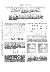
number !:::'(}(Ir, J.l) gives the shift in phase between the two endpoints of the heteroclinic trajectory along the circle of fixed points. In Figs. 7.1 and 7.2 we illustrate the relevant aspects of the geometry and dynamics of the unperturbed system.
Q
x
FIGURE 7.1. The Invariant Manifold Structure of the Unperturbed System.
7.5.2
THE ANALYTIC AND GEOMETRIC STRUCTURE OF THE PERTURBED EQUATIONS
The geometrical structure of the unperturbed system will provide us with the framework for understanding certain types of global behavior that can occur in the perturbed system. In particular, M along with its stable and unstable manifolds will persist in the perturbed system; however, the dynamics on these manifolds will be quite different. This should be evident since M contains a circle of fixed points and the stable and unstable manifolds of M have a coinciding branch; both of these structures are highly degenerate. THE PERSISTENCE OF
M
AND ITS STABLE AND UNSTABLE MANIFOLDS
As we have discussed in Sections 6.3 and 7.2, the problem ofthe persistence of invariant manifolds with boundary under perturbations gives rise to certain technical questions concerning the nature of the trajectories at the boundary. In order to address these questions precisely for this problem, we begin by defining the set
U
6
=
{(x, I, (})
Ilx -
xo(I;J.l)1
~
-
8, It
~
I
~ 12 },
(7.21)
7.5. Invariant Manifold Structure
175
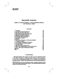
FIGURE 7.2. An Illustration of the Orbits Homoclinic to the Different Invariant Sets in M.
where
h:::; 11 < 12 If h
=
11
and
h
=
12 , then clearly Uti
:::;
h
is the closure of a neighborhood of
M. However, in order to modify the vector field at the boundary to make it
overflowing or inflowing invariant, we will need to slightly restrict the range of 1 values in discussing the perturbed manifolds and it is for this reason that the 1 interval in the definition of Uti has been restricted. (Note: 11 can be chosen arbitrarily close to hand 12 can be chosen arbitrarily close to 12') The set Uti will be useful in characterizing the nature of trajectories near the invariant manifolds. For the unperturbed system, we define the local stable and unstable manifolds of M as follows:
(7.22) (7.23) We now state a persistence theorem which is a restatement of Theorems 3.3.1 and 4.5.1, combined with our discussions in Sections 6.1, 6.3, and 6.4.
176
7. Examples
Theorem 7.5.1 There exists EO > 0 sufficiently small such that for 0 < E ::; EO, M persists as a CT, locally invariant, two-dimensional, normally hyperbolic manifold with boundary, which we denote by M" having the following properties: 1. Me is CT in
E
and 1-".
2. Me is CT E-close to M and can be represented as a graph over M as
(7.24) Moreover, there exists 80 sufficiently small (depending on E) such that for 0 < 8 < 80 there exists locally invariant manifolds in Uti, denoted WI~c(ME)' WI~c(Me), having the following properties:
3. WI~c(ME) and WI~c(ME) are CT in
4·
Wj~C(ME)
n WI~c(Me)
E
and 1-".
= ME'
5. WI~AMe) (resp. WI~AME)) is a graph over WI~c(M) (resp. WI~c(M)) and is CT E-close to WI~c(M) (resp. WI~AM)). 6. Let y:(t) == (x:(t),I:(t),(}:(t)) (resp. y:(t) == (x~(t),I:(t),(}:(t))) denote a trajectory that is in WI~c(Me) (resp. WI~c(ME)) at t = O. Then as t ---t +00 (resp. t ---t -00) either
(a) y:(t) == (x: (t),I: (t), (}:(t)) (resp. y:(t) == (x~(t),I:(t), (}:(t))) crosses au li or (b) limt--+ood(y:(t),ME) = 0 (resp. limt--+-ood(y:(t),Me) = 0), where d(·, .) denotes the standard metric in the phase space. We refer to WI~c(Me) and WI~c(Me) as the local stable and unstable manifolds of Me, respectively.
We make the following remarks concerning the consequences and implications of this theorem. Remark 1. The term locally invariant means that trajectories with initial conditions on ME may leave Me; however, they may do so only by crossing the boundary of ME' In proving the persistence of M under perturbation it is necessary to know the stability properties of trajectories in M on semi-infinite time intervals. Technically, this control
7.5. Invariant Manifold Structure
177
is accomplished by modifying the unperturbed vector field (7.13) in an arbitrarily small neighborhood of the boundary of M by using Coo "bump functions"; this procedure is explained in Wiggins [1988] and in Section 6.3. The perturbed manifold is then constructed as a graph over the unperturbed manifold by using the graph transform technique. This is the reason why the range of I values for which M€ exists in the perturbed vector field (7.13) may need to be slightly decreased. Remark 2. We define the global stable and unstable manifolds of M€, denoted WS(M€) and WU(M€), respectively, as follows. Let 't,
for all t > 0 and for some C, A > 0 as long as (h(t),{J(t)) E A. In other words, trajectories starting on a stable fiber asymptotically approach the trajectory in AE that starts on the basepoint of the same fiber, as long as the trajectory through this basepoint remains in A E • 5. The family of fibers form an invariant family in the sense that fibers map to fibers under the time-T flow map. Analytically, this is expressed as follows. Suppose (Xl (t), X2(t), h(t), O(t)) is a trajectory satisfying X2(0) = X2(Xl(0); Ii, (J, /-L, y'E), h(O) = h(xl(O); Ii, (J, /-L, y'E),
(7.45)
0(0) = O(Xl (0); Ii, (J, /-L, y'E); then X2(t) = X2(Xl (t); Ii(t) , (J(t) , /-L, y'E), h(t) = h(xl (t); h(t), (J(t) , /-L, y'E), O(t)
=
(7.46)
O(Xl(t); Ii(t) , B(t), /-L, y'E).
6. At E = 0 the unperturbed fibers correspond to the unperturbed heteroclinic orbits. Hence, the perturbed and unperturbed fibers are cr y'Eclose. We make the following remarks concerning this theorem.
Remark 1. An identical result follows for the fibering of WU(AE)' Remark 2. Quasilinear partial differential equations whose solutions are the fibers can be derived. These equations are analogous to those given following Theorem 7.5.1. We will not require these for our calculations; however, the reader can find these equations in Fenichel [1979] where a general geometric singular perturbation theory is developed.
References Abraham, R., Marsden, J. E. [1978] Foundations of Mechanics. Addison-Wesley. Abraham, R. A., Marsden, J. E., and Ratiu, T. S. [1988] Manifolds, Tensor Analysis, and Applications. Second edition. Springer-Verlag: New York, Heidelberg, Berlin. Allen, J. S., R. M. Samelson, and P. A. Newberger [1991] Chaos in a model of forced quasiperiodic flow over topographyan application of Melnikov's method. J. Fluid Mech., 226, 511-547. Arnold, V. 1. [1973] Ordinary Differential Equations. M.LT. Press: Cambridge, MA. Ball, J. [1973] Saddle point analysis for an ordinary differential equation in a Banach space, and an application to dynamic buckling of a beam, in Nonlinear Elasticity (R. W. Dickey, ed.), Academic Press: New York, 93-160. Ball, J. M., Holmes, P. J., James, R. D., Pego, R. L, and Swart, P. J. [1991] On the Dynamics of Fine Structure. J. Nonlinear Sci., 1(1), 17-70. Bates, P. W. and Jones, C. K. R. T. [1989] Invariant Manifolds for Semilinear Partial Differential Equations. Dynamics Reported, 2, 1-38. Benedicks, M. and Carleson, L. [1991] The Dynamics of the Henon Map. Annals of Math., 133(1), 73-170. Benettin, G., Galgani, L., Giorgilli, A., and Strelcyn, J.-M. [1984] A proof of Kolmogorov's theorem on invariant tori using canonical transformations defined by the Lie method. Nuovo Cimento B, 79(2), 201-223. Berger, M. and Gostiaux, B. [1988] Differential Geometry: Manifolds, Curves, and Surfaces. Springer-Verlag: New York, Heidelberg, Berlin. Bleher, S., Grebogi, C., and Ott, E. [1990] Bifurcation to Chaotic Scattering. Physica D, 46, 87-121.
186
References
Bruhn, B. and Koch, B. P. [1991] Heteroclinic bifurcations and invariant manifolds in rocking block dynamics. Z. Naturforsch., 46a, 481-490. Chow, S. N. and Hale, J. K. [1982] Methods of Bifurcation Theory. Springer-Verlag: New York, Heidelberg, Berlin. Constantin, P., Foias, C., Nicolaenko, B., and Temam, R. [1989] Integral Manifolds and Inertial Manifolds for Dissipative Partial Differential Equations. Springer-Verlag: New York, Heidelberg, Berlin. Coppel, W. A. [1978] Dichotomies in Stability Theory. Lecture Notes in Mathematics, Vol. 629. Springer-Verlag: New York, Heidelberg, Berlin. Davis, M. J. [1987] Phase space dynamics of bimolecular reactions and the breakdown of transition state theory. J. Chem. Phys., 86(7), 3978-4003. de la Llave, R. and Wayne, C. E. [1993] On Irwin's proof of the pseudostable manifold theorem. Univ. of Texas preprint. Dieudonne, J. [1960] Foundations of Modern Analysis. Academic Press: New York. Falzarano, J., Shaw, S. W., and Troesch, A. W. [1992] Applications of global methods for analyzing dynamical systems to ship rolling motion and capsizing. International J. of Bifurcations and Chaos, 21, 101-115. Fenichel, N. [1970] Ph. D. Thesis, New York University. Fenichel, N. [1971] Persistence and smoothness of invariant manifolds for flows. Ind. Univ. Math. J., 21, 193-225. Fenichel, N. [1974] Asymptotic stability with rate conditions. Ind. Univ. Math. J., 23, 1109--1137. Fenichel, N. [1977] Asymptotic stability with rate conditions, II. Ind. Univ. Math. J., 26, 81-93. Fenichel, N. [1979] Geometric singular perturbation theory for ordinary differential equations. J. Diff. Eqns., 31, 53-98. Fuks, D. B. and Rokhlin, V. A. [1984] Beginner's Course in Topology: Geometric Chapters. Springer-Verlag: New York, Heidelberg, Berlin. Gillilan, R. and Ezra, G. S. [1991] Transport and turnstiles in multidimensional Hamiltonian mappings for unimolecular fragmentation: application to van der Waals predissociation. J. Chem. Phys., 94(4), 2648-2668.
References Guillemin, V. and Pollack, A. [1974] Differential Topology. Prentice Hall, Inc.: Englewood Cliffs, NJ. Hadamard, J. [1901]. Sur l'iteration et les solutions asymptotiques des equations differentielles. Bull. Soc. Math. France, 29, 224~228. Hale, J. [1980] Ordinary Differential Equations. Robert E. Krieger Publishing Co., Inc.: Malabar, Florida. Haller, G. and Wiggins, S. [1992] Whiskered tori and chaos in resonant Hamiltonian normal forms. Accepted for publication in the proceedings of the workshop on Normal Forms and Homoclinic Chaos. The Fields Institute: Waterloo, Ontario. Haller, G. and Wiggins, S. [1993a] Orbits homo clinic to resonances: The Hamiltonian case. Physica D, 66, 298~346. Haller, G. and Wiggins, S. [1993b] N-Pulse homoclinic orbits in perturbations of hyperbolic manifolds of Hamiltonian equilibria. submitted to Arch. Rat. Mech. Anal.. Henry, D. [1981]. Geometric Theory of Semilinear Parabolic Equations. Springer Lecture Notes in Mathematics Vol. 840. Springer-Verlag: New York, Heidelberg, Berlin. Hirsch, M.W., Pugh, C.C., and Shub, M. [1977] Invariant Manifolds, Lecture Notes in Mathematics Vol. 583. SpringerVerlag: New York, Heidelberg, Berlin. Hirsch, M. W. and Smale, S. [1974] Differential Equations, Dynamical Systems, and Linear Algebra. Academic Press: New York. Hoveijn, 1. [1992] Aspects of Resonance in Dynamical Systems. Ph.D. thesis, University of Utrecht. Irwin, M. C. [1970] On the stable manifold theorem. Bull. London Math. Soc., 2, 196~198. Irwin, M. C. [1980] A new proof of the pseudostable manifold theorem. Jour. London Math. Soc., 21, 557~566. Kang, 1. S. and Leal, L. G. [1990] Bubble dynamics in timeperiodic straining flows. J. Fluid Mech., 218, 41~69. Kirchgraber, U. and Palmer, K. J. [1990] Geometry in the Neighborhood of Invariant Manifolds of Maps and Flows and Linearization. Pitman Research Notes in Mathematics Series. Longman Scientific & Technical. Published in the United States with John Wiley & Sons, Inc.: New York.
187
188
References Kopell, N. [1979] A geometric approach to boundary layer problems exhibiting resonance. SIAM J. Appl. Math., 37(2), 436-458. Kopell, N. [1985] Invariant manifolds and the initialization problem for some atmospheric equations. Physica D, 14, 203-215. KovaCic, G. and Wiggins, S. [1992] Orbits homoclinic to resonances, with an application to chaos in a model of the forced and damped sine-Gordon equation, Physica D, 57, 185-225. Liapunov, A. M. [1947] Probleme general de la stabilite du movement. Princeton University Press: Princeton. Lin, X.-B. [1989] Shadowing lemma and singularly perturbed boundary value problems. SIAM J. Appl. Math., 49(1), 2654. Llavona, J. G. [1986] Approximation of Continuously Differentiable Functions. North-Holland: Amsterdam. Lochak, P. [1992] Canonical perturbation theory via simultaneous approximation. Russian Math. Surveys, 47(6), 57-133. Marsden, J. E. and Scheurle, J. [1987] The construction and smoothness of invariant manifolds by the deformation method. SIAM J. Math. Anal., 18(5), 1261-1274. McLaughlin, D., Overman II, E.A., Wiggins, S., and Xiong, X. [1993] Homoclinic orbits in a four dimensional model of a perturbed NLS equation: A geometric singular perturbation study. submitted to Dynamics Reported. Milnor, J. W. [1965] Topology from the Differentiable Viewpoint. University of Virginia Press: Charlottesville. Nijmeijer, H. and van der Schaft, A. J. [1990] Nonlinear dynamical control systems. Springer-Verlag: New York, Heidelberg, Berlin. Odyniec, M. and Chua, L. [1983] Josephson-junction circuit analysis via integral manifolds. IEEE Trans. on Cire. and Systems, cas-30(5), 308-320. Odyniec, M. and Chua, L. [1985] Josephson-junction circuit analysis via integral manifolds. IEEE Trans. on Circ. and Systems, cas-32(1), 34-45. Ottino, J.M. [1989] The Kinematics of Mixing: Stretching, Chaos and Transport. Cambridge University Press: Cambridge.
References Palis, J. and Takens, F. [1993] Hyperbolicity fj Sensitive Chaotic Dynamics at Homoclinic Bifurcations. Cambridge University Press: Cambridge. Perron, O. [1928]. Uber stabilitat und asymptotisches verhalten der integrale von differentialgleichungssystem. Math. Z., 29, 129-160. Perron, O. [1929] Uber stabilitat und asymptotisches verhalten der losungen eines systems endlicher differenzengleichungen. J. Reine Angew. Math., 161, 41-64. Perron, O. [1930] Die stabilitatsfrage bei differentialgleichungen. Math. Z., 1930, 703-728. Petschel, G. and Geisel, T. [1991] Unusual manifold structure and anomalous diffusion in a Hamiltonian model for chaotic guiding center motion. Physical Review A, 44(12), 79597967. Poschel, J. [1993] Nekhoroshev estimates for quasi-convex Hamiltonian systems. Mathematische Zeitschrijt, 213(2), 187-216. Rudin, W. [1964] Principles of Mathematical Analysis. McGraw-Hill: New York. Sacker, R. J. [1969] A perturbation theorem for invariant manifolds and Holder continuity. J. Math. Mech., 18, 187-198. Sacker, R. J. and Sell, G. R. [1974] Existence of dichotomies and invariant splittings for linear differential systems. J. Diff. Eqns., 15, 429-458. Silnikov, L. P. [1967] On a Poincare-Birkhoff problem. Math. USSR Sb., 3, 353-371. Spivak, M. [1979] Differential Geometry, Vol. I. Second edition. Publish or Perish, Inc.: Wilmington, DE. Temam, R. [1988] Infinite Dimensional Dynamical Systems in Mechanics and Physics. Springer-Verlag: New York, Heidelberg, Berlin. Terman, D. [1992] The Transition form Bursting to Continuous Spiking in Excitable Membrane Models. J. Nonlinear Sci.,2(2), 135-182. Touma, J. and Wisdom, J. [1993] The Chaotic Obliquity of Mars. Science, 259, 1294-1297. Wagenhuber, J., Geisel, T., Niebauer, P., and Obermair, G. [1992] Chaos and anomalous diffusion of ballistic electrons in lateral surface superlattices. Physical Review B, 45(8), 4372-4383.
189
190
References Wells, J. C. [1976J Invariant Manifolds of non-linear operators. Pac. Jour. Math., 62, 285~293. Whitney, H. [1936J Differentiable Manifolds. Ann. Math., 37(3), 645~680.
Wiggins, S. [1988J Global Bifurcations and Chaos ~ Analytical Methods. Springer-Verlag: New York, Heidelberg, Berlin. Wiggins, S. [1990J On the geometry of transport in phase space, 1. 'fransport in k-degree-of-freedom Hamiltonian systems, 2 :::; k < 00, Physica D, 44, 471~501. Wiggins, S. [1992J Chaotic Transport in Dynamical Systems. Springer-Verlag: New York, Heidelberg, Berlin. Yi, y. [1993aJ A generalized integral manifold thorem. J. DijJ. Eq., 102(1), 153~187. Yi, Y. [1993bJ Stability of integral manifold and orbital attraction of quasiperiodic motion. J. DijJ. Eq., 103(2), 278~322.
Index A
D
atlas, 23 atlas for M, 34 atlas for T M, 34
derivative, 29 derivative of a map, 21 derivative of maps between manifolds, 32 derivative of the section, 92 differentiable, 28 differentiable manifold, 22 direct sum, 34, 47
B basepoint of the fiber, 35, 47 base space of the vector bundle, 119 boundary of M, 40
c cr
bundle transverse to TM1 , 72 C r diffeomorphism, 22 CO topology, 55 C r - 1 orthonormal basis, 70, 71 center manifold, 167 change of coordinates, 24 chart, 23 closed half-space, 40 compact, boundaryless invariant manifolds, 159 continuous splitting, 111 contraction mapping theorem, 53 contractive property, 76 coordinate charts, 70 curve, 29
E
Euclidean inner product, 33 Euclidean spaces, 22
F fiber, 35, 45 fiber projection map, 35, 82 finite cylinder, 40 G
generalized Lyapunov-type numbers, 58, 111, 166 geometric singular perturbation theory, 183 global perturbation methods, 1, 41,171
192
Index
graph of a section, 119 graph transform, 81 Gronwall estimate, 76 Gronwall's inequality, 79 H Hamiltonian perturbations, 171 higher order derivatives, 101 I identity operator, 95 inflowing invariant, 51 inflowing invariant manifold, 159 invariant, 51 invariant set, 42 inverse function theorem, 36 L linear structure, 29 local parametrization of N, 47 local triviality, 70 local triviality of the normal bundIe, 37 locally invariant, 52
o open covers, 70 orthogonal bundle projection map, 35 orthogonal complement, 45 orthogonal projection map, 35, 47 orthogonal projection operator, 57 overflowing invariant, 51 overflowing invariant ellipsoid, 166 overflowing invariant manifold(s), 159, 165 overflowing invariant Lipschitz manifold, 92
p partition(s) of unity, 36, 94 persistence theorem, 85, 166, 176 projection map, 22 projections, 111
Q quasilinear partial differential equations, 183
R M manifold with boundary, 40 matrix representation, 47
resonant fixed points, 173 resonant I value, 173
s N
neighborhood of M, 114 neighborhood of M, 48 neighborhood of a manifold, 36 neighborhood of the zero section, 73 non-Hamiltonian perturbations, 171 normal bundle, 34, 36, 45 normal space at a point, 33
section, 35 section of N' € over N'~, 119 singular perturbation, 182 space of sections, 81 stable and unstable manifold theorem for a hyperbolic fixed point, 165 standard inner product, 45 standard metric, 45
Index
sterographic projections, 41 subbundles, 111 symplectic matrix, 171 T
tangent bundle, 34 tangent space at a point, 28-30 tangent vector at a point, 29 Taylor expansion methods, 170 time reversal, 159 time-reversed vector field, 166 two-degree-of-freedom Hamiltonian systems, 171 two-dimensional sphere, 26 two-sphere, 37
w weak hyperbolicity, 168 Whitney sum, 35, 47
z zero section, 35
Symbols
11, 95 A t (p),57 Bt(p), 57 MI ,56 M 2 ,56
u uniformity lemma, 65, 113 unstable manifold, 111, 119 unstable manifold theorem, 120
v vector bundle over N'~, 119 vector bundles, 35
N;,73 lI(p), 58-59 a(p),59 ai,70 ai x Ti, 74 Ti,73 U/,70 X(p),82 w,82
193
Applied Mathematical Sciences (continued from page ii) 52. 53. 54. 55. 56. 57. 58. 59. 60. 61. 62. 63. 64. 65. 66. 67. 68. 69. 70. 71. 72. 73. 74. 75. 76. 77. 78. 79. 80. 81. 82. 83. 84. 85. 86. 87. 88. 89.
90. 91. 92. 93. 94. 95. 96. 97. 98. 99. 100. 101. 102. 103. 104. 105.
Chipot: Variational Inequalities and Flow in Porous Media. Majda: Compressible Fluid Flow and System of Conservation Laws in Several Space Variables. Wasow: Linear Turning Point Theory. Yosida: Operational Calculus: A Theory of Hyperfunctions. Chang/Howes: Nonlinear Singular Perturbation Phenomena: Theory and Applications. Reinhardt: Analysis of Approximation Methods for Differential and Integral Equations. Dwoyer/HussainWoigt (eds): Theoretical Approaches to Turbulence. Sanders/Verhulst: Averaging Methods in Nonlinear Dynamical Systems. GhillChildress: Topics in Geophysical Dynamics: Atmospheric Dynamics, Dynamo Theory and Climate Dynamics. SattingerlWeaver: Lie Groups and Algebra~ with Applications to Physics, Geometry, and Mechanics. LaSalle: The Stability and Control of Discrete Processes. Grasman: Asymptotic Methods of Relaxation Oscillations and Applications. Hsu: Cell-to-Cell Mapping: A Method of Global Analysis for Nonlinear Systems. Rand/Armbruster: Perturbation Methods, Bifurcation Theory and Computer Algebra. HlavaceklHaslingerlNecasllLavIsek: Solution of Variational Inequalities in Mechanics. Cercignani: The Boltzmann Equation and Its Applications. Temam: Infinite Dimensional Dynamical Systems in Mechanics and Physics. Golubitsky/StewartiSchae!fer: Singularities and Groups in Bifurcation Theory, Vol. ll. Constantin/Foias/Nicolaenko/Temam: Integral Manifolds and Inertial Manifolds for Dissipative Partial Differential Equations. Catlin: Estimation, Control, and the Discrete Kalman Filter. LochakiMeunier: Multiphase Averaging for Classical Systems. Wiggins: Global Bifurcations and Chaos. MawhinIWillem: Critical Point Theory and Hamiltonian Systems. AbrahamlMarsden/Ratiu: Manifolds, Tensor Analysis, and Applications, 2nd ed. Lagerstrom: Matched Asymptotic Expansions: Ideas and Techniques. Aldous: Probability Approximations via the Poisson Clumping Heuristic. Dacorogna: Direct Methods in the Calculus of Variations. Hernandez-Lerma: Adaptive Markov Processes. Lawden: Elliptic Functions and Applications. Bluman/Kumei: Symmetries and Differential Equations. Kress: Linear Integral Equations. Bebernes/Eberly: Mathematical Problems from Combustion Theory. Joseph: Fluid Dynamics of Viscoelastic Fluid~. Yang: Wave Packets and Their Bifurcations in Geophysical Fluid Dynamics. DendrinosiSonis: Chaos and Socio-Spatial Dynamics. Weder: Spectral and Scattering Theory for Wave Propagation in Perturbed Stratified Media. BogaevskilPovzner: Algebraic Methods in Nonlinear Perturbation Theory. O'Malley: Singular Perturbation Methods for Ordinary Differential Equations. Meyer/Hall: Introduction to Hamiltonian Dynamical Systems and the N-body Problem. Straughan: The Energy Method, Stability, and Nonlinear Convection. Naber: The Geometry of Minkowski Spacetime. Colton/Kress: Inverse Acoustic and Electromagnetic Scattering Theory. Hoppensteadt: Analysis and Simulation of Chaotic Systems. Hackbusch: Iterative Solution of Large Sparse Systems of Equations. Marchioro/Pulvirenti: Mathematical Theory of Incompressible Nonviscous Fluids. Lasota/Mackey: Chaos, Fractals, and Noise: Stochastic Aspects of Dynamics, 2nd ed. de Boor/Hollig/Riemenschneider: Box Splines. Hale/Lunel: Introduction to Functional Differential Equations. Sirovich (ed.): Trends and Perspectives in Applied Mathematics. NusseIYorke: Dynamics: Numerical Explorations. Chossatllooss: The Couette-Taylor Problem. Chorin: Vorticity and Turbulence. Farkas: Periodic Motions. Wiggins: Normally Hyperbolic Invariant Manifolds in Dynamical Systems.