Mar 2, 2009 - For three-subscale assessments such as these, CGROUP, the ... for CGROUP than for BGROUP, and all three correlations are slightly lower for ...
Research Report
Stochastic Approximation Methods for Latent Regression Item Response Models
Matthias von Davier Sandip Sinharay
March 2009 ETS RR-09-09
Listening. Learning. Leading.®
Stochastic Approximation Methods for Latent Regression Item Response Models
Matthias von Davier and Sandip Sinharay ETS, Princeton, New Jersey
March 2009
As part of its nonprofit mission, ETS conducts and disseminates the results of research to advance quality and equity in education and assessment for the benefit of ETS’s constituents and the field. To obtain a PDF or a print copy of a report, please visit: http://www.ets.org/research/contact.html
Copyright © 2009 by Educational Testing Service. All rights reserved. ETS, the ETS logo, and LISTENING. LEARNING. LEADING. are registered trademarks of Educational Testing Service (ETS).
Abstract This paper presents an application of a stochastic approximation EM-algorithm using a Metropolis-Hastings sampler to estimate the parameters of an item response latent regression model. Latent regression models are extensions of item response theory (IRT) to a 2-level latent variable model in which covariates serve as predictors of the conditional distribution of ability. Applications for estimating latent regression models for data from the 2000 National Assessment of Educational Progress (NAEP) grade 4 math assessment and the 2002 grade 8 reading assessment are presented and results of the proposed method are compared to results obtained using current operational procedures.
Key words: Conditioning, IRT, NAEP, latent regression
i
1
Introduction
Item response theory (IRT; Lord & Novick, 1968) is the method of choice for assessment designs involving multiple test forms that require linking in order to compare individuals or groups based on the same variables. Standard examples of such assessment designs are educational survey assessments such as the National Assessment of Educational Progress (NAEP), the Programme for International Student Assessment (PISA), and the Trends in International Mathematics and Science Study (TIMSS), and the Progress in International Reading Literacy Study (PIRLS), to name a few. In these assessments, every examinee responds to one out of many test booklets addressing the same content domain(s) with different, but overlapping subsets of items. The testing time in these assessments is short, since the results obtained are inconsequential for the participants. Therefore, in order to cover the proficiency domain sufficiently, multiple booklets are used, each of which contains a small subset of the total number of items. This design feature allows several hundreds of items to be covered, while each student is tested for only about 60–90 minutes. Several extensions of IRT have been developed for supplementing the relatively sparse information obtained from the short booklets used in educational survey assessments. Many of these developments follow original ideas by Mislevy (1984). von Davier, Sinharay, Oranje, and Beaton (2006) described recent developments and operational procedures used in NAEP. The major extension to IRT used in these methods is based on the need for estimating unbiased group-level distributions of proficiency for policy-relevant subpopulations (such as gender groups) and groups defined by self-reported ethnicity. These extensions of IRT make use of the fact that a large number of background variables (such as gender, ethnicity, and socio-economic variables) are collected as covariates of the proficiency variables during the survey. Examinees are asked to respond to a questionnaire section containing questions on these and other variables, such as attitudes toward content domains like physics, mathematics, or reading (depending on what is assessed in the test), as well as study skills, and other covariates. These covariates are used in a latent regression model that extends IRT to a two-level latent variable model in which the background 1
variables serve as predictors of the conditional distribution of ability. In addition to the presence of a (potentially large) number of covariates, survey assessments often contain multiple subscales of the content domain of interest. These subscales are designed in such a way that each item in the survey is assumed to measure only one scale, so that the set of items measuring the k content (subdomains) can be treated as a k-scale simple-structure multidimensional IRT (MIRT) model. The correlations between subscales are included in the model by means of extending the latent regression to a multivariate, multiple latent regression, in which the conditional mean vector of proficiencies (subscales) is predicted by the set of covariates, while the conditional covariance matrix of proficiencies is assumed to be the same for all subpopulations (see Thomas, 2002, and von Davier et al., 2006, for models relaxing these assumptions). This multivariate multiple latent regression model requires the evaluation or approximation of multidimensional integrals, a task that in past decades required days on working on computers if large numbers of covariates were used. Additionally, the dimension is k > 3. Research has attempted to reduce the computational burden either by using approximations (Thomas, 1993; von Davier, 2003) or by using stochastic methods (Adams, Wilson, & Wu, 1997; von Davier & Sinharay, 2007). Neither of these approaches is completely satisfactory. They either rely on strong assumptions about the shape of the functions involved, or they use stochastic methods that do not rely on strong assumptions and do not deliver the promised increase in speed (at least when using simulation sample sizes to provide sufficient accuracy). This paper explores an alternative to the methods used so far for multivariate latent regressions and presents an application of a stochastic approximation EM-algorithm using a Metropolis-Hastings (MH) sampler (Cai, 2007; Delyon, Lavielle, & Moulines, 1999; Gu & Kong, 1998; Gu & Zhu, 2001) to estimate the parameters of an item response latent regression model. Applications for estimating latent regression models for NAEP data from the 2000 grade 4 math assessment and the 2002 grade 8 reading assessment are presented, and results of the proposed method are compared to results obtained using current operational procedures.
2
2
Item Response Latent Regression Models
Assume Y1, , . . . , YI categorical observed random variables and X1 , . . . , XK real valued random variables, with realizations on these variables sampled from N examinees. Let (yv , xv ) = (yv1 , . . . , yvi , xv1 , . . . , xvK ) denote the realizations for examinee v. Let (θ1 , . . . , θd ) be a d-dimensional real number representing the ability variable, and let P (y | θ) =
I Y
Pi (yi | θ)
i=1
be a model describing the probability of the observed categorical variables given the d-dimensional parameter θ, referred to as proficiency variable in the subsequent text. For these product terms, assume that Pi (y | θ) = P (y | θ; ζi ) with some vector-valued parameter ζi . Examples are unidimensional item response models, such as Pi (y | θ1 , . . . , θd ) =
exp(ya θ − biy ) Pmi i j , 1 + z=1 exp(zai θj − biz )
where the probability depends on one component, θj . Similar models suitable for generating multinomial probabilities for (mi + 1)-categorical variables can also be considered. For the proficiency variable θ = (θ1 , . . . , θd ), assume that
θv ∼ N (xv Γ, Σ), with d × d-variance-covariance matrix Σ and K-dimensional regression parameter Γ. Let φ(θ; | xv Γ, Σ) denote the multivariate normal density with mean xv Γ and covariance matrix Σ. Then, the likelihood of an observation (yv , xv ) expressed as a function of ζ, Γ, and Σ can be written as Z Y I L(ζ, Γ, Σ; yv , xv ) = ( P (yvi | θ; ζ))φ(θ | xv Γ, Σ)dθ, θ i=1
and, for the log-likelihood function involving all N examinees, we have log L(ζ, Γ, Σ; Y, X) =
N X
I Y log intθ ( P (yvi | θ; ζ))φ(θ | xv Γ, Σ)dθ.
v=1
i=1
3
(1)
This log-likelihood function is the objective function to be maximized with respect to parameters Σ, Γ, and ζ. Current Operational Estimation Procedures In NAEP operational analyses, the item parameters ζ associated with the
Q
i
P (yi | θ; ζ)
are often determined in a separate estimation phase prior to the estimation of the latent regression φ(θ | xv Γ, Σ). In the second phase, the latent regression parameters Σ and Γ ˆ These item parameters are estimated using the previously determined item estimates of ζ. are plugged into the second phase as fixed and known constants. von Davier et al. (2006) described this procedure, which is the current method of choice in analysis of many national and international large-scale survey assessments, including NAEP, TIMSS, PIRLS, and PISA. The evaluation of the likelihood function in (1) requires the calculation or approximation of multidimensional integrals over the range of θ. The evaluation of these integrals is quite time-consuming for integrals with dimension d > 5. Even if adaptive numerical integration methods are used, the time required per integral increases with the number of dimensions, and the integration has to be repeated N times in each step of the estimation. Mislevy, Beaton, Kaplan, and Sheehan (1992) suggested use of the EM-algorithm (Dempster, Laird, & Rubin, 1977) for maximization of L in (1) with respect to Γand Σ. The EM-algorithm treats estimation problems with latent variables as an incomplete data problem and completes the required statistics in one phase (the E-step, where E stands for expectation), and then maximizes the resulting complete-data likelihood with respect to the parameters of interest (the M-step, where M stands for maximization). In the case of the latent regression, the EM-algorithm operates as follows: E-step: The integral over the unobserved latent variable θ is evaluated in the (t)-th E-step using the provisional estimates Σ(t) and Γ(t) . As in the previous section, let P (yvi | θ; ζi ) denote the probability of response yvi , given ability θ and item
4
parameters ζi . Then we have Z Y I ( P (yvi | θ; ζ))φ(θ | xv Γ(t) , Σ(t) )dθ. θ i=1 (t) Let the posterior mean of θ be denoted by θ˜v = E(Σ,Γ,ζ)(t) (θ | yv , xv ). Mislevy et al.
(1992) argued that the posterior mean θ˜v can subsequently be plugged into the ordinary least squares (OLS) estimation equations. Note that the calculation of the θ˜(t) also requires the evaluation or approximation of an integral, since calculation of the expectation Z E(Σ,Γ,ζ)(t) (θ | yv , xv ) = θ
I Y θ( P (yvi | θ; ζ))φ(θ | φ(xv Γ(t) , Σ(t) )dθ i=1
is involved. M-step: Following the arguments put forward by Mislevy et al. (1992), the maximization of the likelihood for step (t + 1) based on provisional estimates from the preceding E-step is accomplished by using OLS estimation equations with the posterior means generated in the E-step, as outlined in the previous paragraphs. This yields ˜ (t+1) = (XT X)−1 XT θ˜(t) . Γ An estimate of the conditional variance-covariance matrix is given by Σ(t+1) = V (θ˜ − XΓ(t+1) ) + E(V(Σ,Γ,ζ)(t) (θ | yv , xv )). The computationally intensive calculations involved here are the determination of estimates or approximations of E(Σ,Γ,ζ)(t) (θ | yv , xv ) and V(Σ,Γ,ζ)(t) (θ | yv , xv ) for each of the N observations; both calculations involve the numerical evaluation or the approximation of (multidimensional) integrals. If the dimension d is large (d > 4 in this context), this evaluation can be rather time-consuming. 3
Metropolis-Hastings Stochastic Approximation
Maximum-likelihood estimation for likelihood functions that involve a large number of random effects or latent variables can be very time consuming due to the need to 5
evaluate integrals in multiple dimensions. Researchers have examined stochastic versions of numerical integration methods as potential alternatives that allow estimation of high-dimensional models in shorter time. Von Davier and Sinharay (2007) employed importance sampling in a stochastic EM-algorithm for estimating the parameters of a latent regression with a multidimensional IRT measurement model. Adams et al. (1997) used stochastic methods to evaluate integrals for the estimation of multidimensional generalized Rasch models. Gu and Kong (1998) demonstrated the use of stochastic approximation with a Markov-chain generated by an MH sampler, as did Delyon et al. (1999) for the EM-algorithm. Gu and Zhu (2001) as well as Kuhn and Lavielle (2004) showed how to combine Markov chain Monte Carlo (MCMC) and stochastic approximation. To our knowledge, stochastic approximation has never been applied to large-scale data analysis with latent regression models involving hundreds of parameters estimated based on samples composed of some 10,000 to 100,000 observations. The rationale behind the proposed MH stochastic approximation makes this an area where this method is likely to prove useful. Stochastic Approximation for Optimization Stochastic approximation methods are often introduced to solve the following problem. Assume that there is a function L(α | z, η) with α being the parameters to be maximized, and observed data z, while the η are not directly observable quantities. Assume that L(α | z, η) is difficult to calculate due to the latency of η, for example, while there is a proxy to this function, L∗ (α | x, ζ), which can be calculated easily. Assume that L(α | z, η) = L∗ (α | z, ζ) + �, with � small. The proxy L∗ could be viewed as a noisy version of L. If the task is to find an extreme value of L with respect to parameter α, one might choose to employ either gradient descent methods or Newton-Raphson methods, since in most cases there is no analytic solution at hand. For gradient descent methods, we have α(t+1) = α(t) + λt ∇L(α(t) | z, η),
6
with some efficient algorithm to determine the step-width λt for each cycle (t) of the iterative algorithm. The iterations implied in this discussion are continued until convergence is reached, which is often determined by the sequence α(t+1) not changing by more than a constant ε. Obviously, this may be the case once λt reaches some value smaller than cε for some constant c. In order to avoid computationally costly evaluations of L(α | z, η), stochastic approximation methods instead use the noisy replacement L∗ (α | z, ζ). Alternatively, a noisy replacement of the gradient is used, that is,
∇L∗ (α | z, ζ) = (
δ ∗ δ ∗ L (α | z, ζ), . . . , L (α | z, ζ)), δα1 δαK
so that the updated rule becomes α(t+1) = α(t) + δt ∇L∗ (α(t) | z, ζ), with some step-width δt , for which
P
t δt
= ∞ and
2 t δt
P
< ∞ holds. Often δt = 1/t is used.
In the case considered here, the function L is the likelihood function used to estimate the parameters of a latent regression. A regression is termed latent regression when the dependent variable is unobserved and has to be replaced by a conditional expectation for each observation v. The proxy of this likelihood function, L∗ , is an estimator of the same regression, for example, where the dependent variable is unobserved but values are plugged in from the conditional distribution of the dependent variable rather than from an estimate of the conditional expectation. In other words, instead of plugging in an estimate of θ˜ = E(θ | z), we use a draw θˆ from the posterior ∼ P (θ | z) as the plug-in for the estimator (XT X)−1 Xθ. The Metropolis-Hastings (MH-) Algorithm The MH-algorithm (Gelman, Carlin, Stern, & Rubin, 1995; Hastings, 1970; Metropolis, Rosenbluth, Rosenbluth, Teller, & Teller, 1953) is a method to generate a Markov chain of draws from a distribution p(θ | z) without the need for calculating the density as a whole or to approximate it. It is sufficient to be able to calculate values proportional to p(θ∗ | z) for 7
a sequence of values of θ∗ drawn from some jump distribution fθnew |θold (θnew ) = q(θold , θnew ). The jump distribution q(θold , θnew ) defines a conditional distribution of the new value θnew given the previous value θold . Then the MH-algorithm operates as follows: • First, some initial value θ0 is drawn from q(0, θ0 ) and the old, or previous, value θold is established. • Second, a new proposed value θnew is generated using q(θold , θnew ). • Third, it is determined whether this new θnew should be accepted, using the ratio r=
p(θnew | z)q(θnew , θold ) p(θold | z)q(θold , θnew )
with acceptance rate P (θn | θ0 ) = min(1, r). The calculation of P (θ | z) often involves expressions of the form p(θ | z) = R
p(z | θ)P (θ) p(z | θ)P (θ)dθ θ
so that the calculation of the ratio r turns out to reduce to a simple expression p(z | θnew )p(θnew )q(θnew , θold ) r= , p(z | θold )p(θold )q(θold , θnew ) which is often easy to calculate. 4
Application to NAEP Latent Regression
It is proposed to estimate the latent regression, which is the population model θ = xΓ+� using stochastic approximation by means of an MH sampler, with the commonly employed monotone decreasing sequence of weights, or step-widths, δt = 1t . More specifically, we define a process that produces draws from the posterior distribution of θ, given observations yv and covariates xv , using the provisional estimates of Σ(t) and Γ(t) . More specifically, the algorithm proposed here will provide draws from the posterior θˆv(t) ∼ P(Σ,Γ,ζ)(t) (θ | yv , xv ) and will base the iterative updating of the estimates Σ(t) and Γ(t) on principles of a decreasing sequence of weights δt as outlined in Gu and Kong (1998) and Cai (2007). 8
(2)
Metropolis-Hastings Process for Latent Regressions Following Gu and Kong (1998) and Cai (2007), we propose to use the MH-algorithm for generating draws from the posterior given in (2). A yet to be determined function of these draws from the posterior distribution will serve as a noisy estimate of the posterior mean required in the EM-algorithm for estimating latent regressions. The posterior probability of the d-dimensional ability variable θ given responses y and covariates x is
P (θ | yv , xv ) = R
P (yv | θ)P (θ | xv ) , P (y | θ)P (θ | x )dθ v v θ
with multivariate normal density P (θ | xv ) = φ(θ | xv Γ, Σ), covariance matrix Σ, and conditional mean xv Γ. For the jump distribution in iteration (t), we choose θn ∼ N (θo , cΣ(t) ), that is q(θold , θnew ) = φ(θnew | θold , cΣ(t) ) with some constant c (Gelman et al., 1995). Then, the ratio r used to determine the acceptance probability for the next draw in the MH chain is given by r=
P (yv | θnew )P (θnew | xv ) , P (yv | θold )P (θold | xv )
since q() = φ() is symmetric. The acceptance probability is defined as presented in this discussion and equals P (θnew | θold ) = min(r, 1). This produces a series of draws from P (t) (θ | yv , xv ) ∼ P (yv | θ)φ(xv Γ(t) , Σ(t) ). Note that there are two terms involved in these calculations that depend on estimates obtained in cycle (t). More specifically, the actual use of q(θold , θnew ) in cycle (t) requires plugging in the current estimate of the conditional covariance matrix, that is q (t) (θold , θnew ) = φ(θnew | θold , Σ(t) ). In addition, the conditional distribution depends on the estimates obtained in cycle (t) as P (t) (θ | xv ) = φ(θ | xv Γ(t) , Σ(t) ).
9
Updating Regression Parameters Γ(t+1) and Σ(t+1) Using Stochastic Approximation The principle behind stochastic approximation methods is a combination of evaluating noisy versions of the objective function and defining a sequence of updates that use decreasing weights so that the impact of using noisy functions is averaged out over the course of the optimization process. However, the determination of the latent regression parameters following the methods put forward by Mislevy et al. (1992) is conducted as a one-step estimator, calculated in each M-step of their proposed EM-algorithm. Plugging in the noisy estimate θˆ(t) directly would yield ˜ (t+1) = (XT X)−1 XT θˆ(t) . Γ This one-step estimator produces a noisy estimate of the current state of affairs in the EM-algorithm. Therefore, following the principle put forward by Robbins and Monro (1951), the change in estimates due to noisiness needs to be tempered by defining a weighted average of the current and previous states of the iterations. For a regression estimator, this can be done by exploiting the fact that the OLS estimator is linear in the dependent variable. Define the difference (t) θd = (θˆ(t) − θˆ(t−1) ),
and calculate the regression parameter based on this vector of differences of the unobserved target of inference between the previous cycle (t − 1) and the current cycle (t), ˜ (t+1) = (XT X)−1 XT θˆ(t) . Γ d d Then, calculate the update using the weight δt , ˜ (t+1) . ˆ (t+1) = Γ ˆ (t) + δt+1 Γ Γ d ˜ based This update of the previous estimate Γ(t) by means of the weighted estimator δt+1 Γ on the change (or difference), θˆ(t) − θˆ(t−1) , is equivalent to ˜ (t+1) ˆ (t+1) = (1 − δt+1 )Γ ˆ (t) + δt+1 Γ Γ 10
ˆ (0) = 0, due to linearity of the OLS estimator. The sequence of updates can be started using Γ ˆ (0) , Γ ˆ (1) , . . . , Γ ˆ (t) , Γ ˆ (t+1) , . . . , since δ1 = 1; therefore, (1 − δ1 ) = 0. This yields a sequence Γ ˆ (t) being determined recursively by the previous estimates with each instance of the Γ Γ(0) . . . Γ(t−1) and updated with a weight of δt = 1/t to account for the current noisy, but improved, approximation of the system. Similarly, define ˆ (t+1) = (1 − δt+1 )Σ ˆ (t) + δt+1 Σ ˜ (t+1) , Σ with ˜ (t+1) = V (θˆ − XΓ ˆ (t+1) ). Σ The main challenge of the proposed method will be evaluating and determining convergence, since the decreasing weights δt enforce diminishing differences between two consecutive cycles (t) and (t + 1). Therefore, the difference between two estimates may not be the most suitable choice of a criterion for determining when the cycles can be brought to an end. Sinharay and von Davier (2005)and von Davier and Sinharay (2007) suggested using a combination of criteria that evaluate the change in the log-likelihood as well as the change in parameters for their proposed version of a stochastic EM-algorithm. 5
Examples from the National Assessment of Educational Progress (NAEP)
NAEP 2002 Reading Grade 8 Example We analyzed data from the 2002 NAEP reading assessment at grade 8 (see, for example, National Center for Education Statistics, 2002). Each of the approximately 115,000 students was asked either two 25-minute blocks of questions or one 50-minute block of questions; each block contained at least one passage and a related set of approximately 10 to 12 comprehension questions (a combination of four-option multiple-choice and constructed-response questions). There were a total of 111 items. As many as 566 predictors were used in the latent regression model. Three subskills of reading were assessed: (a) reading for literary experience, (b) reading for information, and (c) reading to perform a task. For three-subscale assessments such as these, CGROUP, the operationally used version of MGROUP, ETS’s set of software programs for NAEP analyses, would typically 11
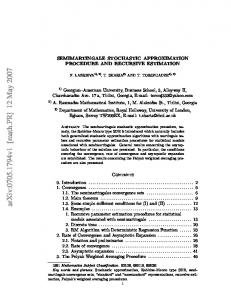
be used. For this study, we developed SGROUP, an implementation of MGROUP using MH stochastic approximation methods. Instead of CGROUP, we used BGROUP as the basis of our comparison with SGROUP. Sinharay and von Davier (2005) had analyzed these data and found their extended form of the BGROUP program gave more accurate results than CGROUP. On a desktop computer running Linux with a 2.2 GHZ processor and 2 GB RAM, SGROUP used 304 iterations of the MH-algorithm and took approximately 31 minutes to converge when using a chain length of 200 MH draws. In contrast, the CGROUP program would take about 22 minutes to perform the convergence on the same machine. If the number of MH draws per iteration were increased, the time needed to converge would be increased proportionally. Figure 1 provides a comparison of estimated regression coefficients (i.e., estimates of components of Γ) as differences between CGROUP and BGROUP, and also for the differences between SGROUP and BGROUP, for each of the three subskills. For convenience of viewing, the range of the vertical scale in the plots in Figure 1 is the same. The differences between SGROUP and BGROUP are negligible and are as large as those between CGROUP and BGROUP. ˆ from BGROUP, CGROUP, and Table 1 compares the residual variance estimates Σ SGROUP. The differences of results produced by SGROUP and BGROUP are negligible and are mostly smaller than the small differences between the results produced by CGROUP and BGROUP. In addition, all three of the variance component estimates are slightly higher for CGROUP than for BGROUP, and all three correlations are slightly lower for CGROUP than for BGROUP. The estimated variances and covariances produced by SGROUP do not have such a systematic deviation from the BGROUP estimates. Figures 2 and 3 compare the differences between posterior means and standard deviations (SDs) of 10,000 randomly chosen examinees for CGROUP versus BGROUP estimates, and for SGROUP versus BGROUP estimates. Both figures have a plot for each subscale. For convenience, the range of the vertical scales in the plots are the same for CGROUP and SGROUP. 12
Figure 1. Comparison of regression coefficients from CGROUP, BGROUP, and SGROUP for the 2002 NAEP reading assessment at grade 8. The rightmost panels of Figure 2 show the differences roughly in the scale reported by NAEP. In operational NAEP, a weighted average of the scores on the three subscales (with weights 0.35, 0.45, and 0.20 for literacy, information, and performance, respectively) is reported. NAEP uses a complicated linking procedure involving data for grades 4, 8, and 12—this usually converts the composite score to a scale with mean of approximately 300 and an SD of approximately 35. For the 2002 NAEP reading assessment at grade 8, the 13
Table 1 Residual Variances, Covariances, and Correlations for the 2002 NAEP Reading Assessment at Grade 8 BGROUP Lit.
CGROUP–BGROUP
SGROUP–BGROUP
Inf.
Per.
Lit.
Inf.
Per.
Lit.
Literary
.517 .363
.339
.010
.004
.004
.004 -.002
.007
Information
.765 .435
.339
-.006
.009
.005
-.007 -.001
.002
Performance
.733 .800
.413
-.007
-.006
.010
.011
Inf.
.004
Per.
.002
Note. Residual variances are shown on main diagonals, covariances on upper off-diagonals, and correlations on lower off-diagonals.
reported mean of the composite was 264 and the SD of the composite was 35. We do not use the rigorous NAEP linking procedure here, but instead use a simpler alternative that involves computing the weighted average of the posterior means on the three subscales for each examinee, using the weights 0.35, 0.45, and 0.20, as used in NAEP. Then we apply a linear transformation of the resulting weighted average to convert it to a scale with a mean of 264 and an SD of 35. For the most part, results produced by SGROUP are close to those produced by BGROUP and closer than those produced by CGROUP. CGROUP has a tendency to overestimate high posterior means and underestimate low posterior means (the extent of underestimation being more severe, especially for a few examinees). CGROUP slightly overestimates the extreme posterior SDs, a phenomenon that was also observed by Thomas (1993) and von Davier and Sinharay (2007). The SGROUP does not have any of these limitations. Table 2 shows the subgroup means and SDs (in parentheses) from BGROUP and the difference in these values from SGROUP and BGROUP—there seems to be little difference between the results.
14
Figure 2. Comparison of the posterior means from CGROUP, BGROUP, and SGROUP for the 2002 NAEP reading assessment at grade 8. Math Grade 4 NAEP 2000 The 2000 math NAEP assessment in grade 4 has five subscales, namely, (a) number and operations, (b) measurement, (c) geometry, (d) data analysis, and (e) algebra. The sample consists of approximately 13,900 students. The number of items across all subscales and booklets was 173, and 387 predictor variables were included in the latent regression model. On a desktop computer running Linux with a 2.2 GHZ processor with 2 GB RAM, 15
Figure 3. Comparison of posterior standard deviations from CGROUP, BGROUP, and SGROUP for the 2002 NAEP reading assessment at grade 8. the program implementing SGROUP used 421 iterations of the MH-algorithm and took approximately 1.5 hours to converge. In contrast, it would take the same machine 2 hours to converge CGROUP. These values refer to the MH-algorithm with chain length of 200. Longer chains will result in longer run times. The SGROUP program allows one to vary the chain length and to increase it programatically after initial iterations with chain lengths as little as 100 in the early cycles, and up to 2,000 in the final cycles. Increasing the chain 16
Table 2 Comparison of Subgroup Estimates From BGROUP and SGROUP for the 2002 NAEP Reading Assessment at Grade 8 BGROUP Subgroup Overall
Literary Information
SGROUP–BGROUP Task
Literary
Information
Task
0.027
0.022
0.022
-0.001
0.000
0.000
(0.984)
(0.949)
(0.970)
(0.003)
(-0.001)
(0.001)
-0.116
-0.078
-0.133
-0.001
0.000
0.000
(0.983)
(0.962)
(0.967)
(0.002)
(-0.001)
(0.001)
0.170
0.123
0.178
0.000
0.000
0.000
(0.965)
(0.925)
(0.947)
(0.002)
(-0.001)
(0.002)
0.286
0.267
0.315
-0.001
0.000
0.001
(0.897)
(0.852)
(0.849)
(0.002)
(-0.001)
(0.002)
-0.497
-0.447
-0.516
-0.002
-0.001
-0.001
(0.935)
(0.897)
(0.903)
(0.004)
(0.000)
(0.001)
-0.408
-0.434
-0.516
-0.002
-0.000
-0.000
(0.982)
(0.981)
(0.982)
(0.003)
(-0.001)
(0.002)
0.137
0.200
0.124
0.000
0.001
-0.001
American
(0.959)
(0.944)
(0.940)
(0.003)
(-0.002)
(0.001)
American
-0.330
-0.299
-0.250
0.000
-0.001
-0.001
Indian
(0.946)
(0.922)
(0.953)
(0.002)
(-0.001)
(-0.003)
Male
Female
White
Black
Hispanic
Asian
length will increase estimation time and the accuracy of the estimates. Note that BGROUP is not applicable to this example, since the number of subscales in the mathematics example does not allow the evaluation of a fixed-grid numerical integration over five dimensions in limited time. Trials of BGROUP with four dimensions on a comparable personal computer took more than a week to achieve convergence. The results obtained indicate that both programs fill in numeric boundaries for the 17
residual correlation between the five subscales, which are known to be highly correlated, as all five math scales measure closely related quantitative skills in different subdomains of mathematics as taught in school. Therefore, the results have to be interpreted with some care. However, parameter estimates obtained by CGROUP and SGROUP are very similar; the correlations between regression coefficients obtained with CGROUP and SGROUP range between 0.9997 and 0.9914. Table 3 presents correlations between these estimates, and means and standard deviation of the estimates obtained by CGROUP and SGROUP. Table 3 Comparison of Means and Standard Deviations From CGROUP and SGROUP for the 2002 NAEP Reading Assessment at Grade 8 Scale correlation
1
2
3
4
5
0.99970 0.99909
0.99142
0.99844
0.99779
0.00069 -0.00055 0.00021
-0.00090
Mean CGROUP
-0.00059
Mean SGROUP
-0.00060 0.00066
SD CGROUP
0.02143
0.02274
SD SGROUP
0.02128 0.02242
-0.00053
0.00012 -0.00088
0.02199 0.02425
0.02385
0.02181
0.02325
0.02379
A scatterplot depicting the agreement between SGROUP and CGROUP with respect to the regression parameters obtained is presented in Figure 4. In this plot, only two of the five subscales are compared: Scale 1, with the highest correlation between CGROUP and SGROUP, and Scale 3, with the relatively lowest correlation of 0.991. As the direct comparison in the top row and the difference plots in the bottom row indicate, the relationship between the estimates obtained by CGROUP and SGROUP is closely matched by the identity line (X = Y). However, since the high correlations between subscales prevented both algorithms from converging without setting numerical bounds to residual correlations, further in-depth analyses of similarities and differences between the two approaches will not be carried out here. We note that in spite of the limits set on 18
Figure 4. Comparison of regression coefficients obtained for the NAEP math 2000 grade 4 data using the operational CGROUP and the stochastic approximation estimation method (SAEM) implemented in SGROUP. Note. Due to very high correlations for all subscales, only a subset of two subscales representing the range of results is presented. correlations, both algorithms provided very similar estimates for the regression coeffficients in this five-dimensional case.
19
6
Conclusions
This paper describes how a stochastic approximation method can be used in estimating latent regression models used in large-scale educational surveys such as NAEP. The examples presented in this paper compare the stochastic approximation approach to the operational numerical methodologies used in NAEP and other large-scale educational survey assessments. The results indicate that stochastic approximation can be used to avoid some of the technical assumptions underlying current operational methods. Among these are the assumptions used in the Laplace approximation in the operational CGROUP approach. Moreover, stochastic approximation methods rely on the draws from the posterior distribution of the statistic of interest. This allows one to generate imputations (plausible values) without the assumption of posterior normality. This is an advantage of the stochastic approximation methods, which may play out favorably in cases where, for example, due to reduced dimensionality of the background model or due to a limited number of items in the measurement model, the normality assumption used in the current operation approach may not be appropriate. The approach implemented in SGROUP enables one to draw plausible values without relying on a restrictive assumption about the form of the posterior distribution. Note, however, the convergence behavior of stochastic methods needs close monitoring. For this purpose, there is need for further investigations aimed at optimizing the choice of the annealing process in order to minimize the number of iterations needed while at the same time ensuring that the process obtains estimates that maximize the objective function.
20
References Adams, R. J., Wilson, M., & Wu, M. (1997). Multilevel item response models: An approach to errors in variables regression. Journal of Educational and Behavioral Statistics, 22(1), 47–76. Cai, L. (2007). Exploratory full information item factor analysis by a Metropolis-Hastings Robbins-Monro algorithm. Manuscript submitted for publication. Delyon, B., Lavielle, M., & Moulines, E. (1999). Convergence of a stochastic approximation version of the EM algorithm. The Annals of Statistics, 27(1), 94–128. Dempster, A., Laird, N., & Rubin, R. (1977). Maximum likelihood from incomplete data via the EM algorithm, Journal of the Royal Statistical Society: Series B, 39(1), 1–38. Gelman, A., Carlin, J. B., Stern, Hal, S., & Rubin, D. B. (1995). Bayesian data analysis. New York: Chapman and Hall. Gu, M. G., & Kong, F. H. (1998) A stochastic approximation algorithm with Markov chain Monte-Carlo method for incomplete data estimation problems. Proceedings of the National Academy of Sciences, USA, 95, 7270–7274. Gu, M. G., & Zhu, H. T. (2001) Maximum likelihood estimation for spatial models by Markov chain Monte Carlo stochastic approximation. Journal of the Royal Statistical Society: Series B, 63(2), 339–355. Hastings, W. K. (1970). Monte Carlo sampling methods using Markov chains and their applications. Biometrika, 57(1), 97–109. Kuhn, E., & Lavielle, M. (2004) Coupling a stochastic approximation version of EM with an MCMC procedure. European Series in Applied and Industrial Mathematics, Probability and Statistics, 8,115–131. Lord, F. M. & Novick, M. R. (1968). Statistical theories of mental test scores. Reading MA: Addison-Wesley. Metropolis, N., Rosenbluth, A. W., Rosenbluth, M. N., Teller, A. H., & Teller, E. (1953). Equations of state calculations by fast computing machines. Journal of Chemical Physics, 21(6), 1087–1092. Mislevy, R. J. (1984). Estimating latent distributions. Psychometrika, 49, 359–381. 21
Mislevy, R. J., Beaton, A. E., Kaplan, B., & Sheehan, K. M. (1992). Estimating population characteristics from sparse matrix samples of item responses. Journal of Educational Measurement, 29(2), 133–161. National Center for Education Statistics. (2002). NAEP reading assessment for grade 8 [data file]. Available from the NAEP Data Explorer Web site, http://nces.ed.gov/nationsreportcard/naepdata/ Robbins, H., & Monro, S. (1951) A stochastic approximation method. Annuals of Mathematical Statistics, 22, 400–407. Sinharay, S., & von Davier, M. (2005). Extension of the NAEP BGROUP program to higher dimensions (ETS Research Rep. No. RR-05-27). Princeton, NJ: ETS. Thomas, N. (1993). Asymptotic corrections for multivariate posterior moments with factored likelihood functions. Journal of Computational and Graphical Statistics, 2(3), 309–322. Thomas, N. (2002). The role of secondary covariates when estimating latent trait population distributions. Psychometrika, 67(1), 33–48. von Davier, M. (2003). Comparing conditional and marginal direct estimation of subgroup distributions (ETS Research Rep. No. RR-03-02). Princeton, NJ: ETS. von Davier, M., & Sinharay, S. (2007). An importance sampling EM algorithm for latent regression models. Journal of Educational and Behavioral Statistics, 32(3), 233–251. von Davier, M., Sinharay, S., Oranje, A., & Beaton, A. (2006). Statistical procedures used in the National Assessment of Educational Progress (NAEP): Recent developments and future directions. In C. R. Rao & S. Sinharay (Eds.), Handbook of statistics: Vol. 26. Psychometrics. Amsterdam: Elsevier.
22