STOCHASTIC APPROXIMATIONS OF PRESENT VALUE FUNCTIONS ´ HELENE COSSETTE
MICHEL DENUIT
´ Ecole d’Actuariat Universit´e Laval Sainte-Foy, Qu´ebec, Canada, G1K 7P4
Institut de Statistique Universit´e Catholique de Louvain Voie du Roman Pays, 20 B-1348 Louvain-la-Neuve, Belgium
[email protected]
[email protected]
JAN DHAENE Departement Toegepaste Economische Wetenschappen Faculteit Economische and Toegepaste Economische Wetenschappen Katholieke Universiteit Leuven Minderbroedersstraat, 5 B-3000 Leuven, Belgium
[email protected]
´ TIENNE MARCEAU E ´ Ecole d’Actuariat Universit´e Laval Sainte-Foy, Qu´ebec, Canada, G1K 7P4
[email protected]
November 20, 2000
Abstract The aim of this paper is to apply the method proposed by Denuit, Genest and Marceau (1999) for deriving stochastic upper and lower bounds on the present value of a sequence of cash flows, where the discounting is performed under a given stochastic return process. The convex approximation provided by Goovaerts, Dhaene and De Schepper (2000) and Goovaerts and Dhaene (1999) is then compared to these stochastic bounds. On the basis of several numerical examples, it will be seen that the convex approximation seems reasonable.
Key words and phrases: Dependence, Stochastic Dominance, Stochastic Annuities
R´ esum´ e. Le but de cet article est d’appliquer la m´ethode propos´ee par Denuit, Genest et Marceau (1999) afin d’obtenir des bornes sup´erieures ou inf´erieures au sens de la dominance stochastique sur la valeur actuelle d’une s´erie de flux financiers lorsque le taux d’int´erˆet ob´eit a` un processus stochastique donn´e. L’approximation au sens de l’ordre convexe propos´ee par Goovaerts, Dhaene et De Schepper (2000) et Goovaerts et Dhaene (1999) est ensuite compar´ee aux bornes ´evoqu´ees plus haut. Sur base de plusieurs exemples num´eriques, l’approximation convexe semble raisonnable. Mots-cl´ e: d´ependance, dominance stochastique, annuit´es stochastiques
1
Introduction
Let Vt be the present value at time 0 of an amount of αt paid at time t. The stochastic discounted value at time 0 of payments of amount αt made at times t = 1, 2, · · · , n is then given by Zn = V 1 + V 2 + · · · + V n .
(1.1)
Consider for instance an insurance company facing payments of amount αt at times t = 1, 2, · · · , n; the present value of these n deterministic payments is given by (1.1). The Vi ’s involved in (1.1) are obviously correlated, so that the convenient independence assumption for the summands in Zn is not realistic. As a consequence, an exact expression for the cumulative distribution function of Zn requires the knowledge of the joint distribution of the random vector (V1 , V2 , · · · , Vn ), which is in general not available. Goovaerts, Dhaene and De Schepper (2000) recently proposed to circumvent en dominating this problem by approximating Zn by means of a random variable Z the original Zn in the convex sense. If we denote by F1 , F2 , · · · , Fn the respective distribution functions of V1 , V2 , . . . , Vn involved in (1.1), Zen is given by en = F1−1 (U ) + F2−1 (U ) + · · · + Fn−1 (U ), Z
where U is a unit uniform random variable and the Fi−1 ’s are the quantile functions associated to the Fi ’s. We obviously have that EZn = E Zen and it can be shown that the inequalities en − d, 0} E max{Zn − d, 0} ≤ E max{Z
(1.2)
hold for any d ≥ 0 (that is, Zn is smaller than Zen in the convex order). en precedes Zn in the convex sense, the approximation Z en is considered Since Z as less favorable by all the risk-averse decision-makers, and the method is thus conen enjoys an explicit servative. Moreover, the cumulative distribution function of Z expression and is particularly easy to handle. On the basis of numerical illustrations performed in a situation where the exact cumulative distribution function of Zn can be obtained, Goovaerts et al. (1999) showed that the cumulative distribution functions of Zn and Zen seem to be rather close. The problem of estimating the distribution of Zn has been studied, among others, by Beekman and Fuelling (1991), De Schepper and Goovaerts (1992), Dufresne (1990), Frees (1990), Parker (1994c,1997), De Schepper, Teunen, Goovaerts (1994) and Vanneste, Goovaerts and Labie (1994). This paper aims to carry on with Goovaerts et al.’s (1999) approach by providing lower and upper bounds on Zn in the stochastic dominance sense, using the method proposed in Denuit, Genest and Marceau (1999). This approach also provides upper and lower bounds on the quantiles of Zn . In risk management, these quantiles correspond to the Value at Risk at different probability levels. Such bounds cannot be obtained with the aid of the convex approximation Zen . Indeed, we see from (1.2) that the stop-loss premium of Zen is an upper bound of the stop-loss premium of Zn ; more generally, Eφ(Zen ) is an 1
upper bound for Eφ(Zn ) for any convex function φ. However, there is in general no en ≤ z] (since indicator functions are not convex). relation between P [Zn ≤ z] and P [Z Another purpose of this work is to provide several numerical illustrations which enhance the practical interest of our approach. In these illustrations, we will examine the position of the cumulative distribution function corresponding to the convex en in the admissible region delimitated by the stochastic bounds on approximation Z en can Zn . As a byproduct of our results, the error in the approximation of Zn by Z be evaluated (in other words, we get an upper bound for the Kolmogorov distance en ). between Zn and Z
2
Stochastic bounds on Zn
In this section, we recall how to build two functions Fmin and Fmax such that the inequalities Fmin (t) ≤ P [Zn ≤ t] ≤ Fmax (t) for all t ≥ 0,
(2.1)
en ≤ t] ≤ Fmax (t) for all t ≥ 0. Fmin (t) ≤ P [Z
(2.2)
hold, as well as
To this end, we use the following result due to Denuit et al. (1999, Proposition 2). Let F1 , F2 , · · · , Fn be the respective cumulative distribution functions of V1 , V2 , . . . , Vn . Then, the cumulative distribution function FZn of Zn = V1 +V2 +. . .+Vn is constrained by (2.1) with ( n ) X Fmin (t) = sup max P [Vi < vi ] − (n − 1), 0 , (v1 ,v2 ,... ,vn )∈Σ(t)
i=1
and Fmax (t) =
inf
(v1 ,v2 ,... ,vn )∈Σ(t)
where
min
( n X i=1
)
Fi (vi ), 1 ,
Σ(t) = {(v1 , v2 , . . . , vn ) ∈ IRn |v1 + v2 + . . . + vn = t}, t ∈ IR. Note that Fmax is a bona fide cumulative distribution function, whereas Fmin is the leftcontinuous version of some cumulative distribution function. The bounds in (2.1) and (2.2) are the best-possible bounds on Zn and Zen in the sense of stochastic dominance when we know the distribution functions F1 , F2 , . . . , Fn , but no assumption is made on the dependence structure between the Vi ’s. Equivalently, these bounds hold for all sums (1.1) with given cumulative distribution functions for V1 , V2 , . . . , Vn . Closed form expressions for the bounds (2.1) can in general not be obtained for distributions of the Vi ’s and one must resort to numerical evaluation. For more details, see Denuit et al. (1999). 2
Now, assume we have at our disposal some partial knowledge of the dependence existing between the Vi ’s, namely that there exists a multivariate cumulative distribution function G satisfying G(v1 , v2 , · · · , vn ) ≤ P [V1 ≤ v1 , V2 ≤ v2 , · · · , Vn ≤ vn ] for all v1 , v2 , . . . , vn ∈ IR, (2.3) and a joint decumulative distribution function H such that P [V1 > v1 , V2 > v2 , · · · , Vn > vn ] ≥ H(v1 , v2 , · · · , vn ) for all v1 , v2 , · · · , vn ∈ IR. (2.4) From Denuit et al. (1999, Proposition 5), the inequalities sup (x1 ,x2 ,··· ,xn )∈Σ(t)
G(x1 , x2 , · · · , xn ) ≤ FZn (t) ≤ 1 −
sup (x1 ,x2 ,··· ,xn )∈Σ(t)
H(x1 , x2 , · · · , xn ), (2.5)
hold for all t ∈ IR. The bounds in (2.5) are obviously more accurate than those in (2.1). In the literature, several notions of positive dependence have been introduced in order to express the fact that large values of one of the components of a random vector tend to be associated with large values of the others. In our context, one intuitively feels that in most situations the Vi ’s mainly “move together” (i.e. a large value of Vi is usually followed by a large value of Vi+1 ). For the numerical illustrations in this paper, we will assume that (2.3) and (2.4) are satisfied with G(v1 , v2 , · · · , vn ) = and H(v1 , v2 , · · · , vn ) =
n Y
n Y i=1
Fi (vi )
i=1
(1 − Fi (vi )).
In such a case, the Vi ’s are said to be Positively Orthant Dependent (POD, in short). POD comes thus down to assume that the probability that all the Vi ’s assume “small” values (i.e. Vi ≤ vi , i = 1, 2, . . . , n) is larger than the corresponding probability under the assumption that the Vi ’s are mutually independent. The interpretation for H is similar by substituting “large” for “small”. For more details, see, e.g., Szekli (1995, pp. 144-145).
3 3.1
Applications Stochastic annuities
Let δs be the force of interest at time s and let Yt denote the force of interest accumulation function at time t, i.e. Z t Yt = δs ds. s=0
3
The random present value at time 0 of a payment of 1 monetary unit at time t is given by exp(−Yt ), t ≥ 0. As noticed by Parker (1994b), there are mainly two possible approaches to model the interest randomness, namely the modeling of Yt and the modeling of δs . In the first approach, we could let Yt be the sum of a deterministic drift of slope δ and a perturbation modeled by a Wiener process, i.e. Yt = δt + σWt , t ∈ IR+ ,
(3.1)
where σ is a non-negative constant and {Wt , t ∈ IR+ } is a standardized Brownian motion. In such a case, Vt is log-normally distributed with parameters −δt and σ 2 t. This corresponds to the approach adopted by Goovaerts et al. (1999) who considered a discounted cash flow Zn of the form Zn =
n X i=1
exp(−δi − Xi ),
where the Xi ’s are assumed to be normally distributed with mean 0 and variance iσ 2 , and δ is the expected force of interest. The convex upper bound Zen on Zn obtained by Goovaerts et al. (1999) is Zen =
n X i=1
o n √ exp −δi − σ iΦ−1 (U ) ,
(3.2)
where Φ is the cumulative distribution function of a standard normal distribution and U is a random variable uniformly distributed on the unit interval [0, 1]. The survival function of Zen then follows from en > x] = 1 − F (x) = Φ(νx ), P [Z Zn
with νx the root of the equation n X i=1
αi exp(−δi −
√
iσνx ) = x.
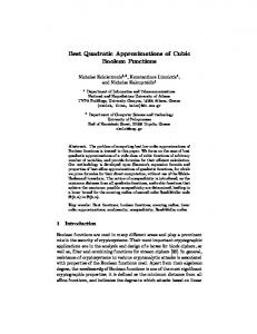
Let us now investigate the accuracy of the bounds (2.1) and (2.5) on the distribution function of Zn in the model (3.1). In Figure 1, one sees the functions Fmin and Fmax involved in (2.1). with in between the approximation FZn of the unknown FZn for n = 10, δ = 0.08 and σ = 0.02. Figure 3 is the analog for n = 20. Comparing the cumulative distribution function of the convex approximation (3.2) with the stochastic bounds (2.1), we see from Figures 1 and 3 that (3.2) lies in the very middle of the admissible region bordered by Fmin and Fmax . This indicates that (3.2) could be reasonable. In Figures 2 and 4, we further assume that the Vi ’s are POD and we computed the improved bounds furnished in (2.1). Only the lower bound got improved. As it is observed in Example 3 of Denuit et al. (1999), both upper and lower bounds on the distribution of a sum of random variables got improved when the 4
1.0 0.8 0.6 0.0
0.2
0.4
upper bd on Fa lower bd on Fa convex upper bd
4
6
8
10
Figure 1: Graph of the bounds (2.1) and cumulative distribution function of Z˜10 for (3.1) with δ = 0.08 and σ = 0.02. supports of the random variables are of the form [ai , bi ] with −∞ < ai < bi < +∞. If bi is equal to +∞ as in Example 1 of Denuit et al. (1999), only the lower bound will be improved with the assumption of POD. In our examples, the random variables are lognormally distributed with supports corresponding to [0, +∞). If, as in Goovaerts and Dhaene (1999), δt is defined by a CIR model, then Yt will be strictly positive, Vt = exp(−Yt ) will take values between 0 and 1, and therefore upper and lower bounds on the distribution of Zt will have been improved. A second approach to model interest randomness is to model δs . For instance, the force of interest can be defined by the differential equation dδt = −α(δt − δ)dt + σdWt ,
(3.3)
with non-negative constants α and σ, and with initial value δ0 = δ ≥ 0; {δt , t ≥ 0} is thus an Ornstein-Uhlenbeck process. The force of interest accumulation function {Yt , t ≥ 0} is therefore a Gaussian process with mean function t 7→ µt = δt + (δ0 − δ)
1 − exp(−αt) , α
and autocovariance (s, t) 7→ Cov[Ys , Yt ] ≡ ω(s, t), where ω(s, t) =
σ2 σ2 min(s, t) + {−2 + 2 exp(−αs) + 2 exp(−αt) α2 2α3 − exp(−α(t − s)) − exp(−α(t + s))} ; 5
1.0 0.8 0.6 0.0
0.2
0.4
upper bd on Fa lower bd on Fa convex upper bd lower bd on Fa with POD
4
6
8
10
0.6
0.8
1.0
Figure 2: Graph of the bounds (2.5) and cumulative distribution function of Z˜10 for (3.1) with δ = 0.08 and σ = 0.02.
0.0
0.2
0.4
upper bd on Fa lower bd on Fa convex upper bd
5
10
15
20
Figure 3: Graphs of the bounds (2.1) and cumulative distribution function of Z˜20 for (3.1) with δ = 0.08 and σ = 0.02. 6
1.0 0.8 0.6 0.0
0.2
0.4
upper bd on Fa lower bd on Fa convex upper bd lower bd on Fa with POD
5
10
15
20
Figure 4: Graphs of the bounds (2.5) and cumulative distribution function of Z˜20 for (3.1) with δ = 0.08 and σ = 0.02. see e.g. Parker (1994a, Section 6). Then, Zn =
n X
exp(−Yi ),
i=1
where Yi is a Normal random variable with mean µi and variance ω(i, i). In such a case, the convex upper bound Z˜n follows from Goovaerts et al. (1999): en = Z
n X i=1
n o p exp −µi − ω(i, i)Φ−1 (U ) ,
where U is a random variable uniformly distributed on the unit interval [0, 1]. In Figure 5, you can see the bounds on the cumulative distribution function of Z10 in the model (3.3) with δ = 0.06, δ0 = 0.08, α = 0.3 and σ = 0.01, together with the cumulative distribution function of Z˜10 . Figure 7 is the analog for n = 20. The comments inspired from Figures 1 and 3 still apply. In Figures 6 and 8, we assumed that the Vi ’s were POD. Again, the improvement with POD is moderate.
3.2
Life insurance
Consider a temporary life annuity issued to an individual aged x with curtate-futurelifetime K and denote P [k < K ≤ k + 1] = k| qx and P [K > n] = n px . We assume 7
1.0 0.8 0.6 0.0
0.2
0.4
upper bd on Fa lower bd on Fa convex upper bd
5
10
15
20
0.6
0.8
1.0
Figure 5: Graphs of the bounds (2.1) and cumulative distribution function of Z˜10 for (3.3) with δ = 0.06, δ0 = 0.08, α = 0.3 and σ = 0.01.
0.0
0.2
0.4
upper bd on Fa lower bd on Fa convex upper bd lower bd on Fa with POD
4
6
8
10
Figure 6: Graphs of the bounds (2.5) and cumulative distribution function of Z˜10 for (3.3) with δ = 0.06, δ0 = 0.08, α = 0.3 and σ = 0.01. 8
1.0 0.8 0.6 0.0
0.2
0.4
upper bd on Fa lower bd on Fa convex upper bd
5
10
15
20
0.6
0.8
1.0
Figure 7: Graphs of the bounds (2.1) and cumulative distribution function of Z˜20 for (3.3) with δ = 0.06, δ0 = 0.08, α = 0.3 and σ = 0.01.
0.0
0.2
0.4
upper bd on Fa lower bd on Fa convex upper bd lower bd on Fa with POD
5
10
15
20
Figure 8: Graphs of the bounds (2.5) and cumulative distribution function of Z˜20 for (3.3) with δ = 0.06, δ0 = 0.08, α = 0.3 and σ = 0.01. 9
that K is independent of the random discount factors V1 , V2 , V3 , . . . . The net single premium relating to this contract is given by ax;n| = E[a◦x;n| ], with a◦x;n|
0 if K = 0, ZK if K = 1, . . . , n − 1, = Zn if K ≥ n,
where Z is defined as in (1.1). By conditioning on K, the net single premium relating to such a contract is n−1 X ax;n| = E[Zk ]k| qx + E[Zn ]n px . k=1
The cumulative distribution function of a◦x;n| is also obtained by conditioning on K: P [a◦x;n| ≤ y] = qx +
n−1 X k=1
P [Zk ≤ y]k| qx + P [Zn ≤ y]n px .
No explicit expression exists for P [a◦x;n| ≤ y], but we use the approach developed above allows us to find stochastic dominance bounds on a◦x;n| . In Figure 9, we depicted the graph of the bounds on P [a◦x;n| ≤ y] for an individual aged 45 in the model (3.1) with δ = 0.08 and σ = 0.02. Figure 10 is the analog in model (3.3) with δ = 0.06, δ0 = 0.08, α = 0.3 and σ = 0.01. For these numerical illustrations, we used the standard mortality table (Makeham model) given in Bowers et al. (1996). The bounds in Figures 9 and 10 give a good idea of the danger inherent to the stochastic interest rate combined with the stochastic mortality. Let us mention that the convex approximation of Goovaerts et al. (1999) also applies in this situation.
Acknowledgements Partial funding in support of this work was provided by the Natural Sciences and Engineering Research Council of Canada and the “Chaire en Assurance l’IndustrielleAlliance”.
References [1] Beekman, J.A., and C.P. Fuelling (1991). Extra randomness in certain annuity models. Insurance: Mathematics & Economics 10, 275-287. [2] Bowers, N.L., Gerber, H.U., Hickman, J.C., Jones, O.A. and C.J. Nesbitt (1996). Actuarial Mathematics. Society of Actuaries, Itasca, Illinois. [3] Denuit, M., Genest, C. and E. Marceau (1999). Stochastic bounds on sums of dependent risks. Insurance: Mathematics & Economics 25, 85-104. 10
1.0 0.8 0.6 0.4 0.2
upper bd on Pr(B10