Defense Technical Information Center ... tain interference, cold clutter and possible targets (unsupervised training samples) are available for any type of.
UNCLASSIFIED
Defense Technical Information Center Compilation Part Notice ADP014047 TITLE: Stochastic-Constraints Method in Nonstationary Hot-Clutter Cancellation Part II: Unsupervised Training Applications DISTRIBUTION: Approved for public release, distribution unlimited Availability: Hard copy only.
This paper is part of the following report: TITLE: Military Application of Space-Time Adaptive Processing [Les applications militaires du traitement adaptatif espace-temps] To order the complete compilation report, use: ADA415645 The component part is provided here to allow users access to individually authored sections f proceedings, annals, symposia, etc. However, the component should be considered within
-he context of the overall compilation report and not as a stand-alone technical report. The following component part numbers comprise the compilation report: ADP014040 thru ADP014047
UNCLASSIFIED
8-I
Stochastic-Constraints Method in Nonstationary Hot-Clutter Cancellation
-
Part II: Unsupervised Training Applications
Prof. Yuri I. Abramovich 1,2 1 Surveillance Systems Division, Defence Science and Technology Organisation (DSTO) PO Box 1500, Edinburgh S.A. 5111, Australia 2 Cooperative Research Centre for Sensor Signal and Information Processing (CSSIP) SPRI Building, Technology Park-Adelaide, Mawson Lakes S.A. 5095, Australia yuri@cssip .edu. au
Abstract We consider the use of "stochastically constrained" spatial and spatio-temporal adaptive processing in multimode nonstationary interference ("hot clutter") mitigation for scenarios that do not allow access to a group of range cells that are free from the backscattered sea/terrain signal ("cold clutter"). Since supervised training methods for interference covariance matrix estimation using the cold-clutter-free ranges are inappropriate in this case, we introduce and analyze adaptive routines which can operate on range cells containing a mixture of hot and cold clutter and possible targets (unsupervised training samples). Theoretical and simulation results are complemented by surface-wave over-the-horizon data processing, recently collected during experimental trials in northern Australia.
1.
Introduction
In this lecture, we continue our study into the adaptive spatial and spatio-temporal mitigation of nonstationary interference in the field of high frequency (HF) over-the-horizon radar (OTHR). The preceding lecture discussed the fundamental ideas behind the new "stochastic-constraints" approach, which has been proposed to achieve effective hot-clutter suppression whilst maintaining distortionless output cold-clutter post-processing stationarity. The introduced operational implementation is based on the availability of range cells specifically free of cold clutter, a situation that is quite typical of pulse-waveform (PW) OTHR. Meanwhile, even within the PW OTHR architecture, attempts to increase the radar duty cycle (ie. the transmitted energy) usually lead to multifrequency operation with a transmission pause for each given frequency, limited to the operational range depth. For surface-wave (SW) OTHR, such a multifrequency mode of operation leaves little room for (sea-) clutter-free ranges being available. For frequency-modulated continuous waveform (FMCW) OTHR, the accessibility of such range cells, containing interference/jamming and noise signals only, is also problematic. Traditionally, FMCW systems operatemwith a linear frequency-modulated (LFM) waveform and have receiving systems which employ a mixing of the received waveform with a time-delayed version of the transmitted waveform. This process is known as "deramping" and is followed by spectral analysis (weighted Fourier transform) within the comparatively narrow bandwidth of a low-pass filter at the output of the mixer. This bandwidth is usually adjusted to the operational range depth, so that the frequencies corresponding to the "skip zone" ranges are usually filtered out at this stage. Thus only "operational" range cells which contain interference, cold clutter and possible targets (unsupervised training samples) are available for any type of processing. Note that the "simple" solution of increasing the low-pass filter bandwidth has its limit because of the significant increase in range sidelobes, due to the frequency mismatch [1]. Unfortunately, these range sidelobes also smear the multimodal interference structure somewhat. Obviously the type of operational routines discussed in [2] based on access to cold-clutter-free ranges are not applicable to these types of OTHR. It is important to emphasize that most existing adaptive algorithms are unable to address the problem of effective interference and cold-clutter mitigation simultaneously. Indeed, the number of "sweeps" (or repetition periods, N) within the coherent processing interval (CPI, "dwell"), combined Paperprevented at the RTO SET Lecture Series on 'MilitaryApplication of Space-Time Adaptive Processing", held in Istanbul, Turkey, 16-17 September 2002; Wachtberg, Germany, 19-20 September 2002; Moscow, Russia, 23-24 September 2002, andpublishedin RTO-EN-027.
8-2
-
with the number of spatial receiving channels M, is typically too large to consider even slow-time-only STAP as a solution to this problem, since the problem has MN degrees of freedom, and we have M Al 32 to 64 and N = 128 to 256 for typical radar facilities. Not only is. this solution impractical for computational reasons, but the number of available range cells T wvithin the bandwidth of the above-mentioned low-pass filter is usually too small (T = 50 to 70) compared with the product MN to provide reliable convergence for the STAP filter to the efficiency given by the true (deterministic) covariance matrix as T --+ co. Moreover, this problem is aggravated if severe multimode ionospheric propagation [3, 4, 5, 6] gives rise to the so-called "hot-clutter" phenomenon, whereby a signal produced by a single interference source is seen as a multiplicity of interference signals at the receiving array. According to [4]: Ionospherically propagated signals may consist of several modes, nonstationary in bearing and highly correlated with each other. Furthermore, due to the signal being refracted from an inhomogeneous region, each mode can be considered to consist of a specular ray surrounded by a cone of diffracted rays. The resulting wavefront for each mode may therefore be far from planar. When the temporal support of such multimode is significant, fast-time STAP with Q consecutive range bins ("taps", Nyquist intervals) involved in adaptive processing is one way to enhance hot-clutter rejectability. In some situations this is the only way to reject multimode interference, especially if one of these modes affects the main beam of the receiving array [2]. Obviously if MN-variate slow-time STAP is considered to be impractical, this is much more the case for the "fully adaptive" MNQ-variate STAP described in [7, 8]. Thus from a practical viewpoint, we should consider a scheme whereby each "finger beam" is associated with an M-variate spatial-only adaptive process (SAP), or at most with an MQ-variate fast-time STAP for interference-only (hot-clutter) mitigation. The output signals of each beam should then be processed by some standard slow-time inter-sweep coherent processing technique. Most existing HF OTHR facilities adopt a weighted Fourier transform for the detection of moving targets in the Doppler frequency domain. Clearly these standard cold-clutter post-processing techniques can'only be effective if the properties of the (scalar) cold clutter signal at the output of the adaptive beamformer are not contaminated by beamformer fluctuations caused by adaptation. This consideration is of great importance, since spatial and spatio-temporal properties of the ionospherically propagated jamming signal (hot clutter) are highly nonstati onary over the CPI. One possible analytic model that involves variations of the ionospheric propagation medium during the CPI is introduced in [6], and further mentioned in [2]. While the interference mitigation efficiency of an adaptive filter that is constant over a CPI may be quite poor in such cases, we may achieve a substantial improvement only if the corresponding SAP or STAP system can track perturbations of the hot-clutter covariance matrix along the CPI. When perturbations of the antenna array pattern due to the tracking are unconstrained, we observe a significant degradation in the properties of the cold-clutter Doppler spectrum (peak-to-sidelobe ratio, "subclutter visibility") [2]. It has been demonstrated [9, 10, 11, 12, 2] that additional data-dependent ("stochastic") constraints could be imposed on adaptive interference rejection filters to maintain distortionless output cold-clutter processing stationarity. Here we introduce and analyze operational stochastically constrained (SC) SAP/STAP routines that implement the same fundamental principle, but for unsupervised training. The basic idea of the first introduced approach is straight-forward: we reject the cold clutter using a moving-target indicator (MTI), calculate the STAP weights from this data that will reject hot clutter but maintain cold-clutter stationarity, then apply these weights to the original data, enabling the cancellation of cold clutter using standard Doppler processing. When the MTI filter can be designed in a nonadaptive fashion, the implementation of this basic idea is quite simple, and appears to be already discussed in classified papers [13, 14, 15]. Therefore we concentrate on the efficiency analysis of this approach for typical HF OTHR scenarios. In the more general case when the cold-clutter spectral properties are unknown a priori,implementation of the basic idea is less trivial, and the hot-clutter-only rejection filter should be properly retrieved from the associated 3-D STAP.
8-3
2.
Operational Routine for Unsupervised Training
Our goal is now to construct a complementary operational routine which implements an approximated version of the generic solution for the unsupervised training scenario. We may formulate a similar approach, providing we can somehow obtain proper rejection of the hot-clutter component. Clearly we must be prepared to sacrifice some performance compared with supervised training, due to the absence of samples containing only hot clutter and noise. 2A1
Known (Local) Cold-Clutter Model
In [2], we demonstrated using real OTHR sea-clutter data that, despite the quite complicated natu~re of the seaclutter Doppler spectrum over the entire dwell, stabilization by stochastic constraints can be quite effective, even if we adopt a simplified local low-order AR model (ie. accurate only for a limited number of consecutive sweeps). In fact, it has long been known that a simplified one-stage MTI filter, for example, can effectively reject cold clutter even if this clutter is much more complicated than an ordinary Markov chain, when such a filter is truly optimal. According to the general philosophy discussed in Section I, our goal is to apply the "shortest" possible MTI filter to reject the backscattered cold-clutter first, in order to extract the hot-clutter samples that can be later used for hot-clutter covariance matrix sample averaging. Here it is crucial to involve the minimum possible number of repetition periods, due to the non'stationarity of the hot clutter, which increases the signal subspace dimension of the averaged covariance matrix/R'1. On the other hand, if the cold-clutter residues are significant, the hotclutter covariance matrix estimate will be significantly compromised. Since the AR model for SC purposes also needs to be of minimum possible order (tK), it could be used directly to design the MTI filter providing that the parameters bj (j 1,..., n) and a2 are known a priorior estimated. Thus we assume that a (r.+ 1)-variate slow-time preprocessing filter
kt = z4t
bbjik-i,t
+
for
k = n+1,...,N
(1)
j=1
would lead to effective cold-clutter mitigation within the output snapshot ikt, ie.
-
eir irl kt
=
T
+ RoJi~
lbJO jj=O
with bo
1
2 R2
2 IMQ + '77,M
(2)
1, and
Ro
A;E[j]!kf-j "(3)
This gives rise to the following straight-forward operational routine.
Algorithm 1 Step I Given the observed M-variate snapshots zkt (k = 1,..., N; t = 1,..., T), form the "stacked" MQ-variate samples ikt (k = 1,..., N; t = 1,..., T-Q+1). Step 2 Preprocess the samples ikt by the (r.+ 1)-variate slow-time preprocessing filter with impulse response [1, bl,..., bJ] to get the cold-clutter-free training samples i using (1).
8-4
Step 3 Compute the sample estimate of the hot-clutter-plus-noise averaged covariance matrix T-Q+1
Rik
- T-Q+1 k
T-Q+1
Zt=1
i.['
for
k=,K+l,...,N.
(4)
tk
Step 4 Construct the initial (k = ,z+ 1) STAP filter R+) 2 ~vav 4 0))[All(o) q = Bav~~~~~~~~
-1
/"I
A,
)
Note that this filter is stochastically unconstrained and so is range-invariant (w
e =,+,t =
5 (5)
'-+).
Step 5 For the next adaptive filter i-,t+ 2 (now range-dependent and stochastically constrained), apply "sliding window" averaging to the preprocessed input data ,+2,t. T-Q+1
a1
T-Q+
R,+2
I
:
(6)
K+2,t 'rH
in order to ensure hot-clutter rejection over the repetition periods k = 2,..., K+2. Compute all subsequent STAP filters (k = K+2, ... , N) by
"4.--= (Rkvy- Azt [A-u•'/
where
z av
Rk
=
Az ]kv)-1 eq-,
(h
(7)
1 T-Q+( T-Q+1 Y ZktZkt
(8)
t=l
and the system of stochastic constraints is
where 2k
[ikl,t
I4k-2,t
j i k-..,t]
(10)
Note that the particular parameters used- in [9, 2] to simulate HF scattering from the sea K=2,
bo= 1,
b6 =-1.9359,
b2=0.998,
cr! =0.009675
(11)
means that all three covariance matrices ?73(j = 1, 2, 3) are almost equally weighted by Jbjl2, while the cold-clutter component inik'+l,t is rejected to the level of the weak temporally white noise. In Step 5, note that the n repetition periods k = 2,..., n+ 1 are common in the construction of R,+I and
R,c+ 2. The system of r
stochastic constraints corresponding to Wk
-j,t
k.lt
zik-j,t
for
j=
l,...,
.
(12)
may then be written as Z+l,t•ikt =
Zs+2,tikt for
k=2,
,,•+1
(13)
8-5
It is worth emphasizing that the hot-clutter covariance matrix estimates are computed using the preprocessed samples , while the stochastic constraints use the original snapshots •it. Thus the right-hand sides of these constraints consist of the cold-clutter samples mainly due to the properties of the estimate (6), while condition (3) ensures that the filter i'V+ 2 ,t properly processes the cold-clutter samples, since the hot clutter is to be rejected. Our final comment is a reminder that the matrix in the square brackets in (5) has dimension q x q, while that of (7) is (q+r.) x (q+ni), since all STAP filters but the first have nvadditional data-dependent linear constraints. A comparison of this algorithm with its counterpart for supervised training (the subject of the previous lecture), reveals that the only significant difference between these two techniques is how we obtain the coldclutter-free training samples to estimate the hot-clutter-plus-noise covariance matrix. For unsupervised training, we heavily rely on the ability of the iv-ord~er slow-time filter rejecting the cold-clutter signal practically to the level of white noise. In this regard, we stress that such rejectability validates the use of a low-order AR coldclutter model. On the other hand, suitability of a low-order AR model to real cold clutter over a very limited number of repetition periods (ie. locally) does not mean that the same model is appropriate for describing cold clutter over the entire CPI (ie. globally). Therefore the proposed preprocessing cannot be used as a moving target indicator (MTI) filter as such since, for low-speed targets, this processing is far from being globally optimal and leads to an unacceptably broad range of "blind" Doppler frequencies. It is thus essential that the proposed preprocessing is applied only to extract hot clutter which is uniformly distributed over the entire Doppler frequency band, while, for proper target detection,. we retain the output scalar cold-clutter signal as close as possible to its original form. It was demonstrated in [2], by processing of real skywave and surface-wave OTHR data, that the loworder AR model supports the stochastic-constraints approach by preserving the global structure of the output scalar cold-clutter signal, which is more complicated than suggested by the model. In Section V, we shall demonstrate that the low-order AR model also provides effective real cold-clutter rejection by the associated preprocessing filter. Nevertheless, none of the preprocessing schemes can entirely reject real cold clutter and so some cold-clutter residues are always present within the training sample il . This means that additional losses are expected compared with supervised training, especially if these residues are above the white noise level. Another source of loss stems from a reduction in the training sample size: for supervised training we separately estimate each !k using the set of hot-clutter training samples within each repetition period k, while, for unsupervised training, we use only one set of (T - Q + 1) ranges to estimate a single matrix which approximates the sum of all (nv+ 1) matrices ! 2.2
Known Order of the (Local) Cold-Clutter Model
In some applItcitions it is reasonable to admit that a preprocessing MTI-type filter can be defined based on some fairly standard a prioriassumptions. In the field of SW OTHR, for example, such a local model might be inferred, from an analytical description of the sea-echo Doppler spectra [16]. In general, though, our prior information is much more limited. To accommodate this, we specify only the AR model order r. prior to data processing, while the actual parameters values bj are unknown. Therefore, both the cold-clutter temporal properties, as well as the hot-clutter spatial (for SAP) or fast-time spatio-temporal (for STAP) properties, are to be estimated simultaneously using the unsupervised data ikt. It should be clear that this can be achieved only by incorporating slow-time to deal with the cold clutter. The main idea behind the algorithm that we propose is again straight-forward. For the properly chosen AR model of order nv, the appropriate MQ(rv+ 1)-variate 3-D STAP filter fik.t should then effectively reject both hot and cold clutter. On the other hand, since the hot-clutter signal is uncorrelated over adjacent sweeps, effective mitigation will occur only if each of the (r.+ 1) fast-time MQ-variate 2-D STAP subfilters effectively rejects hot clutter. Thus, using the first MQ components of the 3-D STAP filter, we may reject the hot-clutter component, while the cold-clutter contribution should remain unperturbed. Clearly we are decomposing the overall 3-D STAP filter, extracting the component responsible for hot-clutter mitigation only.
8-6
Let us introduce the MQ(n+ 1)-variate "doubly stacked" vector
[Zk-r..,4
Zkt
=(14) Z1k--l,t
Lkt In the absence of a target signal, we may write C{e
}
--
C{ktxkt} X
-{ZktZkt}
Y{kttkt} ±
°Y•TIMQ(K+1)
(15)
since the hot- and cold-clutter signals are mutually independent. Correspondingly,
ER{
k}
C{XktX'kt} + 0
1Q(.+1)
=[~](16)
since the hot clutter is uncorrelated over adjacent repetition periods. For a cold-clutter component described by the scalar multivariate model Ykt +
>jjj=1
(17)
k-jt =
we have
E Rk=
C{1Jzkt~zk~t}1=
+l®0 6
(18)
where 7Z-.+== Toep [ro,.., r.]
(19)
rj (j = 0,..., r) are the inter-period (scalar) correlation lags, and /ty is defined by the correlation property Ykt't'} = J(t- t) Rk,
C{
(20)
and by (2). In order to justify some of our assertions, let us temporarily simplify our problem. Suppose we ignore the nonstationarity of the hot clutter over the interval of (r.+1) adjacent repetition periods, and let us assume that the cold-clutter spatial covariance matrix is diagonal,11e. Jy = IMQ. (The angular distribution of cold clutter is always assumed to be sufficiently wide to exclude any possibility that pure SAP can solve the problem; further discussion appears in [2].) Thus the covariance matrix Ro is always well-conditioned, and so this second assumption does not change the essence of the problem. Under these two simplifying assumptions, we may present the overall MQ (r,+l)-variate covariance matrix
Rk in the form CZikt
R
-
It is known [ 17] that ifAA and uA (s
-
mQ = 1,+, 8)!Rkf +JR.+1®')
(21)
1,..., m) are respectively the eigenvalues and eigenvectors of some ra-
variate matrix A, while ýB and YB (t = 1,..., n) correspond to some n-variate matrix B, then the eigenvectors
uq (j = 1,..., rn) of the matrix C = Im. B + A®I,
(22)
are given by =
uja ®tu
for
s=l,...,m;t=1,...,n
(23)
8-7
and correspond to the eigenvalues of C equal to (,\A + B). By this property, the MQ(n+l)-variate vector w'k which minimizes the overall hot- and cold-clutter power -'H •Z Wk
I
Rw•, lk
subject to
'H
zi
wz
Wk -
1
(24)
is given by R=.+1
k
(25)
where ui (,) denotes the eigenvector corresponding to the minimum eigenvalue of the indicated matrix. We 2. cr2/+ also have that the total output power is o2u These considerations illustrate two important issues. Firstly, when the specified order n; is sufficient for effective cold-clutter mitigation by the corresponding r.-variate MTI-type filter, "augmented" MQ (tr+1)-variate STAP can simultaneously reject hot and cold clutter. The hot-clutter rejection can be achieved up to the spatial (or more generally, fast-time spatio-temporal) optimum processing limit, while the cold-clutter rejection can be achieved up to the temporal optimum processing limit, ie. the simultaneous rejection is uncompromising on its effect on the other component. Secondly, each of the (n + 1) blocks of this filter effectively mitigates the hot-clutter component, since R•kr has a block-diagonal structure. Indeed, each of the MQ-variate components of the vector • in (25) is proportional to the minimum eigenvector of /i=7 Now suppose that the total sample size (T-Q+-1)used for (loaded) sample averaging in the calculation of zZ
Rk. [2] is sufficiently large to essentially approach the efficiency of the true (deterministic) value for the STAP filter Z -1 = (o (26)
jZ
where ;(0(o) =--
T(Oo)
I0
10 1,
, then we expect the first MQ-variate section of this "augmented"
solution to provide effective fast-time STAP rejection of the hot clutter for the kth repetition period. It was demonstrated in [2] that the minimal samplevolume sufficient for 3dB average losses compared with the ideal solution (25) double the signal subspace dimension (ie. rank) of the noise-free covariancematrix. Since the covariance matrix rank is comparatively small, we may introduce the following operational routine.
Algorithm 2 Step 1 Given the observed M-variate snapshots zkt (k = 1,---, N; t = I..., T), form the "stacked" MQ-" variate samples ikt (k = 1,..., N; t = 1,.. ., T-Q + 1), and the "doubly stacked" MQ(K.+ 1)-variate samples ilt (k = + 1,..., N; t = 1,..., T- Q +1) using (14). Step 2 Compute the (loaded) sample covariance matrix estimates _z RZ
1
T-Q+1
= T-Q+ I
E
H Z-t Zkt + Ce lMQ(•+i)
(27)
t=1
for k
r'+ 1,..., 2i+ 1 and some small constant oa, then compute the averaged matrix =
1
j=0
(28)
8-8
Step 3 Let A.7 (00)
then define the initial (k = K+ 1) stochastically unconstrained
q[AT (00) 10 1... 1
and range-independent MQ(tc+ 1)-variate filter -1
/+ ava
1-
/_R,
: (q(o)F H
The first MQ elements of this vector form the first fast-time STAP filter av -1+'t
T = EMT
+1
e.
(29)
ie.
wU+lt
(30)
w here E M Q = [IM Q 1 ... 1O 1]T0. Step 4 For the next fast-time STAP filter
L,.+2,t
pute the MQ
by applying "sliding window" averaging:
+ 1)-variate filter
=+2,
(now range-dependent and stochastically constrained), com-
=
(31)
R2+l+ .
1
in order to ensure hot-clutter rejection over the repetition periods k = 2, ... " av(k=r.+ 2,.., Compute all subsequent operational fast-time STAP filters Wk t ki= W•
"tbkt
j)
=
where -
1-
=ik
Akt
K -z k+j,
l 7
~0°
N) by .,
a Wkt E1"Q
(32) (2
LAkt
A,
-:z
Aki =
eq+A
(33)
[-zT
LAkt IO1...Io
(34)
and the system of stochastic constraints is
A t =
[A,(0) 00-vH I
M(Im -
.
(35)
Wk-1 t -4(o)/
where Zk• is defined by (10). In Step 3, while the entire MQ (n+l)-variate filter wa+l,t would provide effective cancellation for both hot and cold clutter, we expect that constructing a fast-time STAP vector W1+,,t from its first MQ elements will deliver equally effective cancellation of the hot clutteronly, over the first (r+1) repetition periods. This will be true provided that the number of degrees of freedom in the vector exceeds the rank of the averaged hot-clutter covariance matrix R,+P,ie. MQ >> (.+1) [P(L+Q-1)]
(36)
or more precisely, taking into account the number of deterministic and stochastic constraints: MQ > (K+1) [P(L+Q-1)] + (q+n). In Step 4, for our standard example of r. = 2, once again the initial filter
(37) rejects hot clutter over
8-9
the repetition periods k
rejects over k
1, 2, 3, while the second filter wi
2, 3,4, thus ensuring that n
za, SZ
covariances R& are common for each successive average/A ensures the stationarity of the cold-clutter component is z avH
W 4V
and in general
Z
EMQZkt
avH
- W 4V
• vn.
wkt
Zkt =
avH
W3t
EMQikt
o._.vH _:(9 Zk._j,t = Wkt Zkj,t
.
-
The system of r. stochastic constraints which avH
W3 r
Zkt
for
k=2,...,n+1
(38) - -
-
for j
=
,...,.
(39)
Thus both sides of these constraints will consist mainly of cold clutter, since the hot-clutter component is rejected. As usual, the stochastic-constraints approach forms the kernel of this algorithm. The main difference with all previous routines is the method of separating hot and cold clutter: here we embed the fast-time STAP solution into the more general "augmented" 3-D STAP one to extract the desired solution as the component of the MQ (r.+ 1)-variate filter. It should be clear that the augmented STAP is only suitable for extracting the fast-time STAP solution, and cannot be used by itself as a final operational routine for target detection. As before, this is because the very small number of slow-time lags (n) involved in cold-clutter mitigation leads to a wide range of "blind" Doppler frequencies, where any targets would be rejected along with the cold clutter.
3.
Operational SC STAP Algorithm: Simulation and Real Data Processing
Naturally both of the proposed operational algorithms need to be verified. The most important question for Algorithm I is the relevance of the low-order AR cold-clutter model, and this shall now be addressed by real data processing, since there is no point filtering simulated cold clutter of a known AR model. The other important question on the convergence rate of the process to the true value as T --+ o for Algorithm 1 has been partly addressed in our previous papers on supervised training [9, 18, 2] with the established sample size T = 2(r+ 1)[P(L+Q-1)] necessary to guarantee average losses of 3dB compared with the optimal solution. Thus in order to justify the first operational routine we have to demonstrate that via a low-order AR model we can construct a preprocessing MTI-type filter that can efficiently reject cold clutter. -Firstly, we make use of the same real SW OTHR data as in [2], where the CPI is 100 seconds. The solid line in Fig. 1(a) shows the standard Doppler spectrum for one particular range cell; note that the subclutter visibility (the main-peak-tosidelobe ratio) is approximately 50dB in this case. Forward and backward averaging has been used to define the 3 x 3 (r = 2) inter-sweep temporal covariance matrix t,3. The preprocessing filter has been defined as W3-= (k3
e3
3-
3)
e3]
(40)
in order to keep unchanged the white-noise output power (since [1w311 = 1). The dotted line in Fig. 1(a) illustrates the Doppler spectrum of the residues after preprocessing. We see that the "noise floor" obtained by this pre-filtering is essentially the same as in the initial spectrum. Moreover, the eigenvalues of the sample matrix 7k3 A1 = 3.42, A2 = 0.0833, \ 3 = 0.0020 (41) suggest that the cold clutter could be rejected by about 27dB compared to the input level. This agrees with the subclutter visibility, taking into account the compression gain of N = 1000 repetition periods (L_30dB). Note that Fig. 1(a) also confirms our expectation of the very wide "blind" Doppler bandwidth which makes this type of processing inappropriate for target detection. Fig. 1(b) illustrates similar processing results of data obtained from DSTO's HF SWR facility located at Port Wakefield, South Australia. This radar employs a 16-element linear receiving array and operates over the frequency band 5 - 17M1z. The LFMCW waveform sweep rate and bandwidth are selectable over a wide
8-10
range; typically the waveform repetition frequency is around 4Hz and the bandwidth 50kHz. Since the repetition period is almost three times longer than in the previous data, the energetic components of the sea-clutter Doppler spectrum (solid line) obviously occupy a significantly wider range of relative Doppler frequencies. Consequently, the third-ordcr preprocessing filter (n = 2) shown by the dotted line is not extremely effective, rejecting the most prominent Bragg lines barely to the noise floor level. The "peak-to-noise" ratio at the output of this preprocessing filter (followed by a standard weighted FFT) is about 30dB, while the initial subclutter visibility is about 65dB. Nevertheless, if we increase the order of the AR model to n = 3, then the corresponding fourth-order preprocessing filter (dashed line) rejects all input energetic cold-clutter components far below the input white noise level. Thus for typical SW OTHR data, small-order AR models are proven to provide quite effective cold-clutter suppression, in turn enabling effective hot-clutter-only sample extraction. Verification of the second operational routine is not so simple, but the following two important questions may be addressed by simulation studies. Firstly, we need to demonstrate that for some standard hot- and cold+ clutter models, hot-clutter alone can be rejected by an MQ-variate component of the "augmented" MQ(± 1)-variate optimal solution. This optimal solution is constructed from the exact covariance matrix, and is interpreted as the limit solution, when the number of training samples tends to infinity. Secondly, we need to demonstrate that the convergence rate with respect to T is sufficiently high, since the number of range bins available in most HF OTHR applications is usually limited. The following simulations are based on the simple scenario of pure SAP with an M = 16 clement antenna array and a single fluctuating jamming source. The generalized Watterson model described in [6, 2] has been used to simulate the spatial and temporal (Doppler) fluctuations of the jammer. The spatial and temporal correlation coefficients have been chosen to reflect typical spatial fluctuations which make traditional mitigation techniques ineffective; in the notation of [2], these parameters are ("i = 0.90 and pit = 0.89 respectively, with 50dB HCNR and 0 i' = 59.1 degrees. The second-order AR model with N = 256 sweeps per dwell and the parameters of (11) have again been used to simulate HF scattering from the sea surface. Fig. 2(a) shows the Doppler spectrum for the cold clutter, uncorrupted by any jamming signal, at the output of the conventional beamformer (curve labeled "CBF Y"). We see that the subclutter visibility benchmark is approximately 80dB, which is an upper bound for most practical situations. Also illustrated is the Doppler spectrum of the coldclutter signal at the output of the standard (unconstrained) optimal SAP/STAP filter: iVST'AP =
-
(0o)
(42)
(note that here /?-r = R/"r and . (0o) = s(0o), since Q = 1) (the look direction is Oo = 0). Clearly the spatial nonstationarity of the jammer leads to a significant degradation in subclutter visibility (,-. -30dB), due to the fluctuations of the spatial (antenna array) weight vector. For this simulation, the instantaneous (per sweep) hotclutter-to-cold-clutter ratio (HCCCR) per antenna array element was chosen to be 0dB, so that the subelutter visibility for the conventional beamformer ("CBF Z") is also about 50dB. Therefore in this particular case, as far as the final subelutter visibility is concerned, conventional hot-clutter mitigation is as ineffective as no hot-clutter mitigation at all. Fig. 2(b) shows the results of our analysis into the limit efficiency of the algorithm described by Eqns. (32)(35), calculated by replacing the sample matrix Rk by the true covariance matrix Rk , ie. the sample volume is infinitely large. The curve labeled "long Z" presents the power of the total output signal for the "augmented" MQ(K+ 1)-variate STAP filter tb"; "long Y" shows the power of the cold-clutter component at the output of this filter; "long X" corresponds to the hot clutter power for the same filter, while "short X" illustrates the hot the truncated 16-element SAP filter .',I, simply formed from the first 16 elements clutter output power from vector Zat. of the 48-variate We see that in the given scenario, the hot-clutter component is rejected far below the level of the coldclutter residues at the output of the augmented STAP filter z a. Not surprisingly, the short filter - kt rejects the hot clutter slightly better than the augmented filter due to the independence of the hot clutter over adjacent
8-11
repetition periods. Thus the potential effectiveness of the proposed routine is extremely high, since the scalar output of the operational filter consists almost entirely of cold clutter only. The most important remaining question deals with finite sample size. In this regard, Fig. 2(c) differs from the previous figure only by the use of the finite sample size T = 41. For this reason, the "gap" between the hotand cold-clutter residues is smaller than in the previous case using deterministic covariance matrix calculations. Nevertheless, this gap is still large enough to guarantee that the hot-clutter component at the output of the filter wkt will be negligible. Correspondingly, the Doppler spectrum of the total signal at the output of the operational filter Z,, (curve labeled "Op SC STAP" in Fig. 2(d)) is practically indistinguishable from the cold-clutter-only component Doppler spectrum at the output of the conventional beamformer ("CBF Y"), and from the spectrum of the signal at the output of the SC STAP filter computed with the true covariance matrix ("Det SC STAP"). Thus the ability of the operational routine to suppress fluctuating jamming signals and to retain the initial subclutter visibility (very high in this example) is verified in this case. In order to explore the limitations of the proposed technique within the framework of the adopted model, we conducted similar simulations for input HCCCRs equal to I 0dB, 20dB and 30dB (Figs. 3, 4 and 5 respectively). We see that only in the (worst) last case does the hot-clutter output power approach the power of the cold-clutter residues at the output of the augmented adaptive filter zav. Meanwhile, subclutter visibility at the output of the operational filter wvt is degraded up to the level of about 70dB, compared with the initial value of about 80dB. It is worth mentioning that even for this worst case (HCCCR=30dB), the potential efficiency of hot-clutter mitigation is still extremely high. This means that with an appropriate sample volume, one can approach the initial subclutter visibility level Finally, we present some results of recent field trials to illustrate the efficiency of the supervised and unsupervised SC methods. The experimental facility involved has recently been developed near Darwin by the Australian Defence Science and Technology Organisation (DSTO), in collaboration with Telstra Applied Technologies (TAT) and the Cooperative Research Centre for Sensor Signal and Information Processing (CSSIP); the system was designed to function primarily as a SW OTHR, though it can operate in a variety of other data acquisition modes. The facility consists of two transmit sites, at Stingray Head (65km south-west of Darwin) and Lee Point (10km north-east of Darwin), together with a receive site at Gunn Point (30km north-east of Darwin) [19]. The receiving system is based on a 32-element uniform linear array, some 500m long, connected to a high dynamic range 32-channel HF receiver. The antenna element noise figures for the operational frequency range of 5-10MHz do not exceed 5dB, with a figure of near 1.5dB at the middle of the band. Such an antenna design permits a maximum possible external-to-internal noise ratio, and thus enables efficient external noise mitigation. Our results illustrate an example of low-power transmitter operation, where the last 30 or so range cells of the 80 available ranges have the sea-clutter signal deeply submerged into the environmental noise. Therefore we were able to use these last 30 ranges-for supervised training, and compare the efficiency of supervised and unfsupervised training SC techniques against the conventional beamformer (CBF) and standard SAP beamformer averaged over the entire dwell. For unsupervised training, we use the last 75 ranges, since the first five ranges are affected by the extremely strong direct-wave propagation. Algorithm I has been employed with the 30 range cells involved in cold-clutter AR parameter estimation for the MTI-filter design, averaging across all antenna array elements. Figs. 6-8 present the detailed range profiles for the target range cell 19 and 37, and the target-free range 12. The total noise power across the frequency bins 32 to 224 has been calculated to compare the signal-to-noise ratio improvement (SNRI) with respect to the CBF, bearing in mind that in the look direction (ideal planar wavefront), all beamformers are normalised to the same gain. Interestingly, this analysis demonstrates that unsupervised training (10-15dB SNRI) is slightly better than supervised training (8713dB SNRI) in this case. This could be explained by an improved interference averaging with most of the available ranges involved (75 out of 80). Practically, though, this improvement is not indicated by the actual SNRIs for the reference targets. This discrepancy between the expected and actual SNRIs is once again explained by the fact that the MTI residues that contain the target components have been used for interference covariance matrix estimation. Since perfect antenna calibration is
8-12
not attainable in practice, some degradation in SNRI is inevitable. This is a well-known phenomenon, and a straight-forward modification that excludes target-suspicious range cells from averaging provides one antidote. Nevertheless, both SC SAP options demonstrate the considerable improvement achievable in practice compared with CBF and averaged SAP in this environmental noise situation.
4.
Summary and Conclusions
We have extended the domain of practical application of the stochastic-constraints (SC) method to unsupervised training scenarios, typical of existing FMCW OTHR systems. Two operational routines have been proposed here. The first technique includes "slow-time" preprocessing of the input data by the MTI-type filter that can suppress the cold-clutter component far below the jamming signal level. We have demonstrated by real SW OTHR data processing that effective cold-clutter rejection can be achieved by involving avery modest number of repetition periods in preprocessing. In fact, the order of the preprocessing filter is equal to the order of the AR cold-clutter model, which in turn is equal to the number of stochastic constraints that secure the stationarity of the output cold-clutter signal. It is highly significant that low-order AR models have now been proven to be adequate only for the local description of the cold clutter, ie. over a very small number of consecutive repetition periods. Correspondingly, the preprocessing approach that we have introduced can only be used for the extraction of the hot-clutter signal, and is completely inappropriate for target detection due to the unacceptably broad "blind" Doppler frequency bandwidth. Within this first approach, the AR model, and consequently the preprocessing filter, are assumed to be known a priori(or estimated). The second, more general approach, relies only upon the chosen order of prepocessing filter sufficient for cold-clutter rejection, while the second-order moments for both hot and cold clutter are unknown. In this second method, the desired fast-time SAP/STAP hot-clutter rejection filter is defined as part of the "augmented" STAP filter which involves (n+1) consecutive repetition periods for additional cold-clutter mitigation. More precisely, the MQ-variate fast-time operational STAP filter (or M-variate SAP filter) ! is defined as the vector consisting of the first MQ (or M) elements of the augmented MQ(K+ 1)variate STAP filter (or the M(n+ 1)-variate STAP filter) Wki,. While at'v this augmented filter w t simultaneously provides both hot- and cold-clutter rejection, the short version Wkt was demonstrated to reject effectively only the hot-clutter component, far below the cold-clutter signal level. The proposed stochastic-constraints method ensures the stationarity of the scalar cold-clutter signal at the output of the operational filter Zwjt. Simulation results presented demonstrate that, for a typical scenario, the SC technique provides effective jammer mitigation, retaining the initial high level of subclutter visibility. These simulations involved a quite modest number of range resolution cells, typical of existing FMCW OTHR installations. The boundaries of usefulness of the SC method are explored in terms of subclutter visibility as a function of input hot- to coldclutter ratio. Most of the efficiency analysis results presented here are obtained by direct simulations, while a proper analytic study of the convergence properties of the SC approach remains to be done. Nevertheless, we have demonstrated by real SW OTHR data processing that unsupervised training scenarios typical of FMCW OTHR can be successfully treated in an operational mode using stochastic-constraints principles. Naturally the techniques introduced here could be useful for applications other than HF OTHR. The similarities between HF OTHR and airborne radar have already been discussed in [2].
References [1] D.E. Barrick, "FMCW radar signals and digital processing," NOAA Tech Report ERL 283-WPL26, 1973. [2] YI. Abramovich, N.K. Spencer, S.J. Anderson, and A.Y Gorokhov, "Stochastic-constraints method in nonstationary hot-clutter cancellation - Part I: Fundamentals and supervised training applications," IEEE Trans. Aero. Elect. Sys., vol. 34 (4), pp. 1271-1292, 1998.
8-13
[3] E.M. Warrington and C.A. Jackson, "Some observations of the directions of arrival of an ionospherically reflected HF radio signal on a very high latitude path," in Proc. Conf HFRadio Systems and Techniques, lEE Conf. Publ. No. 411, 1997, pp. 65-69. [4] M. Zatman and H. Strangeways, "The effect of the covariance matrix of ionospherically propagated signals on the choice of direction finding algorithm," in Proc. Conf.HF Radio Systems and Techniques, IEE Conf. Publ. No. 392, 1994, pp. 267-272. [5] C.M. Keller, "HF noise environment models," Radio Science, vol. 26 (4), pp. 981-995, 1991. [6] Y.I. Abramovich, C. Demeure, and A.Y. Gorokhov, "Experimental verification of a generalized multivarilte propagation model for ionospheric HF signals," in Proc.EUSIPCO-96,Trieste, 1996, vol. 3, pp. 1853-1856. [7] R. Fante and l.A. Torres, "Cancellation of diffuse jammer multipath by an airborne adaptive radar," IEEE Trans. Aero. Elect. Sys., vol. 31 (2), pp. 805-820, 1995. [8] S. Kogan et al., "Joint TS1 mitigation and clutter nulling architectures," in Proc. 5th DARPA Adv. Sig. Proc.Hot Clutter Tech. InterchangeMeeting, Rome Laboratory, 1997. [9] Y.I. Abramovich, V.N. Mikhaylyukov, and I.P. Malyavin, "Stabilisation of the autoregressive characteristics of spatial clutters in the case of nonstationary spatial filtering," Soviet Journalof Communication Technology and Electronics, vol. 37 (2), pp. 10-19, 1992, English translation of Radioteknika i Elektronika. [10] Y.I. Abramovich, F.F. Yevstratov, and V.N. Mikhaylyukov, "Experimental investigation of efficiency of adaptive spatial unpremeditated noise compensation in HFF radars for remote sea surface diagnostics," Soviet Journalof Communication Technology and Electronics,vol. 38 (10), pp. 112-118, 1993, English translation of Radioteknika i Elektronika. [11] Y.I. Abramovich, A.Y. Gorokhov, V.N. Mikhaylyukov, and I.P. Malyavin. "Exterior noise adaptive rejection for OTH radar implementations," in Proc.ICASSP-94, Adelaide, 1994, vol. 6, pp. 105-107. [12] Y.I. Abramovich and A.Y. Gorokhov,"AAdaptive OTHR signal extraction under nonstationary ionospheric propagation conditions," in Proc.RADAR-94, Paris, 1994, pp. 420-425. [13] L.E. Brennan, "Cancellation of terrain scattered jamming in airborne radars," in Proc.ASAP-96, MIT Lincoln Laboratory, 1996. [14] T.H. Slocumb, J.R. Guerci, and P.M. Techau, "Hot and cold clutter mitigation using deterministic and adap5tive filters," in Proc. 5th DARPA Adv. Sig. Proc. Hot Clutter Tech. Interchange Meeting, Rome Laboratory, 1997. [15] D.J. Rabideau, "Advanced stap for TSI modulated clutter," in Proc.ASAP-98, MIT Lincoln Laboratory, 1998. [16] D.E. Barrick, "Remote sensing of sea state by radar," in Remote Sensing of the Troposphere, V.E. Derr, Ed. Government Printing Office, Washington DC, 1972, Chapter 12. [17] R.A. Horn and C.R. Johnson, MatrixAnalysis, Cambridge University Press, England, 1990. [18] Y.I. Abramovich, A.Y. Gorokhov, and N.K. Spencer, "Convergence analysis of stochastically-constrained sample matrix inversion algorithms," in Proc.ISCAS-96, Atlanta, USA, 1996, vol. 2, pp. 449-452. [19] "Innovative radar for export," AustralianDefence Science, vol. 6 (3), pp. 12, 1998.
8-14
120
100-
80
120
80-
20' 201 -256 -56
-19 --192
-
128 -128
6418 00 -64 -64 64 (z frequency reaieDoppler reaieDoppler frequency (z
1892
1915
(b) (b) o ets Fiue11os-lorcmaio2nto0eso
: elsrac-aeOH
aa
2456
8-15
~
00
U
0
0
U
i-
U
C
C)
z
0 I-7
L
00
0
0
%oo 0
0
0)
01
N
0
000
0a
7
EHP .....
UP
i1...._-
II
IM
S0 0
0
00
ooI
"........{..
*
cIM. M
0
IIC)
ON
00z
.. '-I..49...
0.
\0
Oip
.
. :..
0'.
C
tip
Figure 3: Same simulation as in Fig. 2 but for a hot-clutter-to-cold-clutter ratio (HCCCR) of I0dB.
0ý0
8-17
N>--
.
00
0
in
U
0
"a
7
..
.....
00.
-C-
00 inR
II
F-
00
at
0
0
I
-
0
NO0i
i
I
C'.l
0
0 0
0 0
0
I0
I
I
II
Oqw
7
00
ýO
Tc
.2.
00CD
0
0
\0
0t
00 7i
E'0
li
Fiue4
aesmlto
si
i.2btfra
oUlte-ocl-lte
ai
H
C
R
fM
8-18
0
00
-ý
C.
0D
I4
0
x
~0
=
-'
0L!L
ir-.
00
-L
z-
N> Mw
0e
X w
4C)
In
c)
zU
H~00
0.
Z
0
0 'n
00
0
I'D
0
-
-.
00 00
C~.
H4D
iuaina
I
I
I
0 11~
00
0
C )o
0
IT
up
aH
5:Sm Figure
0Z
nFg,2btfrahtcutrt-odcutrrtoP(C
8-19
range #12, dotted line: CBF, solid line: unsupervised SC SAP (SNRI 15dB) 407 20 I
I
0
I
II
I
6
-20 1
32
64
96
128
160
192
224
256
relative Doppler
range #12, dotted line: constant SAP (SNRI 4dB), solid line: supervised SC SAP (SNRI 1 dB) 40i 20
0
•.
II
-
I
I
I
.128 relative Doppler
160
192
-20 32
64
96
224
256
Figure 6: Comparison of "range cuts" for range cell 12. range #19, dotted line: CBF, solid line: unsupervised SC SAP (SNRI 13dB) 60,
I
40 20
S0 -20 -40 32
60
64
96
128 relative Doppler
160
192
i 224
256
range #19, dotted line: constant SAP (SNRI 3dB), solid line: supervised SC SAP (SNRI 8dB) ,,,,
S20
"40 -20-40 32
64
i 96
128 relative Doppler
160
192
Figure 7: Comparison of "range cuts" for range cell 19.
i 224
256
8-20
range #37, dotted line: CBF. solid line: unsupervised SC SAP (SNRI 10dB) 40,
-20 1
32
I
I
I
I
64
96
128 relative Doppler
I
I
I
160
192
224
256
range #37, dotted line: constant SAP (SNRI 2dB), solid line: supervised SC SAP (SNRI 8dB) 40, ".::
m20
-20 -
:' 32
64
96
128 relative Doppler
160
192
Figure 8: Comparison of "range cuts" for range cell 37.
224
256