Stochastic Dependency Parsing Based on A* Admissible Search

Sixth SIGHAN Workshop on Chinese Language Processing

Stochastic Dependency Parsing Based on A* Admissible Search Bor-shen Lin National Taiwan University of Science and Technology / No. 43, Keelung Road, Section 4, Taipei, Taiwan [email protected]

sky and Martin 2001). To parse sentences with constituency grammar, a set of grammar rules written in linguistics is indispensable, while a corpus of tree bank annotated manually is also necessary if stochastic parsing scheme is adopted. In addition, the many non-terminal or phrasal nodes make it sophisticated to further interpret or disambiguate the parse trees since deep linguistic knowledge is often required. All these factors make language understanding very difficult, labor-intensive and not easy to be ported to various tasks.

Abstract Dependency parsing has gained attention in natural language understanding because the representation of dependency tree is simple, compact and direct such that robust partial understanding and task portability can be achieved more easily. However, many dependency parsers make hard decisions with local information while selecting among the next parse states. As a consequence, though the obtained dependency trees are good in some sense, the N-best output is not guaranteed to be globally optimal in general.

昨天 打 好 的 報告 寄 給 老闆 把 with yesterday type well of report send to boss

In this paper, a stochastic dependency parsing scheme based on A* admissible search is formally presented. By well representing the parse state and appropriately designing the cost and heuristic functions, dependency parsing can be modeled as an A* search problem, and solved with a generic algorithm of state space search. When evaluated on the Chinese Tree Bank, this parser can obtain 85.99% dependency accuracy at 68.39% sentence accuracy, and 14.62% node ratio for dynamic heuristic. This parser can output N-best dependency trees, and integrate the semantic processing into the search process easily.

1

(Send to the boss the report typed well yesterday.) 寄 send 給 to

把 with 報告 report

老闆 boss

的 of 打 type 昨天 yesterday

好 well

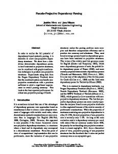
Figure 1. An example of dependency parsing with unlabeled dependency tree.

Introduction

Constituency grammar has long been the main way for describing the sentence structure of natural language for decades. The phrase structure of sentences can be analyzed by such parsing algorithms as Earley or CYK algorithms (Allen, 1995; Juraf45

Dependency grammar, on the other hand, describes the syntactic and semantic relationships among lexical terms directly with binary head-modifier links. Such representation is very simple, compact,

Sixth SIGHAN Workshop on Chinese Language Processing

direct, and therefore helpful for simplifying the process of language understanding and increasing task portability. Figure 1 shows an example of dependency parsing for the Chinese sentence “ 把昨 天打好的報告寄給老闆”(meaning “ send to the boss the report typed well yesterday” ). According to the binary head-modifier links, it is pretty easy to transform the dependency tree into the predicate “ send(to:boss,object:report(typed(yesterday,well))) ”for further interpretation or interaction, since the semantic gap between them is slight and the mappings are thus quite direct. Furthermore, robust partial understanding can be achieved easily when full parse is not obtainable, and measured precisely by simply counting the correct attachments on the dependency tree (Ohno et al., 2004). All these will not be so simple provided that conventional constituency grammar is used. In the dependency parsing paradigm, several deterministic, stochastic or machine-learning-based parsing algorithms have been proposed (Eisner, 1996; Covington 2001; Kudo and Matsumoto, 2002; Yamada and Matsumoto, 2003; Nivre 2003; Nivre and Scholz, 2004; Chen et al., 2005). Many of them make hard decisions with local information while selecting among next parse states. As a consequence, though the obtained dependency trees are good in some sense, the N-best output is not guaranteed to be globally optimal in general (Klein and Manning, 2003). On the other hand, A* search that guarantees optimality has been applied to many areas including AI. Klein and Manning (2003) proposed to use A* search in PCFG parsing. Dienes et al. depicted primarily the idea of applying A* search to dependency parsing, but there is not yet formal evaluation results and discussions based on the literatures we have (Dienes et al., 2003). In this paper, a stochastic dependency parsing scheme based on A* admissible search is formally presented. By well representing the parse state and appropriately designing the cost and heuristic functions, dependency parsing can be modeled as an A* search problem, and solved with a generic algorithm of state space search. This parser has been tested on the Chinese Tree Bank (Chen et al., 1999), and 85.99% dependency accuracy at 68.39% sentence accuracy can be obtained. Among three types of proposed admissible heuristics, dynamic heuristic can achieve the highest efficiency

46

with node ratio 14.62%. This parser can output Nbest dependency trees, and integrate the semantic processing into the search process easily.

2

Fundamentals of A* Search

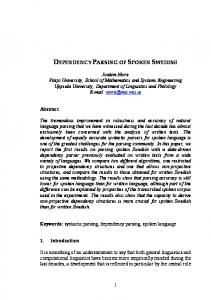
Search is an important issue in AI area, since the solutions of many problems could be automated if they could be modeled as search problems on state space (Russell and Norvig, 2003). A well known example is the traveling salesperson problem, as shown in the example of Figure 2. In this section basic constituents of A* search will be depicted. 2.1

State Representation

State representation is the first step for modeling the problem domain. It involves not only designing the data structure of search state but indicating the way a state can be uniquely identified. This is definitely not a trivial issue, and depends on the how the problem is defined. In Figure 2, for example, search state cannot be represented simply with the current city, because traveling salesperson problem requires every city has to be visited exactly once. The two nodes of city E on level 2 in Figure 2, with paths A-B-E and A-C-E respectively, are therefore regarded as different search states, and generate their successor states individually. The node E with the path A-C-E, for example, can generate successor B, but the one with the path A-B-E cannot due to reentry of city B. In other words, the search state here is the path, including all cities visited so far, instead of the current city. However, if the problem is changed as finding the shortest path from city A to city F, the two paths A-B-E and A-C-E can then be merged into a single node of city E with shorter path tracked. In such case, the search state will then be the current city instead of the path. A

Level 0 A

C B

Level 1

E

Level 2

D

C

B D

C E

B

E

F

F

Figure 2. An example of state space search for traveling salesperson problem from initial city A.

Sixth SIGHAN Workshop on Chinese Language Processing

In addition, for state representation three issues need to be further addressed.

open.add(initial); goal = search(); search() { while(true) { state = open.pop(); if(state.isGoal()) return state; successors = state.getSuccessors(); for(successor in successors) { if(!closed.contains(successor)) { closed.add(successor); open.add(successor); } } } }

‧ Initial state: what the initial state is. ‧ State transition: how successor states are generated from the current state. ‧ Goal state: to judge whether the goal state is achieved or not. In the above example in Figure 2, the initial state is the path containing city A only. The state transition is to visit next cities from the current city under the constraint of no reentry. The goal states are any paths that depart from city A and pass every city exactly once. 2.2

State Space Search

With the state well represented, two data structures are utilized to guide the search.

Figure 3. Generic algorithm for state space search. 2.3

Optimality and Efficiency

‧ An open list (a priority queue, denoted as open in Figure 3) used for tracking those states not yet spanned.

If the evaluation function f(n) satisfies

‧ A closed list (denoted as closed in Figure 3) used for tracking those states visited so far to avoid the reentry of the same states.

where g(n) is the real cost from the initial state to the current state n and h(n) is the heuristic estimate of the cost from the current state n to the goal state, such type of algorithm is called algorithm A. If further, the constraint of admissibility for h(n) holds, i.e.,

Then, a generic algorithm for state space search, with pseudo codes in object-oriented style shown in Figure 3, is performed to find the goal states. The initial state is first inserted into the queue, and an iterative search procedure (denoted as search() in Figure 3) is then called. For each iteration in the search procedure, the search state is popped from the queue and inspected one by one. If it is the goal state, the procedure terminates and returns the goal state. Otherwise the successors of the current state are generated, and inserted into the queue individually according to the priority provided not yet visited. The search procedure could be called multiple times if more than one goal states are desired. Note that the algorithm in Figure 3 is generic enough to be adapted for various search strategies, including depth first search, breadth first search, best first search, algorithm A, algorithm A* and so on, by simply providing different evaluation function f(n) of search state n for prioritizing the queue. For depth first search, for example, those states with the highest depth will have higher priority and be inserted at the front of the queue, while for breadth first search at the back. 47

f(n) = g(n) + h(n),

h(n) ≦ h*(n), where h*(n) is the true minimum cost from current state n to the goal state, then optimality can be guaranteed, or equivalently, the goal state obtained first will give minimum cost. Such type of algorithm is called algorithm A*. It can be proved that for algorithm A*, the closer the heuristic h(n) is to the true minimum cost, h*(n), the higher the search efficiency is.

3

A*-based Dependency Parser

In this section, how dependency parsing is modeled as an A* search problem will be depicted in detail. 3.1

Formulation

First, let W = {W1, W2, …,Wn} denote the word list (sentence) to be parsed, where Wi denotes the ith word in the list. And, each word Wi is expressed in the form,

Sixth SIGHAN Workshop on Chinese Language Processing

W = (w, t) (1) where w is the lexical term and t is the part-ofspeech tag. A dependency database can first be built by extracting the dependency links among words from a corpus of tree bank. Given the dependency database, a directed dependency graph G indicating valid links for the word list W can be constructed, as shown in the example of Figure 4. The direction of the link here indicates the direction of modification. Link W3  W2 in Figure 4, for example, means W3 can modify (or be attached to) W2. The dependency graph G will be used for directing the state transition during search. W1

W2

W7

W3

W6

W4 W5

Figure 4. Example dependency graph. 3.2

‧ Goal state: the set C is empty while all words in W are attached onto the dependency tree T. With the parse state represented well, the generic algorithm for state space search depicted in Section 2.2 can then be performed to find the N-best dependency trees. A partial search space based on the dependency graph G in Figure 4 is displayed in Figure 5, in which R denotes the root node of dependency tree. As shown in Figure 5, for each search state (denoted by the ovals enclosed with double-lines), only a link in form of Wj  R or Wj  Wi is actually tracked Through tracing the search tree back from the current state, all links can be obtained, and the overall dependency tree T can be constructed accordingly. For the search state W3  W2 in Figure 5, for example, the links W1 R, W2 W1 and W3  W2 are obtained through back tracing, which can then construct the dependency tree, W3  W2  W1  R, as can be seen on the left-hand side of Figure 5. This is similar to the case of traveling salesperson problem in Figure 2, in which only the current city is tracked for each state, but the path that identifies the search state uniquely can be obtained by back tracing.

Representation of Parse State

Since the goal of dependency parsing is to find the dependency tree, the search state can therefore be represented as the dependency tree constructed so far (denoted as T). Besides, a set containing those words not yet attached to the dependency tree (denoted as C, meaning “ to be consumed” ) can be generated dynamically by excluding those words on the dependency tree T from word list W. The three issues depicted in Section 2.1 are then addressed as follows.

T R W1

‧ Initial state: the dependency tree T is empty and the set C contains all words in list W.

W2

‧ State transition: a word is extracted from C and attached onto some node on the dependency tree T, and a successor state T’and C’is then generated. Whether an attachment is valid or not is determined according to the dependency graph G, under the constraints of uniqueness (any word has at most one head) and projectivity1 (Covington 2001, Nivre 2003).

W3

1

The projective constraint for new attachment is imposed by those attachments already on the dependency tree. Each attachment already on the tree forms a non-

48

W4,W5, W6,W7

Null

C W1  R

W2  R

W2  W1

W3 W2 W7 W3

W3 W1 R

W6 W1

R

W1 W2

…

W1 W3

W2 W6

Figure 5. A partial search space where some search states are associated with their dependency trees with dashed lines.

crossing region between its head and modifier to constrain new attachments for those words located within that region.

Sixth SIGHAN Workshop on Chinese Language Processing

3.3

Cost Function

For given word list W, the dependency tree T with the highest probability P(T) is desired, where P(T) = { P(WlR)}．{ P(Wj  Wi)}

(2)

The first term corresponds to those attachments on the root node of dependency tree (i.e. headless words), while the second term corresponds to the other attachments. In A* search, the optimal goal state obtained is guaranteed to give the minimal cost. So, if the cost function, g(n), is defined as the minus logarithm of P(T), g(n) ≡ -log (P(T))

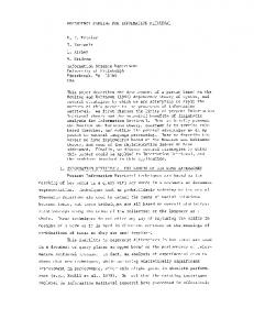
edly, the Baysian networks in Figure 6 appear too simple to model the real statistics precisely. In the link Wj Wi, for example, Wj might depend on not only its parent Wi but the children of Wi (Eisner, 1996). Also, the direction (sgn(i-j)) and the distance (|i-j|) of modification between Wi and Wj might be important (Ohno et al., 2004). All these factors could be taken into account by simply including the minus logarithms of the corresponding probabilities into the step cost. wl P(Wl | R)

= (–log(P(Wl R))) + (-log(P(Wj Wi)))

≡  step-cost

then the A* search algorithm that minimizes the cost g(n) will eventually maximizes the probability of the dependency tree, P(T). Here the minus logarithms of the probabilities in Equation (3), – log(P(Wl R)) and –log(P(WjWi)), can be regarded as the step cost for each attachment (or link) accumulated during search. Furthermore, since each word is expressed with a lexical term and a part-of-speech tag as shown in Equation (1), the probability for each link can be depicted as, P(Wl  R) = P(Wl | R) = P(tl|R)．P(wl|tl)

(4)

P(Wj  Wi) = P(Wj | Wi) = P(tj|ti)．P(wj|tj) (5) assuming the word list W is generated by the Baysian networks in Figure 6(a) and 6(b) respectively. Note that here the probability for a link P(Wj  Wi) involves not only the lexical terms wj and wi but also the part-of-speech tags tj and ti, and is denoted as link bigram. Such formulation can be generalized to high order link n-grams. Figure 6(c), for example, displays the Baysian network for the link Wk  Wj conditioned on Wj Wi, based on which the link trigram is defined as P(Wk  Wj | Wj Wi) = P(Wk | Wi, Wj) = P(tk | ti, tj)．P(wk | tk).

(6)

When comparing Figure 6(c) with Figure 6(d), the Baysian networks for link trigram P(Wk | Wi, Wj) and conventional linear trigram P(Wi+2 | Wi, Wi+1) respectively, it could be found that link n-gram is flexible for long-distance stochastic dependencies, though the two topologies look similar. Undoubt49

wi

tj

ti

P(Wj | Wi) tl

(3)

wj

R

(b)

(a) wk

wj

wi

wi+2

wi+1

wi

tk

tj

ti

ti+2

ti+1

ti

P(Wk | Wi , Wj) (c)

P(Wi+2|Wi , Wi+1) (d)

Figure 6. Baysian networks of (a) link unigram (b) link bigram (c) link trigram (d) linear trigram. 3.4

Heuristic Function

In A* search, the evaluation function f(n) consists of g(n), the real cost from the initial state to the current state n, and h(n), the cost estimated heuristically from the current state n to the goal state. Now for dependency parsing, g(n) defined in Equation (3) is the accumulated cost for those attachments on current dependency tree T, while h(n) is the predicted cost of the attachments for the words in C which have not yet been attached. Since h(n) ≦ h*(n) has to hold for admissibility, it is necessary to estimate h(n) conservatively enough so as not to exceed the true minimum cost h*(n). To achieve higher search efficiency, however, it is preferred to estimate h(n) more aggressively such that h(n) can be as close to h*(n) as possible. Therefore, in this paper, h(n) is estimated with the minimum of minus logarithms of link n-grams for each word in C, with different levels of constraints described below.

Sixth SIGHAN Workshop on Chinese Language Processing

‧ Global heuristic: the minimum is static, and can be calculated in advance before parsing any sentence by considering all link n-grams for each word. ‧ Local heuristic: the minimum is calculated according to the dependency graph G of current parsing sentence by considering all possible link n-grams with respect to G. ‧ Dynamic heuristic: the minimum is calculated dynamically according to current dependency tree T during parsing by considering only projective link n-grams with respect to G for current dependency tree T. By virtue of taking the minimum of minus logarithms of link n-grams, admissibility can be guaranteed for these heuristics. The latter with stricter constraints on finding the minimum can give more precise estimate of cost (with higher h(n)) than the former, and is thus expected to be more efficient, as will be discussed in the next section.

4

Experiments

The stochastic dependency parsing scheme proposed in this paper has been first tested on the Chinese Tree Bank 3.0 licensed by Academia Sinica, Taiwan, with six sets of data collected from different sources (Chen et al., 1999). Head-modifier links (with lexical term and part-of-speech tag) can be extracted from the tree bank since it is produced by a head-driven parser (Chen, 1996). In our experiments, One set, named as oral.check, containing 4156 sentences manually transcribed from dialogue database is used to train the dependency database, link statistics including conditional probabilities, link unigrams and bigrams as shown in Equation (4) and (5), and so on. Another set, named as ev.check, containing 1797 sentences in text books of elementary school is used to test the A*-based dependency parser. Note here the training corpus and testing corpus are of different domains, and each word in test sentences is transcribed into (w, t) format with lexical term w and associated part-of-speech tag t. 4.1

Coverage Rate

The number of occurrences and the coverage rate for the conditional probability P(wj|tj), link unigram P(tj) and link bigram P(tj|ti) respectively are shown in Table 1. As can be seen in this table, the 50

coverage rate for P(wj|tj) is as low as 50.8%, since the training and testing domains are quite different. The coverage rates for link unigram and bigram, however, can be up to 94.06% and 84.88% respectively. This implies that, the link probabilities can be estimated more appropriately and contribute more in finding the dependency trees. To handle the issue of data sparseness, in the following experiments a simple n-gram backoff mechanism is utilized for smoothing. No. of occurrences Training corpus Testing corpus Overlaps Coverage rate

P(wj|tj) 8137 2791 1418 50.80%

P(tj) 120 101 95 94.06%

P(tj|ti) 3383 1468 1246 84.88%

Table 1. Coverage rates for link statistics. 4.2

Parsing Accuracy

The experiment settings for dependency parsing are depicted as below. The first, denoted as BASE, is the baseline setting, while the others describe the search conditions applied to the baseline incrementally. The heuristic h(n) used here is the dynamic heuristic. ‧ BASE: baseline with the cost defined in Equation (3), (4) and (5). ‧ RP: root penalty for every root attachment Wl  R is included into the step cost. ‧ DIR: the statistics for the direction of modification, P(D|Wj  Wi)=P(D|ti, tj), is included into the step cost where D≡ sgn(j –i). ‧ NA: the statistics for the number of attachments (or valence), P(Ni|Wi)=P(Ni|ti), is included into the step cost and updated incrementally for every new attachment onto Wi. Ni is the current number of words attached to Wi. ‧ REJ: the obtained dependency trees are inspected one by one, and rejected if any of the conditions occurs: (a) the modifiers for conjunction word (e.g. “ 和” , meaning “ and” ) belong to different part-of-speech categories (in的”(meancorrect meaning) (b) illegal use of “ ing “ of” ) as leaf node (incomplete meaning). The baseline setting with Equation (3), (4) and (5) is based on the Baysian networks depicted in Fig-

Sixth SIGHAN Workshop on Chinese Language Processing

ure 6(a) and 6(b). Finer statistics could be applied in the settings RP, DIR and NA. The setting RP, for example, can restrain the number of headless words. The setting DIR can take into account the cost due to the direction of modification, since it in fact matters2, but the link probability P(Wj  Wi) in Equation (5) cannot differentiate between the two directions. The distance of modification, |j-i|, might matter too, but is not considered here due to quite limited amount of training data. The setting NA can include the cost due to the number of attachments. Verbs, for example, often require more attachments, and may produce lower cost for higher number of attachments. Here for simplification, the statistics of P(Ni|ti) are gathered only for Ni = 0,1,2, and >=3, respectively. In addition to using finer statistics, it is also feasible to use semantic or lexical rules to reject the dependency trees with incorrect or incomplete meanings. In the setting REJ, two rules are utilized. One is, the conjunction word should have modifiers in the same part-of-speech category, while the other is, the word “ 的”must have at least one modifier.

BASE + RP Cross + DIR Domain + NA + REJ BASE + RP Within + DIR Domain + NA + REJ

No. of Accurate Sentences 867 1039 1102 1211 1229 1109 1314 1340 1476 1484

SA

DA

48.25% 57.82% 61.32% 67.39% 68.39% 61.71% 73.12% 74.57% 82.16% 82.58%

77.42% 80.74% 82.72% 85.21% 85.99% 85.93% 89.91% 90.66% 92.81% 93.20%

Table 2. Parsing accuracy for various settings. The parsing performance can be measured with sentence accuracy (SA) and dependency accuracy (DA). Table 2 shows the experimental results for the above settings. The results for within-domain test by using the set ev.check for both training and testing are also listed here for comparison. It can be found in this table that, the performance of cross-domain test is not so good for the baseline

setting, but can be persistently improved when finer statistics are applied. Rejection of incorrect or incomplete dependency trees is also helpful (REJ), though very few semantic or lexical constraints are utilized here. When the constraints of all settings are applied, 85.99% dependency accuracy can be obtained at 68.39% sentence accuracy. 4.3

N-best Output

Note that due to data sparseness and the limitation of simplified Baysian networks, some parsing errors are intrinsic and difficult to avoid. Figure 7 shows the parsing result for a clause “ 吃晚飯的時 候”(meaning “ at the time for eating dinner” ). The incorrect parsing result on the right-hand side (meaning “ to eat the time of dinner” ) is syntactically correct and inevitable in fact, since the link probabilities (P(tj) or P(tj|ti)) dominate over the conditional probabilities (P(wj|tj)), as illustrated in Section 4.1. Such problem could possibly be alleviated to some extent if deep semantic constraints (e.g. a transitive verb may require a subject and an object) or lexical constraints (e.g. some adjectives may modify only specific nouns) could be utilized for rejection while reprocessing the N-best output. time

時候 (Nad)

eat

吃 (VC31)

of

的 (DE)

time

時候 (Nad)

eat

吃 (VC31)

of

的 (DE)

dinner

晚飯 (Naa)

dinner

晚飯 (Naa) incorrect result

correct dependency tree

Figure 7. The parsing result for the clause “ 吃晚 飯的時候”(time for eating dinner). Table 3 shows the experimental results of N-best output for the setting REJ. In Table 3 it can be seen that higher sentence accuracy, 80.08%, for top-5 output can be achieved, which implies large space for improvement in N-best processing. Top 1

Top 2

Top 3

Top 4

Top 5

SA 68.39% 75.24% 78.02% 79.41% 80.08%

2

In the Chinese phrase “ 在(in)…前面(front)” , for example, “ 在”is the head while “ 前面”is the modifier, and “ 前面” always modifies “ 在”backwards.

Table 3. Sentence accuracy for N-best output. 51

Sixth SIGHAN Workshop on Chinese Language Processing

4.4

References

Search Efficiency

The search efficiency for each test sentence can be measured heuristically by the order of complexity, defined as C = lognN

(7)

where n is number of words in the test sentence and N is the total number of the search nodes for that sentence. Cave is then used to denote the average complexity over all test sentences. In addition, Nall is the total number of search nodes for all test sentences, and can produce the node ratio RN when normalized. The experimental results for different heuristics depicted in Section 3.4 are shown in Table 4. As can be observed in this table, much higher search efficiency can be obtained for more precise heuristic estimate, but with compatible top 1 sentence accuracy. For dynamic heuristic with real-time estimate of the cost according to the current dependency tree, the highest efficiency can be obtained at 2.38 average complexity and 14.62% node ratio, respectively. Heuristic None Global Local Dynamic

SA 68.84% 68.34% 68.50% 68.39%

Cave 2.91 2.82 2.39 2.38

Nall RN 4748268 100% 3417766 66.29% 841716 17.73% 694193 14.62%

Chen K. J. 1996. A Model for Robust Chinese Parser, Computational Linguistics and Chinese Language Processing, Vol. 1, no. 1, pp. 183-205. Chen K. J., et al. 1999. The CKIP Chinese Treebank: Guidelines for Annotation, ATALA Workshop – Treebanks, Paris, pp. 85-96. Chen Yuchang, Asahara Masayuki and Matsumoto Yuji. 2005. Machine Learning-based Dependency Analyzer for Chinese, ICCC-2005. Covington Michael A. 2001. A Fundamental Algorithm for Dependency Parsing, Proc. of the 39th Annual ACM Southeast Conference, pp. 95-102. Dienes Peter, Koller Alexander and Kuhlmann Macro. 2003. Statistical A* Dependency Parsing, Proc. Workshop on Prospects and Advances in the Syntax/Semantics Interface. Eisner Jason M. 1996. Three Probabilistic Models for Dependency Parsing: An Exploration, Proc. COLING, pp. 340-345. Jurafsky Daniel and Martin James H. 2001. Speech and Language Processing, Prentice Hall, NJ. Klein Dan and Manning Christopher D. 2003. A* Parsing: Fast Exact Viterbi Parse Selection, Proc. NAACL/HLT.

Table 4. Search efficiency for different heuristics.

5

Allen James, 1995. Natural Language Understanding, The Benjamin/Cummings Publishing Company.

Conclusions

We have presented a stochastic dependency parsing scheme based on A* admissible search, and verified its parsing accuracy and search efficiency on the Chinese Tree Bank 3.0. 85.99% dependency accuracy at 68.39% sentence accuracy can be obtained under cross-domain test. Among three types of admissible heuristics proposed, dynamic heuristic can achieve the highest efficiency with node ratio 14.62%. This parser can output N-best dependency trees, and reprocess them flexibly with more semantic constraints so as to achieve higher parsing accuracy. This parsing scheme is the basis for natural language understanding in our research project on dialogue systems for mission delegation tasks. We plan to perform comparative studies with other non-stochastic approaches, and evaluate our approach on the shared task of dependency parsing.

52

Klein Dan and Manning Christopher D. 2003. Fast Exact Inference with a Factored Model for Natural Language Parsing, Proc. Advances in Neural Information Processing Systems. Kudo Taku and Matsumoto Yuji. 2002. Japanese Dependency Analysis using Cascaded Chunking, Proc. CONLL. Nivre Joakim, 2003, An Efficient Algorithm for Projective Dependency Parsing, Proc. International Workshop on Parsing Technologies (IWPT). Nivre Joakim and Scholz Mario. 2004. Deterministic Dependency Parsing of English Text, Proc. COLING. Ohno Tomohiro, et al, 2004. Robust Dependency Parsing of Spontaneous Japanese Speech and Its Evaluation, Proc. ICSLP. Russell S. and Norvig P. 2003. Artificial Intelligence: A Modern Approach, Prentice Hall. Yamada Hiroyasu and Matsumoto Yuji. 2003. Statistical Dependency Analysis with Support Vector Machines, Proc. IWPT