Stochastic differential equation models of vortex ... - Semantic Scholar

PHYSICS OF FLUIDS 17, 065107 共2005兲

Stochastic differential equation models of vortex merging and reconnection N. K.-R. Kevlahana兲 Department of Mathematics & Statistics, McMaster University, Hamilton, Ontario L8S 4K1, Canada

共Received 13 October 2004; accepted 12 April 2005; published online 3 June 2005兲 We show that the stochastic differential equation 共SDE兲 model for the merger of two identical two-dimensional vortices proposed by Agullo and Verga 关“Exact two vortices solution of Navier– Stokes equation,” Phys. Rev. Lett. 78, 2361 共1997兲兴 is a special case of a more general class of SDE models for N interacting vortex filaments. These toy models include vorticity diffusion via a white noise forcing of the inviscid equations, and thus extend inviscid models to include core dynamics and topology change 共e.g., merger in two dimensions and vortex reconnection in three dimensions兲. We demonstrate that although the N = 2 two-dimensional model is qualitatively and quantitatively incorrect, it can be dramatically improved by accounting for self-advection. We then extend the two-dimensional SDE model to three dimensions using the semi-inviscid asymptotic approximation of Klein et al. 关“Simplified equations for the interactions of nearly parallel vortex filaments,” J. Fluid Mech. 288, 201 共1995兲兴 for nearly parallel vortices. This model is nonsingular and is shown to give qualitatively reasonable results until the approximation of nearly parallel vortices fails. We hope these simple toy models of vortex reconnection will eventually provide an alternative perspective on the essential physical processes involved in vortex merging and reconnection. © 2005 American Institute of Physics. 关DOI: 10.1063/1.1932310兴 I. INTRODUCTION

Vortex interactions are fundamental to moderate and high Reynolds number flows. The dynamics of jets, fluidstructure interaction, and mixing layers are all governed by large-scale coherent vortices. It is also believed that the dynamics of high Reynolds number turbulence is dominated by vortex interactions. In particular, most enstrophy dissipation is probably due to the vortex reconnection. Many turbulent flows are forced by vorticity production at the wall, and drag reduction techniques attempt to modify the wall vortices. Vortex-based methods are used to simulate fluid flow in both two and three dimensions.1 It is thus clearly important to understand and analyze all stages of vortex reconnection. Unfortunately, there is still no simple mathematical model for vortex reconnection. This is because viscous diffusion is necessary for full vortex reconnection, and viscosity renders slender vortex models, with their relatively simple Hamiltonian dynamics, inapplicable. Despite this, many semi-inviscid models have been developed that include a steady approximation for core dynamics.2–5 These models fail once the vortices approach within a core radius, which leads to the development of a singularity in curvature 共called a hairpin or kink兲. Various more or less ad hoc ways of dealing with reconnection have been proposed.6,7 These methods use a physically based algorithm to give the end result of the reconnection. Obviously, the intermediate stages of the reconnection are not resolved. Of course, vortex reconnection can be calculated accurately using full direct numerical simulation 共DNS兲 of the Navier–Stokes equations.8,9 However, DNS is computationally expensive and gives little insight into the fundamental a兲

Electronic mail: [email protected]

1070-6631/2005/17共6兲/065107/11/$22.50

physical mechanisms involved. In addition, DNS is limited to moderate Reynolds numbers since its space-time computational complexity scales like Re3 共unless an adaptive method is used兲. For these reasons a simple analytic or semianalytic model for interacting vorticity filaments is desirable. Agullo and Verga10 claimed to have produced an “exact two vortex solution of the Navier–Stokes equations,” i.e., an equation for the interaction of two identical two-dimensional vortices whose solution can be approximated asymptotically. They simply took the inviscid equation for two interacting point vortices and turned it into a stochastic differential equation 共SDE兲 by adding white noise forcing. The positions of the point vortices become random variables, and the vorticity distribution is given by the probability density function 共PDF兲 for the positions of the point vortices. Although the equations do produce a single merged vortex, as we show in Sec. II, the dynamics and vorticity distribution are both quantitatively and qualitatively incorrect. In fact, the solution involves a severe simplification of the nonlinear term of the vorticity equation: only pairwise interactions between the point vortices are included in each realization. In the complete vorticity equations the vorticity at each point is advected by the vorticity at all other points simultaneously. It is this approximation that distinguishes Agullo and Verga’s approach from numerical vortex methods, where many point vortices are included simultaneously in order to approximate a continuous vortex distribution.1 Despite its shortcomings, Agullo and Verga’s approach does suggest a general way of extending inviscid models to include diffusion, and hence topology change. We will explore this idea, and try to evaluate its usefulness, in the present paper. The SDE toy models considered in this paper are closely related to, but distinct from, the stochastic vortex method introduced by Chorin.11 Chorin proposed his vortex method

17, 065107-1

© 2005 American Institute of Physics

Downloaded 21 Jun 2005 to 130.113.105.8. Redistribution subject to AIP license or copyright, see http://pof.aip.org/pof/copyright.jsp

065107-2

Phys. Fluids 17, 065107 共2005兲

N. K.-R. Kevlahan

as a way of efficiently solving the two-dimensional Navier– Stokes equations at high Reynolds numbers. The continuous vorticity field is divided into N vortex blobs, i.e., ␻ = 兺Nj=1␻ j, with the corresponding stream function, N

␺共r兲 = 兺 ⌫ j␺0共r − r j兲,

共1兲

j=1

where the smoothed kernel ␺0共r兲 is given by

␺ 共r兲 = 0

冦

1 ln r, 2␲ 1 r, 2␲␴

r 艌 ␴, r ⬍ ␴.

冧

共2兲

Distant vortex blobs interact as point vortices and ␴ is a cutoff which regularizes the logarithmic singularity of the point vortex kernel. The motion of the vortex blobs is then calculated by a split-step particle method where the particles are first advected using the streamfunction 共1兲共excluding self-advection兲, and then perturbed by a stochastic white noise forcing 共which models diffusion兲. Chorin saw this method as especially useful for high Reynolds number flows because it is gridless and because the error in approximating the advection term due to the random walk is O共Re−1/2兲. Chorin applied this simple vortex blob method to flow past a circular cylinder, where the no-slip boundary condition is enforced by the creation of M vortices 共of the appropriate strength兲 along the cylinder boundary at each time step. M depends on the time step: as the time step decreases more vortices must be created. In two dimensions the SDE model discussed in this paper is closely related to Chorin’s model. There are, however, several important differences compared with Chorin’s and other more recent vortex methods.1,12–14 共1兲 We use point vortices instead of vortex blobs. 共2兲 We consider only the interaction of initially wellseparated physical vortices. 共3兲 Each physical vortex is represented by only one point vortex. In vortex methods a large number 共typically tens or hundreds of thousands兲 of discrete vortices are used simultaneously.13,15 共4兲 The actual vorticity field is given by the ensemble average 共or PDF兲 of many realizations. Perhaps the most important difference, however, is our ultimate goal. We are not interested in the accurate numerical approximation of the vorticity equations 共vortex methods1,12–14,16–19 are already highly accurate in both two and three dimensions兲, but rather in the construction of simple toy models of vortex interaction which allow topology change. These models are not rigorously justified, but are intended to capture the minimal physics needed to qualitatively describe vortex interaction. In fact, the twodimensional case is just the simplest of a class of such SDE toy models that extend semi-inviscid vortex filament equations to include vorticity diffusion by the addition of white noise forcing. This converts the inviscid partial differential equation into a stochastic differential equation, where the

vorticity field is given by the PDF of its solution. These toy models should eventually give a new insight into the essential physics of vortex merger and reconnection, and can even admit analytical solution in certain cases.10 The paper is organized as follows. In Sec. II A we review Agullo and Verga’s SDE model for the interaction of identical two-dimensional vortices, and compare its solution with a full DNS in Sec. II B. The main source of error is identified and a simple correction is proposed in Sec. II C. This corrected model is shown to be qualitatively accurate. Then in Sec. III we extend the SDE model to the case of N interacting nearly parallel vortices via a simple modification of asymptotic semi-inviscid model by Klein et al.2 for nearly parallel vortices. Agullo and Verga’s model is a special case of this new model when N = 2 and vortex curvature is neglected. Because it is not a straightforward asymptotic approximation of the incompressible Navier–Stokes equations, the qualitative accuracy of this stochastic toy model is assessed by comparing it with a pseudospectral DNS of the reconnection of antiparallel vortices 共i.e., the Crow instability兲. Finally, we make some concluding remarks and outline future research directions in Sec. IV.

II. TWO-DIMENSIONAL TWO VORTEX SDE MODEL A. Basic model

Agullo and Verga10 proposed the following simple model for the interaction of two identical point vortices:

␺1 − ␺2 ⳵ ␺1 = 2i + 冑2␯⬘b1 , 兩 ␺ 1 − ␺ 2兩 2 ⳵t

共3兲

␺1 − ␺2 ⳵ ␺2 = − 2i + 冑2␯⬘b2 , 兩 ␺ 1 − ␺ 2兩 2 ⳵t

共4兲

where ␺ j共t兲 = x j共t兲 + i y j共t兲 are the positions of the two vortices 共expressed as complex numbers兲 and b j共t兲 are independent white noises 共the derivative of a Wiener process兲. Time has been rescaled by 4␲ so viscosity is also rescaled, ␯⬘ = 4␲␯. Note that the first term on the right-hand side is simply the 共nonlinear兲 advection by the other point vortex, and the second term is a white noise forcing which represents diffusion. The vortex positions ␺1 and ␺2 are random variables. The vorticity field is given by the ensemble average of many realizations of ␺1共t兲 and ␺2共t兲共which is an estimate of their PDFs兲, and the center of rotation of the vortices is given by the expectations 具␺1共t兲典, 具␺2共t兲典. In each realization the initial condition is the same: a pair of identical point vortices with circulation ⌫ = 1. Before considering the solution of the basic model 关共3兲 and 共4兲兴, let us recall the full two-dimensional vorticity equation,

⳵␻ = − u · ⵱ ␻ + ␯⌬␻ . ⳵t

共5兲

Note that the vorticity is confined to the z direction, i.e., ␻ = 共0 , 0 , ␻兲. The velocity is a functional of the vorticity, given by the Biot–Savart law,


065107-3


Stochastic differential equation models

boundaries兲. Again, this probabilistic model is only valid when many fluid particles are considered simultaneously. In contrast, in Agullo and Verga’s model each vortex is represented by only a single point vortex in each realization. Although the SDE model involves a rather severe approximation of the Navier–Stokes equations it does have some attractive features.

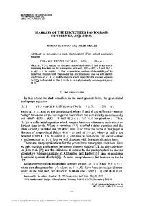
FIG. 1. Schematic illustration of the approximation to the nonlinear term in the basic SDE model. The shaded regions indicate the actual vorticity field and the black circles indicate the position of the point vortices in this particular realization. We are considering the velocity advecting vortex 1.

u共x,t兲 = −

1 2␲

冕

共x − y兲 ⫻ ␻共y,t兲dy, 兩x − y兩2

共6兲

where the integral is over the entire fluid. The interaction of two identical vortices corresponds to specifying an appropriate initial condition, e.g., with an initial separation r0,

␻共x,y;0兲 = ␦共− r0/2,0兲 + ␦共r0/2,0兲.

共7兲

This is also the initial condition used in the SDE model. Comparing 共6兲 with the SDE model, we see immediately that the SDE model involves a drastic simplification of the advection term. In fact, only the pairwise nonlinear interactions of point vortices are included in each realization. As we will see later, it is useful to divide the neglected part of the advection into two components: the advection of the point vortex due to self-advection 共i.e., due to the rest of the vortex兲 and the advection due to the vorticity of the rest of the other vortex 共i.e., due to the fact that the actual vorticity field is distributed and not concentrated at a single point兲. These neglected parts of the nonlinear advection are sketched in Fig. 1. The key approximation of the SDE model is thus a pointwise approximation to the advecting velocity field, where only one point 共which is itself a stochastic variable兲 is used in any given realization. Note that the effect of self-advection is entirely neglected in the SDE model. We will see that the neglect of self-advection is by far the largest source of error in this model. Interestingly, in the case of one vortex the SDE model is exact, since the nonlinear term is zero and the dynamics are purely diffusive. One can construct valid probabilistic approximations, or even representations, of the vorticity equations. For example, numerical vortex methods use a pointwise approximation of the vorticity field, but in this case the vorticity of a vortex is distributed over many point vortices 共e.g., tens of thousands兲. On the other hand, Busnello et al.20 have shown that one can construct an exact SDE representation of the vorticity of a three-dimensional viscous fluid on R3 共i.e., without solid

共1兲 Analytic solutions or approximations are possible in some cases 共e.g., Agullo and Verga10兲. 共2兲 Numerical solutions are efficient, even at large Reynolds numbers, because the method is gridless. In addition, the SDE model reduces the dimension of the vortex merger problem from two to zero 共i.e., from the continuous twodimensional vorticity equation to point vortex interactions兲. A similar SDE model 共see Sec. III兲 reduces the vortex reconnection problem from three dimensions to one dimension. 共3兲 Existing inviscid or semi-inviscid models can be extended easily to include topology change. This removes the finite time singularities associated with these models. 共4兲 The Hamiltonian structure of the original inviscid equations is retained. For these reasons it is interesting to evaluate the SDE model, and determine how it might be improved or extended. B. Comparison of the basic SDE model with a DNS

We now compare the basic SDE model solution with a full DNS. We use a high resolution adaptive wavelet direct numerical simulation 共WDNS兲 of the vorticity equation 共for details see Vasilyev and Kevlahan21兲. The WNDS uses an adaptive high-order explicit stiffly stable Krylov method in time.22 The key property of WDNS is that the computational grid adapts automatically to the solution at each time step, refining or coarsening locally as necessary. One can therefore think of the WDNS as a sort of constrained vortex method, where the adapted grid points correspond to vortices. Indeed, we use the fast multipole method23 approximation to the Biot–Savart law to find the velocity field given the vorticity at the adapted grid points. Thus, the number of points in the adapted grid gives an idea of the number of vortices required to fully represent the solution and its dynamics. The WDNS solution for the merger of two identical vortices with circulation ⌫ = 1 and initial separation r0 = 1 was computed at Re= ⌫ / ␯ = 1000 on a domain of 关−2.5, 2.5兴 ⫻ 关−2.5, 2.5兴 with a maximum resolution of 20482 grid points. The l2 norm tolerances for grid adaptation and time integration were set to 10−4. Note that the WDNS is dealiased: the actual grid used is twice as fine as the grid necessary to resolve the solution to the desired tolerance. The vorticity field at nine different times is shown in Fig. 2, while the associated adapted grid is shown in Fig. 3. Times are normalized by the initial rotation period of the pair of point vortices. Figure 4 shows that about 8000 grid points were used in the simulation, with a maximum of about 10 000 points at t = 1.37. This suggests that roughly 104 point vortices would be required simultaneously for a complete repre-


065107-4


N. K.-R. Kevlahan

FIG. 2. Vorticity field. Vortex merging at Re= 1000, full adaptive wavelet solution.

FIG. 4. Number of grid points in adaptive wavelet solution as a function of time.

sentation of the vorticity dynamics. Recall that only twopoint vortices are used in any given realization of the SDE model. The vortices are pushed together by the irrotational strain generated by the spiral vorticity filaments. This convective stage of merger is described in detail by Meunier24 and by Cerretelli and Williamson.25 The vortices are fully merged 共i.e., the vorticity field has a single maximum兲 after 1.5 pair rotation periods, and a single Gaussian vortex has formed after two rotations. The asymptotic long time state is therefore a single Gaussian vortex at the center of rotation of the initial conditions. The dynamics in the final stage are purely diffusive and therefore linear. We now solve the basic SDE model equations numerically, using the Euler–Maruyama method26 with a small time step of ⌬t = 10−4 to ensure accuracy. Note that since the drift coefficient 冑2␯⬘ is constant, the Euler–Maruyama method is equivalent to the Milstein method26 and has strong order 1. The vorticity field 共which is the ensemble average of 105

realizations兲 is shown in Fig. 5. A comparison of Figs. 2 and 5 reveals that the basic SDE model is both qualitatively and quantitatively incorrect. Although the long-time solution is a single Gaussian vortex in both cases, the intermediate dynamics and time scale for final merging are very different. In the basic SDE model the intermediate solution is a diffusing vortex ring, and the vortices have still not completely merged by t = 2.25. Indeed, merging is a diffusive process in the basic SDE model, whereas the actual merging process is advection dominated, with diffusion important only in the final stages.25 In the following section we propose a corrected model that gives a qualitatively accurate solution and identify the main source of error in the basic model.

FIG. 3. Adaptive wavelet grid for vortex merging at Re= 1000.

FIG. 5. Vorticity field. Vortex merging at Re= 1000, basic SDE model.

C. Corrected model

The error in the basic SDE model is due to the approximation of the nonlinear advection term by pairwise point vortex interactions. As mentioned above, this error may be divided into self-advection error 共neglected entirely兲 and


065107-5



TABLE I. Corrected SDE models. Case

Advecting velocities

Self-advection Other advection

U1 = u1 + V, U2 = u2 − V U 1 = u 2, U 2 = u 1

Both

U 1 = u 1 + u 2, U 2 = u 1 + u 2

other vortex interaction error 共the effect of the other vortex is approximated by concentrating all the vorticity at a single point兲. A pair of inviscid point vortices 共without white noise forcing兲 simply rotate around their center of rotation at a constant rate. We therefore propose to advect the point vortices in the SDE model by the velocity field of Gaussian vortices 共of the correct age兲 at the positions of the inviscid point vortices. It is easy to find an analytic expression for this velocity field. Because the velocity is an integral of the vorticity, we expect it to be relatively insensitive to the precise location and form of the vortices. Besides correcting the basic SDE model, this approach also allows us to separate the effects of self-advection and other vortex advection. The corrected equations are

⳵ ␺1 = iU1共␺1,t兲 + 冑2␯⬘b1 , ⳵t

共8兲

⳵ ␺2 = iU2共␺2,t兲 + 冑2␯⬘b2 , ⳵t

共9兲

where U1共z , t兲 and U2共z , t兲 are the 共complex兲 velocities advecting vortices 1 and 2, respectively.

Let u1 and u2 be the velocities of Gaussian vortices at the locations of inviscid point vortices with initial positions of vortices 1 and 2, respectively, and let V共␺1 , ␺2兲 = 2共␺1 − ␺2兲 / 兩␺1 − ␺2兩2 be the advecting velocity in the basic SDE model. In order to identify the main source of error in the basic SDE model we consider three different cases: selfadvection, other advection, and both, as summarized in Table I. Because the distance between the inviscid point vortices never decreases, we must eventually replace the two advecting Gaussian vortices by a single vortex at their center of rotation. Cerretelli and Williamson25 find that merging occurs when the vortex core size ␦ ⬇ 0.29r0. We use this time 共i.e., tc = 1.07兲 to switch to a single vortex. The single vortex must conserve the maximum vorticity and total circulation of the two vortices it replaces. Although this switch to a single vortex is rather ad hoc, it does give reasonable results. Note that for t 艌 tc all three models described in Table I are identical. The corrected SDE models are compared with the full WDNS solution in Fig. 6. Figures 6共c兲 and 6共d兲 show that the main source of error in the basic SDE model of Agullo and Verga is self-advection. If the effect of self-advection is approximated as described above, the solution of the SDE model is much more accurate. If the effect of the continuous vorticity of the other vortex is included as well, the SDE solution is qualitatively correct, and has approximately the right time scale. It is perhaps not surprising that selfadvection is the largest source of error: it is completely neglected in the basic SDE model. Although the goal of this paper is to develop and analyze the qualitative accuracy of simple SDE toy models for vortex

FIG. 6. Vorticity field. Two-dimensional vortex merger at times t = 0.5, 1.25, 2. 共a兲 Full WDNS solution. 共b兲 Uncorrected SDE model. 共c兲 SDE model corrected to include self-advection. 共d兲 SDE with other vortex advection corrected. 共e兲 SDE model with both self-vortex and other vortex corrections.


065107-6


N. K.-R. Kevlahan

cal accuracy to the stochastic solution of the SDE model with a time step of 10−4 and 105 realizations. Table II shows the CPU times for each of the examples considered. Note that the WDNS require a maximum resolution of between 5122 and 322 共depending on the time兲, and a maximum of 2586 wavelets. The WDNS of the PDE version of the SDE model is the fastest: 3.6 times faster than the exact WDNS and 49 times faster than the stochastic solution of the SDE model. The slowness of the stochastic simulation is due to the slow square root convergence of the stochastic approximation of the diffusion term 共discussed below兲. The WDNS of the PDE version of the SDE model is faster than the WDNS of the exact equations due to three factors.

FIG. 7. The distance between the centers of rotation of the vortices as a function of time. —, exact WNDS; - - -, corrected SDE model.

interaction, it is also instructive to examine their errors quantitatively. An important quantitative measure of twodimensional vortex merger is the distance between vortex centers as a function of time, r共t兲. Figure 7 shows r共t兲 for the exact WDNS solution and the corrected SDE model. Note that we have actually shown the WDNS solution of the PDE version of the corrected SDE model 共i.e., a linearized form of the vorticity equation with the advecting velocity as in the SDE model兲. This allows us to easily measure r共t兲 at each time step and eliminates the random noise of the numerical solution of the SDE. The PDE version of the SDE model is solved to the same l2 tolerance used for the exact equations, i.e., 10−4. The vortex centers were calculated using separate equations for each vortex, which allows the two vortices to remain identifiable for the whole simulation. The corrected model merges the vortex on approximately the correct time scale, although some details 关such as the oscillations in r共t兲 at the later stages of merging兴 have been lost. It is interesting to note that r共t兲 begins to decrease well before t = tc, when the two advection vortices are replaced by a single one. A finer quantitative comparison is given by Fig. 8, which compares cuts through the vortex maxima for the exact WDNS solution and the corrected model 共solved as a PDE兲. The agreement is reasonable until the switch to the single vortex, at which point the corrected model has much less vorticity at the center of the merging vortices. The reason is clear from Figs. 6 and 9: because the vortex maxima are still relatively far apart at t = tc, the switch to a single advecting vortex leads to a rapid wind-up of vorticity accompanied by a spurious increase in enstrophy dissipation. In addition, the single advecting vortex does not move the vortex maxima together as fast as in the exact case. Despite these significant quantitative errors, the time scale for the merger and the final vortex radius are reasonable. Finally, we would like to compare the numerical efficiencies of each method. We take a spatial tolerance for grid adaptation of 10−2 and a time integration tolerance of 10−4 for the WDNS 共exact vorticity equation, and PDE version of SDE model兲. These WDNS are then comparable in numeri-

共1兲 There is no need to calculate the velocity from the vorticity 共a time consuming part of the WDNS兲. 共2兲 The Krylov time scheme used in the WDNS is very efficient for linear equations, which allows much larger time steps. 共3兲 The code uses a coarser grid resolution to achieve the same tolerance 共twice as coarse at many times兲. These observations suggest that in two dimensions it is more numerically efficient to solve the PDE, rather than the stochastic, version of the SDE model. Figure 10 illustrates the way the noise of the SDE model decreases with the number of realizations. From the central limit theorem, it is clear that the noise should decrease like 1 / 冑N, where N is the number of realizations. The computational complexity of the SDE model is O共NN / ⌬t兲, i.e., it is proportional to the number of interacting vortices and the number of realizations, and inversely proportional to the time step. As in all Lagrangian methods, the time step is not limited by the Courant–Friedrichs–Lax criterion. Kloeden and Platen26 show that the time step of the Euler–Maruyama scheme for a SDE must satisfy ⌬t ⬍ 2 / U2兩−U + 1 / 共4␯兲兩, where U is the drift velocity. A rough solution of the SDE can be found quickly and then improved progressively as required; this is not possible with the PDE formulation. In addition, because the realizations are independent, the method can be easily parallelized on any computer cluster and scales to an arbitrarily large number of processors. These advantages are more significant when the SDE approach is applied to vortex reconnection in three dimensions, as proposed in the following section. Note that we have chosen a very conservative time step 共⌬t = 10−4兲, but we also obtain reasonable results for time steps of 10−3 or larger. If CPU time were an issue, we could use one of the more sophisticated adaptive time step methods for SDEs, such as the one proposed recently by Burrage and Burrage.27

III. THREE-DIMENSIONAL NEARLY PARALLEL N VORTEX SDE MODEL A. Derivation of the model

We now explain how the basic SDE model of Agullo and Verga10 for the interaction of two identical two-dimensional vortices can be extended to N three-dimensional vortices


065107-7



FIG. 8. Vorticity along cuts through the vortex maxima: —, exact WDNS; - - -, corrected model 共WDNS solution of PDE version兲.

with different circulations. The simplest model for the interaction of three-dimensional vortex filaments is the semiinviscid asymptotic theory for the interaction of N nearly parallel vortices derived by Klein et al.2 They assume that the vortices are nearly aligned 共e.g., with the z axis兲 and that the perturbation amplitudes of the vortex centerlines are much smaller than the perturbation wavelengths, which are also much larger than the core radius. As usual in such semiinviscid theories, they also assume that the separation between vortices is much larger than the vortex core radius. With these assumptions the interaction between vortex filaments is approximated asymptotically by two-dimensional point 共i.e., potential兲 vortex interaction in planes perpendicular to the z axis, while the self-advection is given by a geometrically simple form of the local induction approximation. Nonlocal self-stretching and mutual induction are neglected,

although vortex stretching by other vortices is included. These equations are remarkably simple and are easy to solve numerically to high precision. The numerical solutions presented in Ref. 2 show that, when applied to the Crow instability of antiparallel vortices, the vortices develop a kink where the filaments are closest. At this point the theory breaks down and the solution is singular. This semi-inviscid theory is thus unable to resolve vortex reconnection or predict the final configuration of the vortices. We propose to extend the theory of Klein et al. to include diffusion 共and core dynamics兲 by adding white noise forcing to the filament equations, following the approach of Agullo and Verga.10 This produces the following SDE toy model for the diffusive interaction of N nearly parallel vortices:


065107-8


N. K.-R. Kevlahan

FIG. 10. The vorticity along the y axis at t = 0.75. 共a兲 104 realizations, compared with the PDE solution. 共b兲 105 realizations, compared with the PDE solution.

FIG. 9. Enstrophy as a function of time: —, exact WDNS solution; - - -, corrected model 共WDNS solution of PDE version兲.

⳵Xj =J ⳵t

冋兺 N

2⌫k

k⫽j

共X j − Xk兲兩X j − Xk兩2

册冋册 + J ⌫j

⳵ 2X j + 冑2␯⬘b j , ⳵ z2 共10兲

where X j共z , t兲 = 关x j共z , t兲 , y j共z , t兲兴, j = 1 , … , N are the coordinates of the vortex centerlines, ⌫ j are their circulations, J=

冋

0

−1

1

0

册

,

and b j共z , t兲 = 关b j1共z , t兲 , b j2共z , t兲兴 where b j1 and b j2 are independent Gaussian random variables with mean zero and variance one. Time has been rescaled by 4␲ so ␯⬘ = 4␲␯. The first term on the right-hand side of 共10兲 is the point vortex interaction in z planes, the second is the local induction approximation 共i.e., curvature term兲, and the third is the white noise forcing 共which diffuses the vortices in the z planes, which are the planes approximately perpendicular to the vortex axis兲. The initial conditions for these equations are nonintersecting line vortices. Formally, the only change with respect to the model of Klein et al. is the addition of the white noise forcing. However, the interpretation of the solution is very different. The filament’s shape X j共t兲 is now a random variable, and the vorticity distribution is given by its PDF. The position of the vortex centerline is the mean of X j共t兲. We will see that the SDE model remains nonsingular for arbitrarily long times.

TABLE II. CPU times for different methods with the same numerical accuracy. Case

CPU time 共s兲

Exact WDNS

407

Corrected SDE model 共PDE, WDNS solution兲 Corrected SDE model 共stochastic, 105 realizations兲

5500

113

This suggests that a toy model of this type could reproduce some aspects of vortex reconnection. This is likely the simplest SDE model with this property. When N = 2, we can use the complex notation of Ref. 2 to derive the following equations for the interaction of a pair of filaments:

␺1 − ␺2 ⳵ 2␺ 1 ⳵ ␺1 = 2i⌫ + 冑2␯⬘b1 , 2 +i 兩 ␺ 1 − ␺ 2兩 ⳵ z2 ⳵t

共11兲

␺1 − ␺2 ⳵ 2␺ 2 ⳵ ␺2 = − 2i + i + 冑2␯⬘b2 , 兩 ␺ 1 − ␺ 2兩 2 ⳵ z2 ⳵t

共12兲

where ␺ j = x j共z , t兲 + i y j共z , t兲, b j共z , t兲 = b j1 + i b j2, we have set ⌫1 = 1, ⌫ = ⌫2 / ⌫1. If we neglect the curvature term in 共10兲 and take z = 0 共without loss of generality兲, we obtain a SDE model for the interaction of N nonidentical two-dimensional vortices. If we set ⌫ = 1, N = 2, and z = 0 and neglect curvature in 关共11兲 and 共12兲兴 we recover the SDE model of Agullo and Verga 关共3兲 and 共4兲兴. Agullo and Verga’s model equation can thus be seen as a special case of a much wider class of SDE models for vortex interaction. The simple SDE toy model 关共11兲 and 共12兲兴 can be solved numerically using a split-step method similar to that used by Klein et al.2 We take periodic boundary conditions in z, and solve exactly for the curvature term step using a Fourier transformation in z. The grid spacing in z, ⌬z, should be sufficiently small to resolve the smallest filament curvature, but much larger than the amplitude of the white noise perturbations to avoid resolving spurious small scale curvature fluctuations, i.e., we require 冑2␯⬘⌬t Ⰶ ⌬z Ⰶ 冑␯⬘, which can be satisfied if ⌬t Ⰶ 1. The remaining two terms are solved as in the two-dimensional case. B. Evaluation of the model: Reconnection of antiparallel vortices

This section is not intended to provide a quantitative error analysis of the SDE toy model or even to determine its range of validity. Our aim is to establish whether the SDE model is promising and merits further investigation. In order to evaluate qualitatively the SDE model for nearly parallel


065107-9



FIG. 11. Initial configuration of vortex centerlines for the antiparallel vortex reconnection simulation. The positive vortex is in the half-space x ⬍ 0, and the initial condition is mirror symmetric about the plane x = 0.

vortices we compare it with the semi-inviscid model of Klein et al. and to a full pseudospectral DNS of the reconnection of two equal strength antiparallel vortices. In all simulations, ⌫ = −1 and the initial conditions for the vortex centerlines are

␺1共z,0兲 = −

␺2共z,0兲 =

1 ⑀ − 共1 − i兲共ei2␲/␭z − e−i2␲/␭z兲, 2 2 冑2

1 ⑀ 共1 + i兲共ei2␲/␭z − e−i2␲/␭z兲, − 2 2 冑2

where the amplitude and the wavelength of the perturbation are ⑀ = 0.2 and ␭ = 7.3, respectively. This initial condition corresponds to a periodic perturbation of the vortices at the most unstable mode of the Crow instability.28 The nominal separation of the vortices is r0 = 1. In the viscous cases 共SDE and DNS兲 the vortex Reynolds number is Re= ⌫ / ␯ = 1500, and the vortices initially have a Gaussian profile with radius 0.2. The DNS uses the same initial conditions, grid resolution 共1283兲 and domain size 共7.33兲 as the pseudospectral DNS of Marshall et al.9 They found that these parameters give well-converged results. We use a Krylov stiffly stable adaptive time scheme22 to ensure l2 norm time integration accuracy of 10−4. More details of this standard pseudospectral code are given in Ref. 29. We construct a nonsingular Gaussian initial condition for the SDE model by setting to zero all terms except the stochastic term until the core has the desired thickness, i.e., 0.2. The length of the periodic computational domain in z is ␭ and is discretized using 128 points 共as in the pseudospectral DNS兲. The time step is ⌬t = 10−3, and 3 ⫻ 106 realizations are used in order to obtain reasonably smooth contours of core vorticity. Note that if we were only interested in the geometry of the vortex centerlines, or the isosurfaces of vorticity, about O共105兲 realizations would suffice. The initial condition for the SDE model and the model by Klein et al. is shown in Fig. 11. Figure 12 compares the centerlines of the positive vortex according to the model by Klein et al. and the present SDE model at t* = 0.52, i.e., just before the vortex develops a kink

FIG. 12. Centerlines of the positive vortex near z = ␭ / 2 at t = 0.52 just before the semi-inviscid vortices develop kinks and touch. Note that the SDE model vortex matches the semi-inviscid vortex except near the kink, where it remains smooth.

and the model by Klein et al. breaks down. It is interesting to note that the two models agree, except in the region of the kink where the SDE model remains smooth. This result is perhaps not surprising, but it does show that the SDE model is physically reasonable: it remains close to the semi-inviscid model where the semi-inviscid model is valid, but avoids the unphysical kink. This result also shows how nonsteady core dynamics can control vortex curvature. In Fig. 13 we compare the SDE model with the pseudospectral DNS at four different times. Isosurfaces of vorticity at ␻ = ⌫ / 共4␲␯t兲exp共−1兲共i.e., the core radius of an equivalent Gaussian vortex兲 are plotted. The DNS results show that the vortices interact, and eventually reconnect, at the location where they are closest 共i.e., at z = ␭ / 2兲. The reconnection begins at the time the semi-inviscid theory fails 共t ⬇ 0.522兲, and the reconnected vortices are still joined by thin threads at t = 1.27. Overall the SDE toy model performs reasonably

FIG. 13. Isosurfaces of vorticity: comparison of the DNS with the SDE model. Note that the semi-inviscid model of Klein et al. fails at t = 0.522.


065107-10


N. K.-R. Kevlahan

FIG. 14. Contours of vorticity in the vortex cores at z = ␭ / 2 for the DNS and the SDE model. 共At t = 0 the DNS vortices have a finite radius ␴0 = 0.2.兲

well: it remains nonsingular, its dynamics have the correct time scale, and the reconnection proceeds by thinning of the vorticity to create threads. Comparison of isosurfaces of 兩␻3兩 for DNS and SDE shows that the main qualitative error is due to the lack of self-stretching in the SDE model. The threads joining the vortices rapidly become very weak in the SDE model, whereas in the DNS they strengthen due to the stretching. Of course, the SDE model includes only the z component of vorticity, and so is unable to fully reconnect the vortices 共compare the 兩␻兩 and 兩␻3兩 isosurfaces at t = 1.27 in Fig. 13 to see the role of nonaxial vorticity in completing the reconnection兲. The model thus becomes increasingly inaccurate for t ⬎ 1.27, although it remains numerically stable. The simple three-dimensional SDE toy model performs better than the basic two-dimensional SDE model, probably because self-advection is approximated via the curvature term 共i.e., the local induction approximation兲 instead of being totally neglected. This suggests that the curvature part of the self-advection dominates that due to core deformation. Finally, Fig. 14 compares the core structure of the vortices in the SDE model with the DNS at z = ␭ / 2. Seven contours are plotted between ␻max and exp共−1兲␻max, where ␻max is the maximum vorticity at z = ␭ / 2. The SDE model produces some elongation of the vortex core, although the deformation is smaller due to the lack of self-stretching. The lack of self-stretching also means that the SDE vortex cores are much too weak, and hence too large. Nevertheless, the fact that the core is deformed show that a suitably modified SDE model may be able to produce realistic core dynamics, as well as giving the vortex centerline geometry. The results presented in this section suggest that, unlike the two-dimensional SDE model, the main sources of error in the three-dimensional SDE model are the assumption of nearly parallel vortices and the lack of self-stretching. These assumptions are not justified during the later stages of reconnection. The fact that the model is qualitatively correct at the early stages of reconnection is consistent with the observations of the preceding section that some self-advection must be included: it is included here via the curvature term.

IV. CONCLUSIONS

In this paper we have evaluated the accuracy of Agullo and Verga’s10 remarkable SDE model for the merger of two identical two-dimensional vortices. We demonstrated that this simple model is qualitatively and quantitatively incorrect, due to its drastic simplification of the nonlinear term of the vorticity equation. However, it can be dramatically improved by approximating vortex self-advection, which is

completely neglected in their model. With this correction Agullo and Verga’s model gives qualitatively accurate results when compared with a DNS. Agullo and Verga’s model may be seen as a special case of a much wider class of simple SDE toy models for vortex interaction. These models extend inviscid and semi-inviscid approximations to include vorticity diffusion and core dynamics by the addition of white noise forcing. This converts the inviscid partial differential equation into a stochastic differential equation, where the vorticity field is given by the PDF of its solution 共which can be approximated as the ensemble average of many realizations兲. In this way, one can construct general SDE toy models for the interaction of N different two- or three-dimensional vortices. In a single realization the solution for the interaction of N vortices is geometrically simple: a set of N point vortices in two dimensions or N vortex filaments in three dimensions. Such toy models have several attractive features: they have an associated inviscid version, are computationally efficient, have nonsingular solutions, allow topology change, and retain the Hamiltonian structure of the original inviscid equations. However, since they are not derived as rigorous approximations to the vorticity equation, the accuracy and applicability of these SDE toy models is unclear. A SDE toy model for the interaction of threedimensional vortices has been evaluated. It is based on the semi-inviscid theory of Klein et al.,2 and is therefore valid for nearly parallel vortices. We used this model to calculate the reconnection of identical antiparallel vortices, and compared the results with a pseudospectral DNS. The model avoids the finite-time curvature singularity of the semiinviscid theory, and gives qualitatively reasonable results for intermediate times. However, it becomes unphysical at longer times, and is unable to produce complete reconnection. We conjectured that this problem is due primarily to the assumption of nearly parallel vortices and the neglect of selfstretching in the semi-inviscid model, and not to the stochastic modeling of vorticity diffusion and the associated simplification of the nonlinear terms of the vorticity equation. We will investigate a more sophisticated SDE toy model, which includes general vortex geometry and self-stretching, in future work. The SDE toy models for vortex interaction introduced here have the potential to provide an alternative analytical or semi-analytical description of all stages of vortex connection. Because of their low computational complexity, they may also allow vortex interaction and topology change to be investigated at very high Reynolds numbers. Much work remains to be done in order to properly understand the accuracy and domain of validity of such simple SDE models for vortex interaction. ACKNOWLEDGMENTS

The author would like to thank Oleg Vasilyev, who is a coauthor of the wavelet code used in Sec. II. Research funding from NSERC is gratefully acknowledged. This paper was written during a visit to DAMTP, University of Cambridge, and the author would like to thank them for their hospitality.


065107-11

This work benefitted from conversations the author had with Tom Hurd and Sergey Nazarenko. 1



G. Cottet and P. Koumoutsakos, Vortex Methods: Theory and Practice 共Cambridge University Press, Cambridge, 2000兲. 2 R. Klein, A. J. Majda, and K. Damodaran, “Simplified equations for the interactions of nearly parallel vortex filaments,” J. Fluid Mech. 288, 201 共1995兲. 3 R. Klein and A. Majda, “Self-stretch of a perturbed vortex filament,” Physica D 49, 323 共1991兲. 4 L. Ting and R. Klein, Viscous Vortical Flows 共Springer, New York, 1991兲. 5 R. Klein, O. Knio, and L. Ting, “Representation of core dynamics in slender vortex filament simulations,” Phys. Fluids 8, 2415 共1996兲. 6 A. Chorin, “Hairpin removal in vortex interactions,” J. Comput. Phys. 91, 1 共1990兲. 7 D. Kivotides and A. Leonard, “Computational model of vortex reconnection,” Europhys. Lett. 63, 354 共2003兲. 8 O. Boratav, R. Pelz, and N. Zabusky, “Reconnection in orthogonally interacting vortex tubes: Direct numerical simulations and quantifications,” Phys. Fluids A 4, 581 共1992兲. 9 J. Marshall, P. Brancher, and A. Giovannini, “Interaction of unequal antiparallel vortex tubes,” J. Fluid Mech. 446, 229 共2001兲. 10 O. Agullo and A. D. Verga, “Exact two vortices solution of Navier–Stokes equations,” Phys. Rev. Lett. 78, 2361 共1997兲. 11 A. Chorin, “Numerical study of slightly viscous flow,” J. Fluid Mech. 57, 785 共1973兲. 12 G.-H. Cottet and P. Poncet, “Advances in direct numerical simulations of 3D wall-bounded flows by vortex-in-cell methods,” J. Comput. Phys. 193, 136 共2004兲. 13 P. Koumoutsakos and A. Leonard, “High-resolution simulations of the flow around an impulsively started cylinder using vortex methods,” J. Fluid Mech. 296, 1 共1995兲. 14 A. Leonard, “Computing three-dimensional incompressible flows with

vortex elements,” Annu. Rev. Fluid Mech. 17, 523 共1985兲. P. Koumoutsakos, “Inviscid axisymmetrization of an elliptical vortex,” J. Comput. Phys. 138, 821 共1997兲. 16 J. Beale and A. Majda, “Vortex method I: Convergence in three dimensions,” Math. Comput. 39, 1 共1982兲. 17 J. Beale and A. Majda, “Vortex method II: High order accuracy in two and three dimensions,” Math. Comput. 39, 29 共1982兲. 18 A. Chorin, Vorticity and Turbulence 共Springer, Berlin, 1994兲. 19 A. Chorin, “Vortex methods,” Les Houches Summer School of Theoretical Phyics Technical Report No. 59, 1995. 20 B. Busnello, F. Flandoli, and M. Romito, Proc. Edinb. Math. Soc. 共to be published兲. 21 O. V. Vasilyev and N. K.-R. Kevlahan, “Hybrid wavelet collocationBrinkman penalization method for complex geometry flows,” Int. J. Numer. Methods Fluids 30, 531 共2002兲. 22 W. S. Edwards, L. S. Tuckerman, R. A. Friesner, and D. C. Sorensen, “Krylov methods for the incompressible Navier–Stokes equations,” J. Comput. Phys. 110, 82 共1994兲. 23 L. Greengard and V. Rokhlin, “A fast algorithm for particle simulations,” J. Comput. Phys. 73, 325 共1987兲. 24 P. Meunier, “Étude éxpérimentale de deux tourbillons corotatifs,” Ph.D. thesis, Université de Provence Aix-Marseille I, France, 2001. 25 C. Cerretelli and C. Williamson, “The physical mechanism for vortex merging,” J. Fluid Mech. 475, 41 共2003兲. 26 P. Kloeden and E. Platen, Numerical Solution of Stochastic Differential Equations 共Springer, Berlin, 1992兲. 27 P. Burrage and K. Burrage, “A variable stepsize implementation for stochastic differential equations,” SIAM J. Sci. Comput. 共USA兲 24, 848 共2002兲. 28 S. Crow, “Stability theory for a pair of trailing vortices,” AIAA J. 8, 2172 共1970兲. 29 N. K.-R. Kevlahan and J. Wadsley, “Suppression of three-dimensional flow instabilities in tube bundles,” J. Fluids Struct. 共to be published兲. 15
