Apr 9, 2014 - The data sources used to classify programs include binary files [Kolter .... practice in an online classification analysis is provided in Section 5.
The Annals of Applied Statistics 2014, Vol. 8, No. 1, 1–18 DOI: 10.1214/13-AOAS703 In the Public Domain
arXiv:1404.2462v1 [stat.AP] 9 Apr 2014
STOCHASTIC IDENTIFICATION OF MALWARE WITH DYNAMIC TRACES1 By Curtis Storlie∗ , Blake Anderson∗, Scott Vander Wiel∗ , Daniel Quist† , Curtis Hash∗ and Nathan Brown‡ Los Alamos National Laboratory∗ , Bechtel Corporation† and Naval Postgraduate School‡ A novel approach to malware classification is introduced based on analysis of instruction traces that are collected dynamically from the program in question. The method has been implemented online in a sandbox environment (i.e., a security mechanism for separating running programs) at Los Alamos National Laboratory, and is intended for eventual host-based use, provided the issue of sampling the instructions executed by a given process without disruption to the user can be satisfactorily addressed. The procedure represents an instruction trace with a Markov chain structure in which the transition matrix, P, has rows modeled as Dirichlet vectors. The malware class (malicious or benign) is modeled using a flexible spline logistic regression model with variable selection on the elements of P, which are observed with error. The utility of the method is illustrated on a sample of traces from malware and nonmalware programs, and the results are compared to other leading detection schemes (both signature and classification based). This article also has supplementary materials available online.
1. Introduction. Malware (short for malicious software) is a term used to describe a variety of forms of hostile, intrusive or annoying software or program code. It was recently estimated that 30% of computers operating in the US are infected with some form of malware [PandaLabs (2012)]. More than 286 million unique variants of malware were detected in 2010 alone [Symantec (2011)], and it is widely believed that the release rate of malicious software is now far exceeding that of legitimate software applications Received April 2013; revised November 2013. Supported in part by Los Alamos National Security, LLC (LANS), operator of the Los Alamos National Laboratory under Contract No. DE-AC52-06NA25396 with the U.S. Department of Energy. This paper is published under LA-UR 12-01317. Key words and phrases. Malware detection, classification, elastic net, Relaxed Lasso, Adaptive Lasso, logistic regression, splines, empirical Bayes. 1
This is an electronic reprint of the original article published by the Institute of Mathematical Statistics in The Annals of Applied Statistics, 2014, Vol. 8, No. 1, 1–18. This reprint differs from the original in pagination and typographic detail. 1
2
C. STORLIE ET AL.
[Symantec (2008)]. A large majority of the new malware is created through simple modifications to existing malicious programs or by using code obfuscation techniques such as a packer [Royal et al. (2006)]. A packer compresses a program much the same way a compressor like Pkzip does, then attaches its own decryption/loading stub which “unpacks” the program before resuming execution normally at the program’s original entry point (OEP). 1.1. Review of malware detection. Malicious software is growing at such a rate that commercial antivirus vendors (AV) are not able to adequately keep up with new variants. There are two methods for antivirus scanners to implement their technology. The first is via a static signature scanning method, which uses a sequence of known bytes in a program and tests for the existence of this sequence. The second method of detection is to use generic or heuristic detection technologies. Unfortunately, even though most of the new malware is very similar to known malware, it will often not be detected by signature-based antivirus programs [Christodorescu and Jha (2003), Perdisci et al. (2006)] until the malware signature eventually works its way into the database, which can take weeks or even longer. Further, in a recent study [Antivirus Comparatives (2011)], detection of new malware threats (i.e., those not yet in the signature database) was found to be substantially less than the ideals touted by AV company product literature. Because of the susceptibility to new malware, classification procedures based on statistical and machine learning techniques have been developed to classify new programs. These methods have generally revolved around ngram analysis of the static binary or dynamic trace of the malicious program [Reddy and Pujari (2006), Reddy, Dash and Pujari (2006), Stolfo, Wang and Li (2007), Dai, Guha and Lee (2009)], and some very promising results have come from a Markov chain representation of the program trace [Anderson et al. (2011)]. The data sources used to classify programs include binary files [Kolter and Maloof (2006), Reddy, Dash and Pujari (2006)], binary disassembled files [Bilar (2007), Shankarapani et al. (2010)], dynamic system call traces [Bayer et al. (2006), Hofmeyr, Forrest and Somayaji (1998), Rieck et al. (2011)] and, most recently, dynamic instruction traces [Anderson et al. (2011), Dai, Guha and Lee (2009)]. Although some success has been achieved by using disassembled files, this cannot always be done, particularly if the program uses an unknown packer, and therefore, this approach has similar shortcomings to the signature-based methods. Here a similar path is taken to that in Anderson et al. (2011) where they use the dynamic trace from many samples of malware and benign programs to train a classifier. A dynamic trace is a record of the sequence of instructions executed by the program as it is actually running. Dynamic traces can provide much more information about the true functionality of a program
MALWARE DETECTION WITH DYNAMIC TRACES
3
than the static binary, since the instructions appear in exactly the order in which they are executed during operation. The drawback to dynamic traces is that they are difficult to collect for two reasons: (i) the program must be run in a safe environment and (ii) malware often has self-protection mechanisms designed to guard against being watched by a dynamic trace collection tool, and care must be taken to ensure the program is running as it would under normal circumstances. For this paper a modified version of the Ether malware analysis framework [Dinaburg et al. (2008)] was used to perform the data collection. Ether is a set of extensions on top of the Xen virtual machine. Ether uses a tactic of zero modification to be able to track and analyze a running system. Zero modification preserves the sterility of the infected system, and limits the methods that malware authors can use to detect if their malware is being analyzed. Increasing the complexity of detection makes for a much more robust analysis system. Collecting dynamic traces can be slow due to all of the built-in functionality of Ether to safeguard against a process altering its behavior while being watched. Collection of traces can also be performed with Intel’s Pin tool [Luk et al. (2005), Skaletsky et al. (2010)], which is faster and more stable than Ether. However, there is some concern that Pin is more easily detected by the program being monitored. In either case, it is an engineering hurdle to develop a software/hardware solution that would be efficient enough to collect traces on a host without disruption to the user. This problem is being investigated, however, the current implementation is sufficient for application on an enterprise network using a sandbox environment (i.e., the program is passed along to the user that requested it, while being run on a separate machine devoted to analysis) [Goldberg et al. (1996)]. There are several commercial sandbox tools available (e.g., FireEye, CW Sandbox, Norman Sandbox, Malwr, Anubis, . . . ) that are used by many institutions in a similar manner, for example. The proposed methodology (using Pin for trace extraction) has been inserted into this process at Los Alamos National Laboratory (LANL) and now allows for a more robust approach to analyzing new threats as they arrive at the network perimeter. To be clear, the extensive results and comparisons presented in this paper used the Ether tool for trace collection. However, Intel’s Pin tool was adopted for trace extraction to conduct model training and classification in the actual implementation in LANL’s sandbox since it was much more stable and therefore better for use in an automated environment. While this sandbox implementation allows the possibility of infection on an individual user’s machine, it is still a major advantage to know that a machine has been infected with malware so that the appropriate action can be taken. For example, it is far better to clean up a few machines and label that file as malware instantly for other machines (i.e., blacklist it forever
4
C. STORLIE ET AL.
using signature-based tools) than the alternative of not knowing about the infection until some time much later. 1.2. Goals of this work. The two main goals of this work are then to (i) classify malware with high accuracy for a fixed false discovery rate (e.g., 0.001) and (ii) provide an online classification scheme that can determine when enough trace data has been collected to make a decision. As mentioned previously, this work builds upon that of Anderson et al. (2011), but is different in several important ways. Most notably, goal (ii) is tackled here, but also goal (i) is achieved in a quite different manner through categorization of instructions and a different classification procedure, as described in Section 3. In order to accomplish (i), we propose a logistic regression framework using penalized splines. Estimation of the large number of model parameters is performed with a Relaxed Adaptive Elastic Net procedure, which is a combination of ideas from the Relaxed Lasso [Meinshausen (2007)], Adaptive Lasso [Zou (2006)] and the Elastic Net [Zou and Hastie (2005)]. To accomplish (ii), we allow the regression model to have measurement error in the predictors in order to account for the uncertainty in a dynamic trace with a small number of instructions. Initial results indicate the potential for this approach to provide some excellent and much needed protection against new malware threats to complement the traditional signature-based approach. The rest of the paper is laid out as follows. Section 2 describes the dynamic trace data and how it will be used in the regression model. In Section 3 the underlying classification model and estimation methodology are presented. The classification results on five minute dynamic traces are presented in Section 4. Finally, an illustration of how the method could be applied in practice in an online classification analysis is provided in Section 5. Section 6 concludes the paper. The supplementary document to this paper [Storlie et al. (2014)], available online, also presents some preliminary work on the clustering of malware. 2. Dynamic trace data. As mentioned previously, a modified version of the Ether malware analysis framework [Dinaburg et al. (2008)] was used to collect the dynamic trace data. A dynamic trace is the sequence of processor instructions called during the execution of a program. This is in contrast to a disassembled binary static trace which is the order of instructions as they appear in the binary file. The dynamic trace is generally believed to be a more robust measure of the program’s behavior since code packers can obfuscate functionality from analysis of static traces. Other data can be incorporated as well (e.g., presence of a packer, system calls, file name and location, static trace, . . . ). The framework laid out in Section 3 allows for as many data sources or features as one may wish to include.
MALWARE DETECTION WITH DYNAMIC TRACES
5
In order to make efficient use of the dynamic trace, it is helpful to think of the instruction sequence as a Markov chain. This representation of the sequence has been shown to have better explanatory power than related ngram methods [Anderson et al. (2011), Shafiq, Khayam and Farooq (2008)]. To this end, the instruction sequence is converted into a transition matrix Z, where Zjk = number of direct transitions from instruction j to instruction k. ˆ are obtained from counts Z, where Estimated transition probabilities P Pjk = Pr{next instruction is k | current instruction is j}. ˆ are then used as predictors to classify malicious behavior. The elements of P This entire procedure is described in more detail in Section 3. The Zjk are 2-grams, while the estimated Pjk are essentially a scaled version of the 2-grams, that is, the relative frequency of going from state j to state k given that the process is now in state j. These quantities (Zjk and Pjk ) are usually substantially different in this case, since not all states are visited with similar frequencies. Anderson et al. (2011) used estimated Pjk from dynamic traces (with the state space consisting of Intel instructions observed in the sample) as features in a support vector machine. They found that using the Pjk provided far better classification results for malware than using 2grams (or n-grams in general). This is likely due to the fact that sometimes informative transitions j → k may occur from a state j that is rarely visited by a particular program, but when it is visited, it tends to produce the j → k transition prominently. Such situations will be measured very differently with Pjk versus Zjk . There are hundreds of commonly used instructions in the Intel instruction set, and thousands of distinct instructions overall. A several thousand by several thousand matrix of transitions, resulting in millions of predictors, would make estimation difficult. More importantly, many instructions perform the same or similar tasks (e.g., “add” and “subtract”). Grouping such instructions together in a reasonable way not only produces a faster method but also provides better explanatory power versus using all distinct Intel instructions in our experience. This is also illustrated via classification performance in Section 4. Through collaboration with code writers familiar with assembly language, we have developed four categorizations of the Intel instructions, ranging from coarse groupings to more fine: • Categorization 1 (8 classes → 64 predictors): math, logic, priv, branch, memory, stack, nop, other • Categorization 2 (56 classes → 3136 predictors): asc, add, and, priv, bit, call, math other, movc, cmp, dcl, . . .
6
C. STORLIE ET AL.
Fig. 1. Markov chain transition probability representation of a dynamic instruction trace: (left) the first several lines from a dynamic trace output (i.e., instruction and location acted on in memory, which is not used), (right) a conceptual conversion of the instruction sequence into categorization 1 transition probabilities.
• Categorization 3 (86 classes → 7396 predictors): Python Library “pydasm” categories for Intel instructions • Categorization 4 (122 classes → 14,884 predictors): pydasm categories for instructions with rep instruction-x given its own class distinct from instruction-x. Figure 1 displays a conceptualization of the Markov chain transition probability representation of a dynamic instruction trace. The graph on the right has eight nodes corresponding to the eight categories of categorization 1, where the edges correspond to transition probabilities from one instruction category to the next for the given program. The location (i.e., address) that each instruction acted on in memory is not used in this analysis, since these locations are not consistent from one execution of the program to another. The data set used contains dynamic traces from 18,942 malicious and 3046 benign programs, respectively, for a total of 21,988 observations. The malicious sample was obtained via a random sample of programs from the website http://www.offensivecomputing.net/, which is a repository that collects malware instances in cooperation with several institutions. Malware samples are acquired by the Offensive Computing Website through user contributions, capture via mwcollectors and other honeypots (i.e., traps set up on a network for the purpose of collecting malware or other information about possible network attacks), discovery on compromised systems, and sharing with various institutions. Admittedly, this is not a truly random sample from the population of all malicious programs that a given network
MALWARE DETECTION WITH DYNAMIC TRACES
7
may see, but it is one of the largest publicly available malware collections on the Internet [Quist (2012)]. Obtaining a large sample of “known to be clean” or benign programs is more difficult. If a program is just not deemed to be malware by AV, it should not be given a definite “clean bill of health,” as will be clear from the results of Section 4. Hence, to obtain a large sample of benign programs, a collection was gathered of many programs that were running on LANL systems during 2012. If these programs passed through a suite of 25 AV engines as “clean,” then they were treated as benign for this paper. There is a far lower rate of malware on LANL systems then in the “wild.” Therefore, if a program that was on a LANL system also passes through the various AV programs as clean, it is probably safe to deem it benign. Each of the observations was obtained from a 5 minute run of the program. Originally there were 19,156 malicious and 3157 benign programs, but any program with less than 2000 instructions executed during the five minutes was removed from the data set. The rationale behind this was that some benign processes remain fairly idle, waiting for user interaction. Since such programs produce very short traces and are not representative of the kind of programs that require scanning, it was decided to remove them from the training set. The data set used in this analysis (dynamic trace files obtained via Ether) is available upon request. 3. A statistical model for malware classification. Elements of an estimated probability transition matrix for the dynamic trace of each program ˆ are used as predictors to classify a program as malicious or benign. Two P main goals for the classification model are to (i) screen out most predictors to improve performance and allow certain transitions to demonstrate their ˆ importance to classification, and (ii) explicitly account for uncertainty in P for online classification purposes because this uncertainty will have a large impact on the decision until a sufficiently long trace is obtained. 3.1. Logistic spline regression model. For a given categorization (from the four categorizations given in Section 2) with c instruction categories, let Zi be the transition counts between instruction categories for the ith observation (an observation Zi is made once on each program). Let Bi be the indicator of maliciousness, that is, Bi = 1 if the ith observation is malicious and Bi = 0 otherwise. For the initial model fit discussion in this section, we ˆ i . The training set has observatake Pi to be fixed at an estimated value P tions where the traces are long enough so that there is very little variability ˆ i . In the results of Section 4 we specifically take P ˆ i to be the postein P rior mean [i.e., E(Pi | Zi )], assuming a symmetric Dirichlet(ν) prior for each row of Pi (i.e., an independent Dirichlet distribution with parameter vector [ν, ν, . . . , ν] was assumed for each row of Pi ). In the analysis presented in
8
C. STORLIE ET AL.
this paper ν = 0.1 was used. However, in Section 5 the assumption of a fixed ˆ i ) is relaxed and a simple approach is described to known Pi (equal to P account for the uncertainty inherent in Pi when making decisions based on shorter traces. The actual predictors used to model the Bi are (1)
xi = [logit(Pˆi,1,1 ), logit(Pˆi,1,2 ), . . . , logit(Pˆi,c,c−1 ), logit(Pˆi,c,c )]′
ˆ i matrix, and each for i = 1, . . . , n, where Pˆi,j,k is the (j, k)th entry of the P component of the xi is scaled to have sample mean 0 and sample variance 1, across i = 1, . . . , n. The scaling of the predictors to a comparable range is a standard practice for penalized regression methods [Tibshirani (1996), Zou and Hastie (2005)]. We then use the model 2
(2)
logit[Pr(B = 1)] = fβ (x) = β0 +
c K+1 X X
βs,l φs,l (xs ),
s=1 l=1
where the basis functions φs,1 , . . . , φs,K+1 form a linear spline with K knots at equally spaced quantiles of xs , s = 1, . . . , c2 (and c2 is the number of ˆ matrix). That is, φs,1 (xs ) = xs and elements in the P φs,l (xs ) = |xs − ξs,l |+
for l = 2, . . . , K + 1,
where ξs,l is the (l − 1)th knot for the sth predictor, and |x|+ = x if x > 0 and 0 otherwise. Pairwise products of the φs,l (x) can also be included to create a two-way interaction spline for f (x). A compromise which is more flexible than the additive model in (2), but not as cumbersome as the full two-way interaction spline, is to use a model which includes multiplicative interaction terms, that is, 2
(3) fβ (x) = β0 +
c K+1 X X s=1 l=1
βs,s,l φs,s,k (xs ) +
2 −1 cX
2
c K+1 X X
βs,t,l φs,t,l (xs xt ),
s=1 t=s+1 l=1
where φs,t,1 , . . . , φs,t,K+1 form a linear spline with K knots at equally spaced quantiles of xs xt for s 6= t (and at equally spaced quantiles of xs for s = t). The model in (3) with K = 5 is ultimately the route taken for implementation of the detection scheme on our network. This model has potentially a very large number of parameters in this application [∼30 million β’s for the interaction model in (3) when using categorization 2]. Thus, an efficient sparse estimation procedure is necessary and is described next in Section 3.2.
MALWARE DETECTION WITH DYNAMIC TRACES
9
3.2. Relaxed Adaptive Elastic Net estimation. In order to estimate the large number of parameters in (3), a combination of the Elastic Net [Zou and Hastie (2005)], Relaxed Lasso [Meinshausen (2007)] and Adaptive Lasso [Zou (2006)] procedures was used. The Elastic Net is efficient and useful for extremely high-dimensional predictor problems p ≫ n. This is in part because it can ignore many unimportant predictors (i.e., it sets many of the βs,t,l ≡ 0). The Elastic Net, Relaxed Lasso and Adaptive Lasso procedures are reviewed below, then generalized for use in this application. The data likelihood is L(β; B) =
n Y [logit−1 (fβ (xi ))]IBi =1 [1 − logit−1 (fβ (xi ))]IBi =0 , i=1
where B = [B1 , B2 , . . . , Bn ]t . The Elastic Net estimator is a combination of ridge regression and Lasso [Tibshirani (1996)], that is, it seeks the β that minimizes ) ( c2 c2 K+1 c2 X c2 K+1 X X XX X 2 (4) log L(β; B) + λ ρ |βs,t,l | βs,t,l + (1 − ρ) s=1 t=s l=1
s=1 t=s l=1
for given tuning parameters λ > 0 and ρ ∈ [0, 1] which are typically chosen via m-fold cross-validation (CV). For the linear spline model of (3), the 2 and |βs,t,l | corresponds to a penalty on the overall trend and penalty on βs,t,l the change in slope at the knots (i.e., encourages “smoothness”). Another benefit to the Elastic Net is that fits for many values of λ are obtained at the computational cost of a single least squares fit [i.e., O(p2 )] via the Least Angle Regression (LARS) algorithm [Efron et al. (2004)]. The Relaxed Lasso and Adaptive Lasso both emerged as procedures developed to counteract the over-shrinking that occurs to the nonzero coefficients when using the Lasso procedure in high dimensions. The Relaxed Lasso can be thought of as a two-stage procedure, where the Lasso procedure (i.e., the Elastic Net estimator with ρ = 0) is applied with λ = λ1 , then the Lasso is applied again to only the nonzero coefficients with λ = λ2 , where typically λ1 > λ2 . The Adaptive Lasso is also a two-stage procedure where an initial estimate of βs,t,l is obtained via unregularized maximum likelihood estimates or via ridge regression (if p > n). In the second step, the Lasso is applied with a penalty that has each term weighted by the reciprocal of the initial estimates, β˜s,t,l . This motivates the following three-step approach taken to estimate the coefficients of the logistic spline model in (3): Algorithm 1: Estimation procedure.
10
C. STORLIE ET AL.
Step 1: Screen the predictors xs for importance (i.e., conduct variable selection) using a linear logistic model X logit[Pr(B = 1)] = f1 (x) = α0 + αs xs , s
with α estimated via Elastic Net in (4) with λ = λ1 and ρ = 0.5. Step 2: Use active predictors (i.e., those xs with αs 6= 0) to fit the interaction spline model of (3) via the Elastic Net with λ = λ2 and ρ = 0.5. Denote the estimated coefficients from step 2 as β˜s,t,l . Step 3: Fit the interaction spline model of (3) via the Adaptive Elastic ˆ is given by the minimizer of Net with λ = λ3 and ρ = ρ3 . That is, β (
log L(β; B) + λ3 ρ3
c X c K+1 X � βs,t,l �2 X 2
2
s=1 t=s l=1
β˜s,t,l
) c2 X c2 K+1 X βs,t,l X + (1 − ρ3 ) β˜ . s=1 t=s l=1
s,t,l
(5) The tuning parameters λ1 , λ2 , λ3 and ρ3 need to be chosen via CV. However, these parameters are tuned individually within their respective steps of the fitting algorithm (i.e., tune λ1 in step 1, then tune λ2 in step 2, then tune λ3 and ρ3 in step 3). That is, they are not tuned to find a global optimum in the four-dimensional space. As mentioned above, tuning of λ comes at no additional cost in the LARS algorithm. So the only loop needed is in step 3 of the algorithm to tune ρ3 . Additionally, the implementation of the LARS algorithm via the R package glmnet allows a specification of the maximum number of nonzero coefficients to ever be included into the model. This max was set to 20,000 in each step of Algorithm 1 in our implementation. On the surface it may seem excessive to combine these three concepts, but the extremely high dimensionality of the model in (3) demands this aggressive approach. There are over 9 million parameters if using categorization 2, over 200 million predictors if using categorization 4. The initial out-ofsample classification results using just one of these procedures alone were far inferior to those obtained with combined approach. For example, overall 10-fold CV classification rates of ∼94% were achieved with the Elastic Net, Adaptive Lasso and Relaxed Lasso, respectively, when used alone to fit the model in (3), whereas overall 10-fold CV accuracies achieved using the combined method above are ∼98%, as shown in Section 4. One could also use another sparse estimation routine in place of Elastic Net in Algorithm 1. In fact, the results of using the Maximum a posteriori (MAP) estimate discussed in Taddy (2013) are also provided in Section 4.
MALWARE DETECTION WITH DYNAMIC TRACES
11
3.3. Prior correction for sample bias. Prior correction [Manski and Lerman (1977), Prentice and Pyke (1979)] involves computing the usual logistic regression fit and correcting the estimates based on prior information about the proportion of malware in the population of interest π1 and the observed ¯ Knowlproportion of malware in the sample (or sampling probability), B. edge of π1 can come from some prior knowledge, such as expert elicitation or previous data. King and Zeng (2001) point out that, provided the estimates of the regression coefficients [i.e., βs,t,l , j < k, l = 1, . . . , M in (5)] are consistent, the following corrected estimate is consistent for β0 : � ¯ � 1 − π1 B ˜ ˆ β0 = β0 − log (6) ¯ . π1 1 − B
Prior correction will have no effect on the classification accuracy results discussed in Section 4, since it is just a monotonic transformation, so there will be an equivalent threshold to produce the same classification either way. However, it can be useful in practice to have the estimated probability of maliciousness for a given program provide a measure of belief of the maliciousness of the program on a scale that incorporates the prior probability that the code is malicious. That is, if π1 can somehow be specified for the given network on which the program will be executed, then prior correction in (6) can be useful. c 4. Classification results. Let Pr(B = 1 | x) be given by (3) with βs,t,l ˆ replaced by their respective estimates βs,t,l . The ith observation is classified c = 1 | xi ) > τ for some threshold τ which can be selected as malicious if Pr(B to produce an acceptable false discovery rate (FDR).
4.1. Out of sample accuracy. The classification accuracy of the proposed method is first examined on the various categorizations. The 10-fold CV overall accuracy results for the four different categorizations are provided in Table 1. The overall accuracy is defined as the number of correct classifications divided by the number of programs. Categorizations 2, 3 and 4 are generally not much different from each other, but they all perform far better than categorization 1. In the remainder of the results the categorization 2 is used, since it provides the most parsimonious model among the best performing covariate sets. The logistic spline regression with Relaxed Adaptive Elastic Net estimation EN Inter Spline is compared to various other methods (with all methods using categorization 2 unless explicitly stated otherwise) in Table 2. The data set was partitioned into the same 10 sets to produce the 10-fold CV results for all methods. The entire estimation routine (including scaling the covariates and parameter tuning) was conducted on each of the ten training sets, then predictions on the respective test sets were obtained.
12
C. STORLIE ET AL.
Table 1 Overall out-of-sample accuracy calculated via 10-fold CV by category using logistic interaction spline regression with Relaxed Adaptive Elastic Net estimation. The standard error of the respective accuracy estimates are provided in parentheses Cat 1 0.923 (0.009)
Cat 2
Cat 3
Cat 4
0.976 (0.004)
0.971 (0.003)
0.971 (0.003)
The competing methods are (i) MAP Inter Spline—using the MAP estimate of Taddy (2013) from the R-package textir in place of the elastic net throughout Algorithm 1, (ii) EN Linear+Int—using a linear model with interaction instead of the interaction spline in Algorithm 1, (iii) EN Add Spline—using an additive spline instead of the interaction spline in Algorithm 1, (iv) EN Linear —linear logistic regression estimated with Elastic Net (i.e., step 1 of Algorithm 1), (v) MDA—the mixture discriminant analysis (MDA) routine of Hastie and Tibshirani (1996) (using the R package mda) using two components on the set of covariates with nonzero coefficients from the linear logistic regression elastic net, (vi) SVM —a support vector machine using a Gaussian kernel provided by the R package kernlab, (vii) SVM (No Cat)—a support vector machine using a Gaussian kernel and using a distinct category for each unique instruction [i.e., the approach of Anderson et al. (2011) implemented with the author’s C code], and (viii) Antivirus 1–7 —seven leading signature-based antivirus programs with all of their most recent updates. The predictor screening used in conjunction with the MDA method is essential in this case in order to avoid the numerical issues with the procedure that occurred when using all predictors. The number of mixture components (two) was chosen to produce the best 10-fold CV accuracy. The names of the leading antivirus programs are not provided due to legal concerns. It is important to recognize that these AV software packages are using signatures (i.e., blacklists) and whitelists as well as heuristics to determine if a program is malicious. The other (i.e., classification-based) methods in the table are not using signatures, hence, a direct comparison to the AV results is not possible. In particular, the results of the classification approaches would improve substantially if signatures were to be used to ensure correct classification for some of the programs in the data set. It is important to understand that the goal of the classification-based methods is not to replace signature-based detection, but rather to complement signature-based methods by providing protection from new threats. Even without the use of signatures, the interaction spline logistic method is competitive with signature-based methods and would be a promising addition to AV software. The EN Linear+Int method is also competitive in terms of
13
MALWARE DETECTION WITH DYNAMIC TRACES
Table 2 Comparison of classification results using various methods. All methods use categorization 2 with the exception of SVM (No Cat), which assumes each unique instruction is its own unique category. All methods had results calculated via 10-fold CV (same 10 folds were used for each method)
Detection method
Overall accuracy
EN Inter Spline MAP Inter Spline SVM EN Linear+Int EN Add Spline EN Linear SVM (No Cat) MDA Antivirus 1 Antivirus 2 Antivirus 3 Antivirus 4 Antivirus 5 Antivirus 6 Antivirus 7
0.976 0.969 0.963 0.961 0.952 0.944 0.936 0.926 0.838 0.831 0.825 0.805 0.790 0.619 0.287
Malware detection accuracy1 1% FDR2
0.1% FDR3
0.817 0.807 0.597 0.679 0.646 0.564 0.420 0.252
0.692 0.594 0.333 0.373 0.342 0.272 0.315 0.115
∼0% FDR4
Compute time (min) Train5 Predict6 934 265 231 90 483 32 447 33
0.291 0.282 0.328 0.013 0.187 0.002 0.929 0.001
0.812 0.804 0.797 0.774 0.756 0.558 0.172
1
The number of correct malware classifications divided by the number of malware observations. 2 30 out of 3046 benign programs incorrectly considered malicious. 3 Three out of 3046 benign programs incorrectly considered malicious. 4 There are some false positives from signature-based detection methods due to fuzzy matching heuristics (Antivirus 1 and Antivirus 2 had two and one false detections, respectively, in this data set, e.g.), but the exact FDR for these signature-based methods is unknown. 5 Time in minutes to conduct the estimation of the model including parameter tuning (via 10-fold CV) for one of the ten training sets (i.e., using ∼20,000 observations) once the traces have been collected and parsed. 6 Time in minutes to conduct the classification of all of the programs in one of the ten test sets (i.e., ∼2200 programs) once the traces have been collected and parsed.
accuracy and at a small fraction of the computational cost for training and prediction. Another competing method that would ideally be used in this comparison is the posterior mean of the probability of maliciousness (as opposed to the MAP), as discussed in Gramacy and Polson (2012) and provided by the R package reglogit. In fact, when assuming a Bayesian logistic regression model, thresholding on the posterior mean would be Bayes optimal. In this particular problem, though, the covariate space was too large for this approach to be practical. However, the MAP and posterior mean will be nearly
14
C. STORLIE ET AL.
Fig. 2.
ROC curves for the methods in Table 2.
identical for a large enough sample. In this paper, for example, we have a sample of over 20,000 and, in practice, this number is growing everyday. In an effort to compare MAP to posterior mean for a large sample, we ran with both approaches on the logistic regression model with linear terms using categorization 1. This test case was chosen because it posed no computational issues. The MAP and posterior mean provided nearly identical results, for example, out-of-sample accuracies were 0.911 and 0.908, respectively. This provides some assurance that the MAP will perform similarly to the posterior mean here, however, it is hard to know for certain how large of a sample is needed for this difference to become negligible for the interaction splines model on categorization 2. Figure 2 displays the ROC curves for the various competing methods in Table 2. The antivirus programs are excluded since there is no thresholding parameter with which to vary the false positive rate. It is clear from Table 2 and Figure 2 that the interaction spline logistic model with Relaxed Adaptive Elastic Net estimation or Relaxed Adaptive MAP estimation are superior to the other methods for this classification problem. In particular, the Interaction Spline EN procedure has an estimated out-of-sample overall error rate of only 0.024 (accuracy of 97.6%) and still maintains a high degree of malware identification accuracy (69.2%) when held to a very small (0.1%) false positive rate. When implementing this procedure in practice, it would be wise to actually tune the estimation procedure not to necessarily obtain the best overall accuracy as was done here, but rather to specifically obtain high accuracy at identifying malware for a small false positive rate.
MALWARE DETECTION WITH DYNAMIC TRACES
15
5. Online detection. The predictors used in the logit spline model of Section 3 are the elements of the probability transition matrix P, which can only be observed (i.e., estimated) with error. This measurement error can be substantial for a dynamic trace with only a small number of instructions. For online classification, it is essential to account for this measurement error and its effect on the probability of maliciousness. Of particular importance is determining how long of an instruction trace is needed before a decision can be made. To tackle this issue, each row of P is further modeled as a symmetric Dirichlet(ν) vector a priori, with each row assumed independent. The Dirichlet distribution is a conjugate prior for P in a Markov chain model. With this assumption, and a trace T1:m with m instructions observed thus far, the probability of being Malicious, Pr(B = 1) = logit−1 (fˆ(P)), has inherent variability (due to the uncertainty in P) that decreases as m increases (i.e., as a longer instruction trace is obtained). If a given process produces a trace T1:m , the distribution of Pr(B = 1) can be simulated by generating draws from the posterior of P to produce uncertainty bands and a posterior mean estimate E[Pr(B = 1) | T1:m ]. This can be thought of as an empirical Bayes approach, as f is replaced with an estimate fˆ, while only the uncertainty in P is recognized. This is a good compromise, since there is a large sample available to construct the classification model, and the uncertainty in Pr(B = 1) is dominated by uncertainty in P early on in the trace. Ideally, a fully Bayesian version of this procedure could be implemented, accounting for the “measurement” error even in the logistic regression estimation process. However, this was attempted and proved to be computationally infeasible for this problem. Figure 3 demonstrates the empirical Bayes approach on the first malicious
(a) Dynamic trace from a malicious program
(b) Dynamic trace from a benign program
Fig. 3. Posterior mean of the probability of malware given the instruction sequence for a malicious sample (a) and benign sample (b), respectively, as a function of number of instructions (95% CI reflecting uncertainty in red).
16
C. STORLIE ET AL.
Fig. 4. Computation time breakdown for analysis of a particular new program that generated ∼3.5 × 10⁶ instructions in a 5 minute trace. CIs calculated from a sample of 1000 posterior draws of P.
and benign programs in the sample, respectively, using a prior correction of π1 = 0.01. There is a lot of uncertainty in either case initially, until about 10,000 instructions are collected (typically this takes a few seconds of runtime or less). By about 30,000 instructions the Pr(B = 1) for the malicious and benign processes are tightly distributed near one and zero, respectively. A possible implementation for online decision making could be to classify as malicious (or benign) according to Pr(B = 1) > τ (for some threshold τ that admits a tolerable number of alarms per day) once the 95% credible interval (CI) is narrow enough (e.g.,