Stochastic Interest Model Based on Compound Poisson Process and ...
Recommend Documents
Nov 16, 2015 - email: {adicrescenzo, bmartinucci}@unisa.it ... the number of customers joining the system during specific service ..... At time t the bulk service.
29 Sep 2005 - 1$!%,1$"% of two random elements !," we shall be using the well%known total variation distance d&' $1$!%,1$"%% . 675 !e&. 7P%$! - A% P&$" ...
Sep 29, 2005 - 1$!%,1$"% of two random elements !," we shall be using the well%known total variation distance d&' $1$!%,1$"%% . 675 !e&. 7P%$! - A% P&$" ...
Nov 10, 2007 - ing liquid reserves and interest on the surplus. When the ... Poisson surplus model by the GerberâShiu function and discuss the impact of.
Nov 26, 2010 - Bernoulli 16(4), 2010, 1114â1136 ...... under certain assumptions can be viewed as probabilities for the number of trials required to repair the ...
The optimal dividend problem goes back to a paper that Bruno De Finetti ... the Brownian motion model, they considered only dividend strategies with a ceiling ...
CHAPTER 1. Compound Interest. 1. Compound Interest. The simplest example of
interest is a loan agreement two children might make: “I will lend you a dollar, ...
May 26, 2016 - cial media activity data sets (wordpress and tencent), a web activity data set ..... HPF is not sensitive to hyperparameter settings within rea-.
COMPOUND INTEREST and other problems of a similar nature. Aim. To
demonstrate how the TI-83 can be used to carry out Compound Interest type
problems.
Oct 17, 2017 - Keywords: Stochastic block model; multiple edges; subgraph counts; ... Poisson stochastic block model and the degree-corrected stochastic ...
applicability in real life situations: There the researcher often observes only the ...
the statistical applications of the Com-Poi distribution, the only goodness-of-fit.
useful in the claim arrival process as it measures the frequency, magnitude and ... The piecewise deterministic Markov processes theory developed by Davis ...
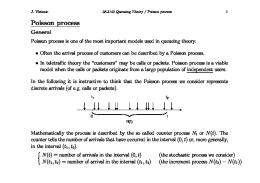
Poisson process is one of the most important models used in queueing theory. •
Often the arrival process of customers can be described by a Poisson process.
biology despite the repeated observation that the clock hypothesis does not ... We introduce a parametric model that relaxes the molecular clock by allowing.
point t0 at the origin and define t0 def. = 0. Xn = tn − tn−1, n ≥ 1, is called the nth
interarrival time. We view t as time and view tn as the nth arrival time. The word ...
PETER EICHELSBACHER AND MA LGORZATA ROOS. Abstract. In the present paper we consider compound Poisson approxima- tion by Stein's method for ...
In this context, the Stein-Chen method for Poisson approximation has proved a ... results of Arratia, Goldstein and Gordon (1989, 1990) using the Stein-Chen.
The two common methods for testing whether software has met its security requirements are functional (Allen,. Barnum, Ellison, McGraw, Mead, 2008) and risk-.
The value of a television was £600 on 1st March 2013. Every four months, the value of the television decreased by 8% of
[Benda and Dunne, 1997; Iida, 2004], water availability [Lettenmaier and ...... 1988; Cowpertwait, 1995; Cowpertwait and O'Connell, 1997; Cowpertwait et al., 2007] .... not available [Vanmullem, 1991; James et al., 1992; Nearing et al., 1996; ...
If you invest P dollars at the annual interest rate r, then after one year the interest
is ... For compound interest, the year is divided into k equal time periods and the.
Solving Compound Interest Problems. What is Compound Interest? If you walk
into a bank and open up a savings account you will earn interest on the money ...
Compound Interest. Dan Saunders. 1 Simple Interest. Given a principal P,
interest rate r, and a time horizon of t periods, we can calculate simple interest as:
.
Jan 5, 2012 - compounds, thus giving researchers a sense of what can be done with them at a molecular level. Clive Morris, AstraZeneca's VP of new ...
Stochastic Interest Model Based on Compound Poisson Process and ...
Apr 30, 2017 - 1 School of Statistics, Qufu Normal University, Qufu, Shandong 273165, China. 2School of Insurance, Shandong University of Finance and ...
Hindawi Mathematical Problems in Engineering Volume 2017, Article ID 3472319, 8 pages https://doi.org/10.1155/2017/3472319
Research Article Stochastic Interest Model Based on Compound Poisson Process and Applications in Actuarial Science Shilong Li,1,2 Chuancun Yin,1 Xia Zhao,3 and Hongshuai Dai4 1
School of Statistics, Qufu Normal University, Qufu, Shandong 273165, China School of Insurance, Shandong University of Finance and Economics, Jinan, Shandong 250014, China 3 School of Statistics and Information, Shanghai University of International Business and Economics, Shanghai 201620, China 4 School of Statistics, Shandong University of Finance and Economics, Jinan, Shandong 250014, China 2
1. Introduction In traditional study of life insurance, interest rate is assumed to be deterministic. However, durations of policies are typically very long (often 20 or even more years) in life insurance and life annuity. So the uncertainty of future interest rate influences the accuracy of its actuarial values deeply. In addition, stochastic models have been widely used in finance and insurance (such as [1–4]). Hence, it is necessary and natural to consider stochastic interest models in life contingencies. So far, many models have been investigated in order to describe the randomness of interest in actuarial literature. Reference [5] first treated the force of interest as a random variable in his actuarial research. In [6], autoregressive models of order one are introduced to model interest rate. References [7, 8] computed moments of insurance and annuity functions using similar models. Reference [9] modeled the force of interest as an ARIMA(𝑝, 𝑑, 𝑞) process and utilized this model to analyze the moments of present value functions. Reference [10] used a Markov process to model the series of interest rates in the research of ruin probability. The above
literatures enriched the application of stochastic interest models in actuarial science, but they assume that the interest rate in one year is fixed, which does not always agree with the practice of financial market. To capture the randomness of interest rates in actuarial science better, the method of stochastic perturbation was proposed. In this method, the interest force at time 𝑡 is expressed as 𝛿𝑡 = 𝛿 + 𝑋 (𝑡) ,
(1)
where 𝛿 is an interest force unrelated to the time 𝑡 and 𝑋(𝑡) denotes a stochastic process resulting in perturbation of fixed interest force 𝛿. Hence, the accumulated interest force function is 𝑡
There are two modeling ways about perturbation methods in actuarial literatures. The first one considers 𝑍(𝑡) as a stochastic process, like Wiener process, Ornstein-Uhlenbeck process, Poisson process, and so on. References [11, 12] constructed stochastic interest rate models regarding 𝑍(𝑡)
2 as Ornstein-Uhlenbeck process and Wiener process, respectively, and investigated the mean and the standard deviation of continuous-time life annuities. Reference [13] studied the mean and the variance of the present value of discrete-time streams in life insurance under these models. Reference [14] also discussed the distribution of life annuities with stochastic interest models driven by Wiener process and OrnsteinUhlenbeck process, respectively. Considering the jumps in interest process, [15, 16] expressed the accumulated force of interest by Wiener process and Poisson process and further studied the optimal dividend strategy in ruin theory and pricing perpetual options, respectively. In the second way, the researchers first describe the perturbation of interest force 𝑋(𝑡) as a special stochastic process and then find the accumulated interest force function by stochastic integration. References [17, 18] discussed the first three moments of homogeneous portfolios of life insurance and endowment policies by modeling the force of interest directly based on the Wiener process or the OrnsteinUhlenbeck process and [19] also generalized these results to heterogeneous portfolios. The stochastic upper and lower bounds on the present value of a sequence of cash flows are discussed in [20]. Reference [21] also introduced a class of stochastic interest model in which the force of interest is driven by second order stochastic differential equation. Reference [22] compared these two approaches to the randomness of interest rates by modeling the accumulated force of interest rate and by modeling the force of interest. Both of these two modeling ways have attracted much attention from researchers. The first way brings convenience to calculation, but the behavior of the force of interest can not be expressed distinctly. In the second way, so far only a few special and simple processes have been considered because of great difficulty to the related stochastic calculations, especially under the case with random jumps. However, the market interest rate often jumps discontinuously and randomly (such as the Federal reserve rate and the China’s central bank benchmark interest rate). Here we introduce a new class of stochastic interest model in which the force of interest is expressed by compound Poisson process directly. This model might characterize the stochastic jumping of market interest rate more honestly and directly. This paper is organized as follows. In Section 2, we give stochastic interest model based on compound Poisson process and further obtain mathematical expectation of present value of the payment paid at a future time point. In Section 3, its properties and applicability are investigated. In Section 4, we discuss actuarial present values of life annuities in discrete and continuous cases. Simulation results show the influences of the parameters on actuarial present values of annuities. In Section 5, we conclude this paper and put forward some interesting problems in the following sequel researches.
2. Stochastic Interest Model under Compound Poisson Process In this section, we construct a new class of stochastic interest models. As a premise, the following assumptions are given:
Mathematical Problems in Engineering (1) the adjustment interarrival times of interest rate are random; (2) the adjustment direction (rise or fall) of interest rate in every stage is independent of each other; (3) the adjustment range of interest rate in every stage is identical. As we know, these assumptions coincide with plenty of practical finance markets. All random variables and stochastic processes under consideration are defined on an appropriate probability space (Ω, 𝑃, F) and are integrable. 2.1. Compound Poisson Process. Compound Poisson process has been widely used in the field of finance and actuarial science, especially in classical ruin probability model. It is described as follows: 𝑁(𝑡)
𝑆 (𝑡) = ∑ 𝑌𝑛 , 𝑡 > 0, 𝑆 (0) = 0,
(3)
𝑛=1
where {𝑁(𝑡), 𝑡 ≥ 0} is a Poisson process with rate 𝜆 > 0 which will indicate the adjustment number of the market interest rate on time interval [0, 𝑡] in this paper. {𝑌𝑛 }∞ 𝑛=1 is a sequence of i.i.d. random variables with common distribution 𝐹(𝑥) = 𝑃(𝑌𝑛 ≤ 𝑥), and {𝑁(𝑡), 𝑡 ≥ 0} and {𝑌𝑛 }∞ 𝑛=1 are independent. Suppose that {𝑋1 , 𝑋2 , . . . , 𝑋𝑛 , . . .} are the interoccurrence times between adjacent adjustments of interest rate; then they are independent and obey exponential distribution with the same parameter 𝜆 > 0. For Poisson process {𝑁(𝑡), 𝑡 ≥ 0}, we first introduce the following important property (see [23]). Lemma 1. Given that 𝑁(𝑡) = 𝑛, the 𝑛 arrival times 𝑇1 , 𝑇2 , . . . , 𝑇𝑛 have the same distribution as the order statistics corresponding to 𝑛 independent random variables uniformly distributed on the interval [0, 𝑡]. That is, the joint density function of 𝑇1 , 𝑇2 , . . . , 𝑇𝑛 is 𝑓 (𝑡1 , 𝑡2 , . . . , 𝑡𝑛 ) =
𝑛! , 0 < 𝑡1 < 𝑡2 < ⋅ ⋅ ⋅ < 𝑡𝑛 ≤ 𝑡. 𝑡𝑛
(4)
From Lemma 1, we usually say that, under condition 𝑁(𝑡) = 𝑛, the times 𝑇1 , 𝑇2 , . . . , 𝑇𝑛 at which events occur, considered as unordered random variables, are distributed independently and uniformly on the interval [0, 𝑡]. 2.2. Stochastic Interest Model under Compound Poisson Process. Suppose that the force of interest {𝛿𝑡 , 𝑡 ≥ 0} is expressed by 𝑁(𝑡)
𝛿𝑡 = 𝛿0 + 𝛼 ∑ 𝑌𝑖 , 𝑡 ∈ [0, +∞) .
(5)
𝑖=1
Here, 𝑌𝑖 (𝑖 = 1, 2, 3, . . .) is the direction of the 𝑖th adjustment of the force of the interest rate with {𝑌𝑖 = 1} for the raise and {𝑌𝑖 = −1} for the reduction. Meanwhile 𝑃(𝑌𝑖 = 1) = 1 − 𝑃(𝑌𝑖 = −1) = 𝑝 (0 ≤ 𝑝 ≤ 1) and {𝑌𝑖 (𝑖 = 1, 2, . . .)} are i.i.d. and also independent of {𝑁(𝑡), 𝑡 ≥ 0}. In this model, the adjustment range of interest force in every change is the same as that denoted by 𝛼.
Figure 1: Representing graph of the integration of 𝐽0𝑡 .
𝑛
+ (1 − 𝑝) (𝑒𝛼𝑡 − 1)] = 𝛽𝑡𝑛 ,
The process {𝛿𝑡 , 𝑡 ≥ 0} is a special continuous-time Markov process, the birth and death process. The initial status of this process is 𝛿0 , and the corresponding birth rate and death rate are 𝑞𝛿𝑡 ,𝛿𝑡 +𝛼 = 𝜆𝑝 and 𝑞𝛿𝑡 ,𝛿𝑡 −𝛼 = 𝜆(1−𝑝), respectively. Substituting formula (5) into (2), we can find corresponding expression of accumulated interest force function. Since the direct integration is extremely difficult, we use another integration technique, changing the integral direction similar to the idea of Stietjes integral. The integration procedure can be understood from Figure 1. Suppose that there are three adjustments of interest rate on the interval [0, 𝑡] and the adjustment times are 𝑇1 , 𝑇2 , and 𝑇3 , respectively. Then the 𝑡 integral ∫0 𝛿𝑠 𝑑𝑠 can be expressed as 𝛿0 𝑡 − 𝛼(𝑡 − 𝑇1 ) + 𝛼(𝑡 − 𝑡
𝑇2 ) + 𝛼(𝑡 − 𝑇3 ). That is, ∫0 𝛿𝑠 𝑑𝑠 = 𝛿0 𝑡 + 𝛼 ∑3𝑖=1 𝑋𝑖 (𝑡 − 𝑇𝑖 ), where 𝑋𝑖 , 𝑖 = 1, 2, 3, show adjustment directions of interest rate. So we can obtain 𝑁(𝑡)
𝐽0𝑡 = 𝛿0 𝑡 + 𝛼 ∑ 𝑋𝑖 (𝑡 − 𝑇𝑖 ) ,
(6)
𝑖=1
where 𝑇𝑖 denotes the time of the 𝑖th adjustment of the force of the interest rate. From formula (6), the random present value of one unit payment at time 𝑡 can be expressed as exp (−𝐽0𝑡 )
𝑁(𝑡)
= exp (−𝛿0 𝑡) ∏ exp (−𝛼𝑋𝑖 (𝑡 − 𝑇𝑖 )) ,
(7)
where random variables, 𝑈1 , 𝑈2 , . . . , 𝑈𝑛 , are distributed independently and uniformly on the interval [0, 𝑡], and 1 [𝑝 (1 − 𝑒−𝛼𝑡 ) + (1 − 𝑝) (𝑒𝛼𝑡 − 1)] 𝛼𝑡 1 = [(𝑒𝛼𝑡 − 1) + 𝑝 (2 − 𝑒−𝛼𝑡 − 𝑒𝛼𝑡 )] . 𝛼𝑡
𝛽𝑡 =
and its mathematical expectation is 𝐸 (exp (−𝐽0𝑡 )) (8)
= exp (−𝛿0 𝑡) 𝐸 ( ∏ exp (−𝛼𝑋𝑖 (𝑡 − 𝑇𝑖 ))) . 𝑖=1
It can be found from the law of total expectation that
𝑝 = 𝑝∗ = =
⋅ 𝐸 (𝐸 ( ∏ exp (−𝛼𝑋𝑖 (𝑡 − 𝑇𝑖 ))) | 𝑁 (𝑡)) . 𝑖=1
exp (𝛼𝑡) − 𝛼𝑡 − 1 exp (𝛼𝑡) + exp (−𝛼𝑡) − 2
exp (𝛼𝑡) (exp (𝛼𝑡) − 𝛼𝑡 − 1) (exp (𝛼𝑡) − 1)
2
(12)
,
we find that 𝛽𝑡 = 1 which means that mathematical expectation of the present value of one unit currency at time 𝑡 will be exp(−𝛿0 𝑡). That is, from the point of view of the mathematical expectation, the randomness of the market interest rate will not have an effect on this present value. Hence 𝑝∗ is called the equilibrium probability at time 𝑡 here. At the same time, the following theorem can be obtained. Theorem 2. The equilibrium probability 𝑝∗ in formula (12) satisfies the following properties:
𝐸 (exp (−𝐽0𝑡 )) = exp (−𝛿0 𝑡) 𝑁(𝑡)
(11)
Based on formula (10), we can find that 𝛽𝑡 is nonincreasing with respect to 𝑝 if 𝛼𝑡 is fixed and satisfies the following properties. (1) If 𝑝 = 0, the market interest will always decrease at the adjusting times of interest rate. Because 𝑒𝛼𝑡 − 1 > 𝛼𝑡, we can find that 𝛽𝑡 = (1/𝛼𝑡)(𝑒𝛼𝑡 − 1) > 1. In this condition, it may happen that the interest rate will be negative if the number of adjusting interest rate times on the interval [0, 𝑡] is large enough. (2) If 𝑝 = 1, the market interest will always increase at the adjusting times of interest rate. Since 1 − 𝑒−𝛼𝑡 < 𝛼𝑡, we have 𝛽𝑡 = (1/𝛼𝑡)(1 − 𝑒−𝛼𝑡 ) < 1. In this condition, the larger the number of adjusting interest rate times on the interval [0, 𝑡] is, the smaller the present value of the currency is. (3) If
𝑖=1
𝑁(𝑡)
(10)
(9)
(1) 𝑝∗ is an increasing function with respect to 𝛼𝑡; (2) 0.5 < 𝑝∗ < 1; (3) lim𝛼𝑡→+∞ 𝑝∗ = 1 and lim𝛼𝑡→0 𝑝∗ = 0.5.
4
Mathematical Problems in Engineering
Proof. Let 𝑦 = 𝛼𝑡 and 𝜙(𝑦) = 𝑒𝑦 (𝑒𝑦 − 𝑦 − 1)/(𝑒𝑦 − 1)2 ; then 𝑝∗ = 𝜙(𝑦). Since 𝜙 (𝑦) = (𝑒𝑦 (𝑒𝑦 −𝑦−1)+(𝑒𝑦 −1))/2(𝑒𝑦 −1) > 0, we can show that 𝜙(𝑦) is a strictly increasing function on 𝑅+ which illustrates that 𝑝∗ is an increasing function with respect to 𝛼𝑡. Further, it is easy to prove that lim𝑦→+∞ 𝜙(𝑦) = 1 and lim𝑦→0+ 𝜙(𝑦) = 0.5. The proof is completed. The following theorem shows the expression of the mathematical expectation of the random present value of one unit currency at time 𝑡 given in formula (8). Theorem 3. Under stochastic interest model (5), the mathematical expectation of the random present value of one unit currency at time 𝑡 can be expressed as 𝐸 (exp (−𝐽0𝑡 ))
= exp (−𝛿0 𝑡 + 𝜆𝑡 (𝛽𝑡 − 1)) .
(13)
Proof. Based on the properties of the condition expectation, it can be obtained by substituting (10) into (9) that 𝐸 (exp (−𝐽0𝑡 ))
Since 𝑓 (0) = 𝛿0 > 0 and lim𝑡→+∞ 𝑓 (𝑡) < 0, there is at least one critical value 𝑡∗ which satisfies 𝑓 (𝑡∗ ) = 0. Now, we will try to find the value of 𝑡∗ . Let us solve the equation (𝛿0 + 𝜆) − 𝜆 [(1 − 𝑝) 𝑒𝛼𝑡 + 𝑝𝑒−𝛼𝑡 ] = 0,
(17)
which can be rearranged to 2
𝜆 (1 − 𝑝) (𝑒𝛼𝑡 ) − (𝛿0 + 𝜆) 𝑒𝛼𝑡 + 𝜆𝑝 = 0.
(18)
Now we investigate the quadratic function 𝑔 (𝑦) = 𝜆 (1 − 𝑝) 𝑦2 − (𝛿0 + 𝜆) 𝑦 + 𝜆𝑝.
(19)
Obviously, 𝑔(0) = 𝜆𝑝 > 0, 𝑔(1) = −𝛿0 < 0, and 𝑔(+∞) → +∞; then two real roots of (19) lie in the interval (0, 1) and the interval (1, +∞), respectively. Because 𝑒𝛼𝑡 > 0 when the condition 𝑡 > 0, we can only consider the root in the interval (1, +∞) which is
= exp (−𝛿0 𝑡 − 𝜆𝑡) ∑
2
∗
𝑦 =
= exp (−𝛿0 𝑡 + 𝜆𝑡 (𝛽𝑡 − 1)) .
(𝛿0 + 𝜆) + √(𝛿0 + 𝜆) − 4𝜆2 𝑝 (1 − 𝑝) 2𝜆 (1 − 𝑝)
∗
= 𝑒𝛼𝑡 ,
(20)
and then the critical value of the interest rate model is 𝑡∗
3. Validity of Stochastic Interest Model
2
Under stochastic interest model (5), we can find that the expected present value of one unit currency at time 𝑡 will be larger than that under fixed force of interest 𝛿0 when 𝑝 = 0.5, and the larger the adjustment frequency intensity of the interest rate, 𝜆, is, the larger the difference between the two above-mentioned values is. That is, when the market interest rate is adjusted frequently, the future interest rate will tend to be underestimated if stochastic interest rate model in formula (5) is considered. This phenomenon often appears in modeling the stochastic interest rate based on a Wiener processes too, such as [11, 12, 17]. If we use 𝛿∗ = 𝛿0 − 𝜆(𝛽𝑡 − 1) as the equivalent force of interest of the stochastic interest model, formula (13) can be expressed equivalently as 𝐸(exp(−𝐽0𝑡 )) = exp(−𝛿∗ 𝑡). 3.1. Validity Condition of Interest Model. In this stochastic model, if 𝑝 < 𝑝∗ , then 𝛽𝑡 > 1; 𝐸(exp(−𝐽0𝑡 )) will be larger than 1 when 𝑡 is large enough, and this is not consistent with the actual situation in most cases. In this section, we will discuss how to restrict the value of the future time in this stochastic interest model. Let 𝑓 (𝑡) = 𝛿0 𝑡 − 𝜆𝑡 (𝛽𝑡 − 1) ;
3.2. Numerical Simulation Analysis. Based on the above 𝑡 analysis, when 𝑡 < 𝑡∗ , the expected present value 𝐸(𝑒−𝐽0 ) is decreasing with respect to investment term 𝑡. That is, only when 𝑡 < 𝑡∗ can the stochastic interest model be used in practice. Figures 2 and 3 show the variation tendency of the critical value with the change of 𝑝 from 0.4 to 0.7 under 𝛿0 = 0.04 and 0.05, respectively, and the curves from top to bottom are based on 𝜆 = 1, 1.5, 2, 2.5, and 3. In Table 1, the critical values 𝑡∗ under different 𝛿0 , 𝜆, and 𝑝 are given. From Figures 2 and 3 or Table 1, the critical value becomes larger and larger with 𝑝 or 𝛿0 increasing. On the contrary, the critical value will decrease if 𝜆 increases. Hence, while using this stochastic interest model, we should consider the values of every parameter and verify whether the term of investment is less than the corresponding critical value. Fortunately, from the actual conditions of adjustments of interest rate in financial markets and ordinary life insurance periods, we find that the critical value 𝑡∗ can satisfy the application condition of this interest rate model in general case.
Mathematical Problems in Engineering
5
Table 1: Critical values 𝑡∗ under different 𝛿0 , 𝜆, and 𝑝. 𝛿0
Figure 2: Values of 𝑡∗ under 𝛿0 = 0.04, 𝛼 = 0.0025, and 𝜆 = 1, 1.5, 2, 2.5, 3, respectively.
4. Life Annuities under Stochastic Interest Model Following the notations in [24], the symbol (𝑥) is used to denote a life-age-𝑥. The future lifetime and the curtate-futurelifetime of 𝑥 are denoted by 𝑇(𝑥) and 𝐾(𝑥), respectively. 4.1. Actuarial Present Values for Discrete Life Annuities. There are two classes of the discrete life annuities: the discrete life annuities-due and the discrete life annuities-immediate. First of all, we consider the former. In the nomenclature, an annuity is called a whole life annuity-due if the annuity pays a unit amount at the beginning of each year that the annuitant (𝑥) survives, and the actuarial present value of the annuity can be expressed as +∞ 𝑘=0
0.7
0.75
Figure 3: Values of 𝑡∗ under 𝛿0 = 0.05, 𝛼 = 0.0025, and 𝜆 = 1, 1.5, 2, 2.5, 3, respectively.
where 𝑃(𝐾(𝑥) = 𝑘) = 𝑘| 𝑞𝑥 = 𝑘 𝑝𝑥 ⋅𝑞𝑥+𝑘 in actuarial theory and according to interest theory, we have 𝑘
𝑛
𝑘
𝑛
̈ = 𝐸 ( ∑ 𝑒− ∫0 𝛿𝑡 𝑑𝑡 ) = ∑ 𝐸 (𝑒−𝐽0 ) 𝑎𝑘+1| 𝑛=0
̈ 𝑃 (𝐾 (𝑥) = 𝑘) , ̈ 𝑎𝑥̈ = 𝐸 (𝑎𝐾(𝑥)+1| ) = ∑ 𝑎𝑘+1|
0.65
p value
𝑛=0
(23) 𝑘
= ∑ 𝑒−𝛿0 𝑛+𝜆𝑛(𝛽𝑛 −1) . 𝑛=0
Combining formula (22) with formula (23), we obtain the following formula under stochastic interest model introduced here: +∞
(22)
𝑎𝑥̈ = 1 + ∑ 𝑒−𝛿0 𝑛+𝜆𝑛(𝛽𝑛 −1) 𝑛 𝑝𝑥 . 𝑛=1
(24)
6
Mathematical Problems in Engineering ̈ Table 2: Values of 𝑎30:30| for different 𝛿0 , 𝛼, 𝜆, and 𝑝 under the stochastic interest rate model.
The procedures used above for annuities-due can be adapted for annuities-immediate where payments are made at the ends of the payment periods. Such that, for a whole life annuity-immediate, the actuarial present value can be given as +∞
−𝛿0 𝑛+𝜆𝑛(𝛽𝑛 −1)
𝑎𝑥 = ∑ 𝑒 𝑛=1
𝑛 𝑝𝑥 ,
(26)
and the actuarial present value of 𝑛-year temporary life annuity for the annuitant (𝑥) is 𝑛
𝑎𝑥:𝑛| = ∑ 𝑒−𝛿0 𝑘+𝜆𝑘(𝛽𝑘 −1) 𝑘 𝑝𝑥 .
(27)
𝑘=1
Using Fubini’s theorem, from formulas (28), we have +∞
𝑎𝑥 = ∫
0
+∞
𝑎𝑥 = 𝐸 (𝑎𝑇(𝑥)| ) = ∫
0
𝑎𝑡| 𝑑𝐹𝑇(𝑥) (𝑡) ,
(29)
Substituting formula (13) into formula (29), we have +∞
𝑎𝑥 = ∫
0
exp (−𝛿0 𝑡 + 𝜆𝑡 (𝛽𝑡 − 1)) 𝑡 𝑝𝑥 𝑑𝑡,
(30)
and then the actuarial present value of an 𝑛-year temporary continuous life annuity for the annuitant (𝑥) is 𝑛
𝑎𝑥:𝑛| = ∫ exp (−𝛿0 𝑡 + 𝜆𝑡 (𝛽𝑡 − 1)) 𝑡 𝑝𝑥 𝑑𝑡. 0
4.2. Actuarial Present Value for Continuous Life Annuities. In order to analyze the actuarial present value of this class of annuities, we first consider the whole life annuity payable continuously at the rate of 1 per year. For an annuitant (𝑥), the actuarial present value of this life annuity is denoted by 𝑎𝑥 . From [24], we can obtain the following formula:
𝐸 (exp (−𝐽0𝑡 )) 𝑡 𝑝𝑥 𝑑𝑡.
(31)
4.3. Numerical Analysis. Based on the results in Sections 4.1 and 4.2, we calculate the actuarial present value of both a 30-year temporary discrete life annuity-due and a 30year temporary continuous life annuity for the annuitant (30) under different 𝛿0 , 𝛼, 𝜆, and 𝑝. The simulation results are shown in Tables 2 and 3, respectively. In these calculations, the experience life table of the Chinese life insurance (2000–2003) (male) is used. It should be noted that the
Mathematical Problems in Engineering
7
Table 3: Values of 𝑎30:30| for different 𝛿0 , 𝛼, 𝜆, and 𝑝 under the stochastic interest rate model. 𝛿0
Uniform Distribution assumption—the classical fractional age assumption—is used in the calculation of the actuarial present values of the continuous life annuity. From Tables 2 and 3, we can find that the actuarial present values become smaller and smaller as the probability that the interest rate rises at the change time point, 𝑝, increases continuously when other parameters are fixed and this result is obvious because the probability of the future force of interest rising will become larger and larger with 𝑝 increasing. Furthermore, all the values when 𝑝 = 0.5 are larger than those under the nonrandom condition (i.e., 𝛿𝑡 ≡ 𝛿0 for 𝑡 ≥ 0), which verifies Theorem 2 from the quantitative aspect. At the same time, under the condition that 𝛿0 , 𝛼, and 𝑝 are fixed, the actuarial present value becomes larger and larger with increasing 𝜆, and this result illustrates that the present value will increase if the interest rate changes frequently. If other conditions are fixed, the actuarial present value also becomes larger and larger with increasing 𝛼 which means that the present value will increase if the range of every interest rate change is larger. At last, we can find that the actuarial present value will become larger with decreasing 𝛿0 which verifies that the present value of the money at future time will decrease in general if the initial interest rate increases in practice.
15.2396
process directly. Different from the references, the modeling method makes the interest model more reasonable and the random jumping behavior of interest rate is described directly. We investigate the validity conditions of this model and introduce a conception called the critical value of the interest rate model. Based on this model, several common life annuities are studied and the numerical results under different parameters are compared adequately. This paper proposes a new research perspective of modeling stochastic interest. Following this idea, there are several meaningful issues which deserve to study further. (1) Some continuous stochastic processes can be blended into modeling stochastic interest rate on the basis of the model in this paper. (2) This model can be generalized by using some random variables for the change ranges of the force of interest and for the frequency parameter of the Poisson process in this model. (3) Both the empirical study and the statistical analysis about this stochastic interest rate should be made. We will explore these issues in our future researches.
Conflicts of Interest The authors declare that they have no conflicts of interest.
Acknowledgments 5. Conclusion In this paper, we introduce a new stochastic interest model in which the force of interest is driven by compound Poisson
This work was partially supported by NSFC (11571198 and 71671104), Project of Humanities and Social Sciences of MOE, China (16YJA910003), Project of Shandong Province Higher
8 Educational Science and Technology Program (J15LI01), Special Funds of Taishan Scholars Project of Shandong Province, and Incubation Group Project of Financial Statistics and Risk Management of SDUFE.
References [1] S. Tiong, “Pricing inflation-linked variable annuities under stochastic interest rates,” Insurance: Mathematics and Economics, vol. 52, no. 1, pp. 77–86, 2013. [2] K. Buchardt, “Dependent interest and transition rates in life insurance,” Insurance: Mathematics and Economics, vol. 55, no. 1, pp. 167–179, 2014. [3] Y. Jin and S. Zhong, “Pricing spread options with stochastic interest rates,” Mathematical Problems in Engineering, vol. 2014, Article ID 734265, 11 pages, 2014. [4] M. Joshi and N. Ranasinghe, “Non-parametric pricing of longdated volatility derivatives under stochastic interest rates,” Quantitative Finance, vol. 16, no. 7, pp. 997–1008, 2016. [5] J. H. Pollard, “On fluctuating interest,” Bulletin van de Koniniklijke Vereniging Van Belgische Actuarissen, vol. 66, pp. 68–97, 1971. [6] P. P. Boyle, “Rates of return as random variables,” The Journal of Risk and Insurance, vol. 43, no. 4, pp. 693–711, 1976. [7] H. H. Panjer and D. R. Bellhouse, “Stochastic modelling of interest rates with applications to life contingencies,” The Journal of Risk and Insurance, vol. 47, no. 1, pp. 91–110, 1980. [8] D. R. Bellhouse and H. H. Panjer, “Stochastic modelling of interest rates with applications to life contingencies. part II,” The Journal of Risk and Insurance, vol. 48, no. 4, pp. 628–637, 1981. [9] J. Dhaene, “Stochastic interest rates and autoregressive integrated moving average processes,” Astin Bulletin, vol. 19, no. 2, pp. 131–138, 1989. [10] J. Cai and D. C. M. Dickson, “Ruin probabilities with a Markov chain interest model,” Insurance: Mathematics and Economics, vol. 35, no. 3, pp. 513–525, 2004. [11] J. A. Beekman and C. P. Fuelling, “Interest and mortality randomness in some annuities,” Insurance Mathematics and Economics, vol. 9, no. 2-3, pp. 185–196, 1990. [12] J. A. Beekman and C. P. Fuelling, “Extra randomness in certain annuity models,” Insurance Mathematics and Economics, vol. 10, no. 4, pp. 275–287, 1992. [13] J. De¸bicka, “Moments of the cash value of future payment streams arising from life insurance contracts,” Insurance: Mathematics and Economics, vol. 33, no. 3, pp. 533–550, 2003. [14] T. Hoedemakers, G. Darkiewicz, and M. Goovaerts, “Approximations for life annuity contracts in a stochastic financial environment,” Insurance: Mathematics and Economics, vol. 37, no. 2, pp. 239–269, 2005. [15] X. Zhao and B. Zhang, “Pricing perpetual options with stochastic discount interest rates,” Quality and Quantity, vol. 46, no. 1, pp. 341–349, 2012. [16] X. Zhao, B. Zhang, and Z. Mao, “Optimal dividend payment strategy under Stochastic interest force,” Quality and Quantity, vol. 41, no. 6, pp. 927–936, 2007. [17] G. Parker, “Moments of the present value of a portfolio of policies,” Scandinavian Actuarial Journal, vol. 1994, no. 1, pp. 53– 67, 1994. [18] G. Parker, “Stochastic analysis of a portfolio of endowment insurance policies,” Scandinavian Actuarial Journal, vol. 1994, no. 2, pp. 119–130, 1994.
Mathematical Problems in Engineering [19] G. Parker, “Stochastic analysis of the interaction between investment and insurance risks,” North American Actuarial Journal, vol. 1, no. 2, pp. 55–84, 1997. [20] H. Cossette, M. Denuit, J. Dhaene, and E. Marceau, “Stochastic approximations of present value functions,” Bulletin of the Swiss Association of Actuaries, vol. 1, pp. 15–28, 2001. [21] G. Parker, “A second order stochastic differential equation for the force of interest,” Insurance Mathematics and Economics, vol. 16, no. 3, pp. 211–224, 1995. [22] G. Parker, “Two stochastic approaches for discounting actuarial functions,” ASTIN Bulletin, vol. 24, no. 2, pp. 167–181, 1994. [23] S. M. Ross, Stochastic Processes, John Wiley & Sons, Inc, New York, NY, USA, 2nd edition, 1996. [24] N. L. Bowers, H. U. Gerber, J. C. Hickman, D. A. Jones, and C. J. Nesbitt, Actuarial Mathematics, The Society of Actuaries, Ill, USA, 2nd edition, 1997.
Advances in
Operations Research Hindawi Publishing Corporation http://www.hindawi.com