local search for constraint optimisation problems. 1 Introduction ... service is maximised.1 The first scenario corresponds to minimising the span while the ...... Coloring graphs with a general heuristic search engine. In Johnson et al. [29], pages ...
Stochastic Local Search Algorithms for Graph Set T -Colouring and Frequency Assignment Marco Chiarandini∗ University of Southern Denmark, IMADA, Odense, Denmark Thomas St¨ utzle Universit´e Libre de Bruxelles, CoDe, IRIDIA, Brussels, Belgium
Abstract The graph set T -colouring problem (GSTCP) generalises the classical graph colouring problem; it asks for the assignment of sets of integers to the vertices of a graph such that constraints on the separation of any two numbers assigned to a single vertex or to adjacent vertices are satisfied and some objective function is optimised. Among the objective functions of interest is the minimisation of the difference between the largest and the smallest integers used (the span). In this article, we present an experimental study of local search algorithms for solving general and large size instances of the GSTCP. We compare the performance of previously known as well as new algorithms covering both simple construction heuristics and elaborated stochastic local search algorithms. We investigate systematically different models and search strategies in the algorithms and determine the best choices for different types of instance. The study is an example of design of effective local search for constraint optimisation problems.
1
Introduction
The graph set T -colouring problem (GSTCP) is a generalisation of the graph (vertex) colouring problem (GCP) that was introduced to model the assignment of frequencies to radio transmitters [22]. In the GSTCP, one is given a graph, a number of colours required at each vertex and separation constraints for each vertex and for each pair of connected vertices. Colours correspond to nonnegative integers and the separation constraints represent the disallowed differences between the integers assigned to each vertex. The decision version of the GSTCP asks, given a number of colours, for an assignment of sets of ∗
Corresponding author.
1
colours to the vertices of the graph such that all constraints are satisfied. Such an assignment is called a set T-colouring. There are various optimisation versions of the GSTCP, which differ in the objective function to be minimised [22, 49]. One version asks to determine the T -order (or T -chromatic number), that is, the minimal number of integers, such that a set T -colouring exists. A second optimisation version asks to determine the T -span, that is, the minimal difference between the largest and the smallest integers such that a set T -colouring exists. Another alternative, sets a bound on the number of available colours and asks for a set T -colouring that minimises the number of constraint violations. The GSTCP is at the core of a number of real-world applications. Examples are traffic phasing, fleet maintenance [44] and task assignment. In this latter case, a large task is divided into incompatible subtasks (for example, due to resource conflicts) and the problem is to assign a set of time periods to each subtask such that incompatible subtasks are treated in different time periods [49]. The most important GSTCP application is in the assignment of frequencies to radio transmitters. In this case, vertices represent transmitters and colours the frequencies to be assigned to the transmitters subject to certain interference constraints, the T -constraints [22]. These T -constraints are expressed in the form of restrictions on the possible separations of the frequencies at each vertex and between the vertices. In the frequency assignment application, there are two possible scenarios of interest: the design scenario, in which it has to be decided which frequency band to acquire in order to satisfy a forecast network utilisation; and the planning scenario, in which the frequency band available at the provider is fixed and it must be decided which frequencies to assign to each cell such that the service is maximised.1 The first scenario corresponds to minimising the span while the second scenario to minimising the number of violated constraints. In this latter case, penalties can then be associated to disallowed separations and acceptable interferences are weighted differently from forbidden interferences. This gives rise to the minimal interference problem, where the total penalty has to be minimised [1, 17]. As we will see, most of the solution methods discussed in this article are valid for both scenarios. Indeed, following a known practice in the constraint satisfaction community [36], the minimal span problem can be approached by solving a series of minimal interference problems. The GSTCP has received significant attention from both the theoretical and the algorithmic perspective. The theoretical contributions often focus on special types of instances and provide results that might be roughly grouped into three classes: computational complexity [44, 49, 20, 21], lower bounds [2, 28, 47, 37] and approximation schemes [45, 27].2 1
Both cases of frequency assignment give rise to what is called, more precisely, the fixed channel assignment problem, whose name is used to emphasise that the model is static, i.e., the set of connections remains stable over time. 2 Theoretically driven research on the GSTCP was also the target of the DI-
2
The algorithmic contributions on the GSTCP are mostly linked to the research on frequency assignment and, more recently, to the “Computational Challenge on Graph Colouring and its Generalisations”, which was organised by Johnson, Mehrotra and Trick.3 The problem is also relevant to the constraint satisfaction community [15] although little experimental research has been conducted on constraint programming models [52]. Mathematical programming approaches are instead described in [17, 1]. However, complete search algorithms have proven to be inefficient when applied to general and large scale instances, which are more of interest for practical applications. Stochastic local search (SLS) algorithms, although incomplete, obtain typically much better quality solutions that the complete algorithms in practicable times and, hence, have also been more studied. Costa is the first to address the GSTCP by means of heuristics and proposes a generalisation of the DSATUR heuristic for the GCP [12]. Dorne and Hao apply tabu search to very large, randomly generated GSTCP instances [16]. In the context of the COLOR02/03/04 DIMACS challenge, Phan and Skiena devised a simulated annealing algorithm using their general-purpose platform Discropt [39]. Prestwich presented a randomised backtracking algorithm [42] while Lim et al. designed a squeaky wheel algorithm [31, 32]. This latter approach also gives the best results for the benchmark instances that were proposed in the COLOR02/03/04 DIMACS challenge. However, from the published results it is unclear how this algorithm compares with the earlier proposed tabu search algorithm by Dorne and Hao [16]. In general, we noted a tendency in this area to publish horse-race type papers that present new best performing algorithms but rarely compare them directly or study the algorithm components that determine the success. The main contribution of this article is a systematic study of previously known and new construction heuristics as well as advanced SLS algorithms for the GSTCP, with the goal to bring instructive insights into the design and implementation of efficient local search algorithms for this constraint optimisation problem. We have decided to (re)-implement all the algorithms using the same framework, data structures, platform and implementer’s ability to increase the fairness of the experimental comparison. Our benchmark collection comprises several sets of randomly generated instances including random graphs and geometric graphs as well as instances derived from the frequency assignment literature [3]. As a side product, we also extend the set of previously available benchmark instances to allow for a more systematic study of the influence of instance features on performance. The experiments are designed in a way to bring light on the sources of differences rather than only indicating which is the best algorithm. Our analysis, supported by statistical MACS/DIMATIA/Renyi Working Group on Graph Colourings and their Generalizations; see (Last update: January 10, 2005) for more details. 3 M. Trick. “Computational Series: Graph Coloring and its Generalizations.”, 2002, . In this challenge, the GSTCP is called bandwidth multi-colouring problem.
3
methods, allows us to investigate (i) which are the key algorithmic features that are responsible for the good performance of the construction heuristics and SLS algorithms, (ii) which are the features of the instances that have an influence on the results and, (iii) which is the current state-of-the-art in GSTCP solving. We draw two kinds of conclusions. The first is of general character and consists of indications about modelling constraints in local search. Perhaps the most remarkable is the fact that we found it helpful to use constraints to reduce the search space size. Although this might be intuitively clear in the constraint satisfaction community, previous results have shown that some sort of constraints, like those for symmetry breaking, may have a negative effect on the performance of local search algorithms [43]. Another indication worth mentioning is that we found convenient solving constrained optimisation problems as a series of constraint satisfaction problems with bounded objective is more convenient than using a weighted sum of optimisation objective and infeasibility. The second kind of conclusions concern specifically the GSTCP. We show that the best construction heuristic for this problem is a generalisation of DSATUR that chooses vertices in a different order to that proposed in previous researches and that the best performing SLS algorithms are a squeaky wheel algorithm and a new tabu search algorithm with a novel randomised exact search neighbourhood. The paper is organised as follows. Section 2 introduces the notation and provides some basic results. Section 3 defines the benchmark instances. Section 4 describes construction heuristics which are empirically assessed in Section 5. Section 6 is dedicated to the description of the SLS algorithms. Section 7 reports the experimental analysis on SLS algorithms. Finally, Section 8 resumes the results of this work.
2
Definitions, Notation and Basic Results
The GSTCP is defined by (i) an undirected graph G = (V, E), where V is the set of vertices and E ⊆ V × V is the set of edges, with uv representing an edge in E; (ii) a set of integers (called colours) Γ; (iii) a number r(v) of required colours for each vertex v ∈ V ; and (iv) a collection T of sets (called T-sets), such that there is a set Tuv for each edge uv ∈ E and a set Tu for each vertex u ∈ V . The T-sets are sets of nonnegative integers and represent the disallowed separations of colours between and within vertices, respectively. The task in the decision version of the GSTCP is to find, for a given number of k = |Γ| colours, a mapping ϕ : V 7→ P(Γ) such that the three following
4
groups of constraints |ϕ(v)| = r(v) |x − y| 6∈ Tu |x − y| 6∈ Tuv
∀v∈V
(1)
∀u ∈ V, ∀x, y ∈ ϕ(u), x 6= y ∀uv ∈ E, ∀x ∈ ϕ(v), ∀y ∈ ϕ(u)
(2) (3)
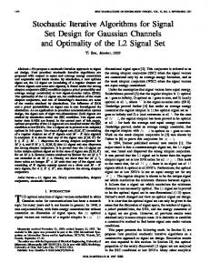
are satisfied. The three groups of constraints are called requirement constraints, vertex constraints, and edge constraints, respectively. We call a mapping ϕ a proper set T-colouring if all constraints are satisfied and improper, otherwise. The graph T -colouring problem (GTCP) is a special case of the GSTCP, with r(v) = 1 for all v in V and only the edge constraints are present. Both, the decision versions of the GSTCP and the GTCP are obviously in N P and, hence, also N P-complete, since they are generalisations of the k-colouring problem [19]. Any GSTCP instance defined by a graph G = (V, E), a collection T and vertex requirements r(v) for each v ∈ V has an equivalent GTCP instance GS = (V S , E S ) such that the existence of a proper T -colouring in the GTCP instance implies that there exists a proper set T-colouring in the GSTCP instance (and vice versa). The equivalence is shown by the construction of the GTCP instance. GS is obtained from G by creating P a vertex u forS each S requirement of a vertex v ∈ V (G) such that |V | = v∈V r(v). In G , the vertices u ∈ V S derived from a vertex v ∈ V form a clique of order r(v) in which each edge receives the set of constraints Tv ∈ T . Every such vertex is then connected with each vertex of the clique induced by another vertex w ∈ V , if vw ∈ E. The colour separation associated with these edges is Tvw . The graph GS is called split graph. Two properties of a proper (set) T -colouring ϕ are of interest for its quality: the order, i.e., the number of different colours effectively used by ϕ and the span, i.e., the maximal difference between the colours used: maxu,v∈V {|x − y| : x ∈ ϕ(v), y ∈ ϕ(u)}. The minimum order for which a proper T -colouring exists is called the (set) T -chromatic number χT (G); the minimum span is the (set) T-span spT (G). Minimising the order, the span or both is the objective in the optimisation versions of the GSTCP. For all graphs G and T -sets T it holds that χT (G) ≤ spT (G) [22]. Note that χT (G) = χT (GS ) and spT (G) = spT (GS ) and, hence, the solution to a GSTCP can be found by solving the GTCP on the split graph. For the GTCP, it was proved that the T -chromatic number of a graph G, χT (G), is equal to the chromatic number χ(G) [13]. However, Hale (1980) [22] pointed out that minimising the span of a T -colouring is different from minimising the order, or the span of a colouring without the T -constraints. There are cases, indeed, where no optimal span T -colouring gives an optimal order and vice-versa. For example, if the graph G and the T-set T are those of Figure 1, then χT (G) = 3 and spT (G) = 3 but a T -colouring with order three
5
(a) The original instance.
(b) A solution with 3 colours and span 4.
(c) A solution with 4 colours and span 3.
Figure 1: A GTCP instance with χT (G) = 3 and spT (G) = 3 (a). Every solution that uses 3 colours has span at least 4 (b), whereas every solution with span 3 uses 4 colours (c).
has span at least four, whereas a T -colouring with span three has order at least four. For the frequency assignment application, more relevant is the case in which all Tu , Tuv ∈ T consist of consecutive integers {0, 1, . . . , tuv − 1} for all uv ∈ E and {0, 1, . . . , tu − 1} for all u ∈ V . This particular version of the problem is known as separation distance GSTCP and the values tu , tuv are called colour distances [17]. The edge and vertex constraints then have the form |x − y| ≥ t, where x and y are two assigned integers. In the rest of the article we assume the GSTCP to be in the separation distance form and study the minimisation of the set T-span. In each set Tcolouring instance we assume minu∈V {x : x ∈ ϕ(u)} = 1 and, hence, the set T-span to be k − 1, where k is the largest colour used. In addition, we denote by AG (v) the set of vertices adjacent to a vertex v ∈ V , i.e., AG (v) = {u|u ∈ V, uv ∈ E}, and by d(v) the degree of a vertex v, i.e., |AG (v)|.
3
Benchmark instances
We use a benchmark suite composed of three sets of random instances that differ in the structure of the graphs and of the constraints, and a set of instances derived from the frequency assignment application. Random geometric instances. This set was proposed by M. Trick in the context of the “Computational Challenge on graph colouring and its generalisations”. Vertices correspond to points that are uniformly distributed in a square [10, 000 × 10, 000]. Edges connect vertices whose corresponding points are closer than some pre-defined value. The separation distances associated to edges are inversely proportional to the distances between the points. Vertex requirements are chosen uniformly at random from the set {1, . . . , r} and vertex separation distances are fixed to 10. The size of these instances ranges from 20 to 120 vertices. We denote this set by GEOM, its class of sparse instances by GEOMn and its classes of denser instances by GEOMna and GEOMnb. The 6
instances GEOMnb have higher requirements per node than GEOMna. Statistics of this instance set are given in Table 1a. Random uniform instances. This set was introduced by Dorne and Hao for testing their tabu search algorithm [16]. The graphs are uniform, random graphs, which are typically identified as Gnp , where n is the number of vertices � and each of the n2 possible edges is included in the graph with a probability p. Vertex requirements, vertex-distances and edge-distances are generated according to a uniform distribution in the interval {1, . . . , t}. Statistics on these instances are in Table 1b. We call this set HD-RU and maintain P the original nomenclature for the single instances: essai.n.R.p where R = r(v) = |V S |. Random uniform instances (new). Since we experienced that some of the HD-RU instances require very high computational times before it becomes unlikely for the algorithms here studied to further improve their solutions, we generated a new set of instances that are similar to those of HD-RU. The only difference is that vertex requirements are chosen uniformly at random from the interval {1, . . . , r}, thus, possibly, r 6= t. The values considered for the parameters and the number of instances generated are reported in Table 1c. The smaller instance size with respect to the set HD-RU allows us to run extensive computational tests. We denote this set of instances NRU and each single class as TG-n-p-r.t. Philadelphia instances. This set comprises the well-known Philadelphia instances from the frequency assignment literature [3]. Vertices correspond to 21 hexagons representing the cells of a cellular phone network. Edges and separation distances are assigned according to the interferences between sites such that adjacent or close cells have higher separation constraints than distant cells. For details on the generation of these instances we refer to the FAP web repository.4 In conformity with the frequency assignment literature, we denote these instances by P1–P9.
4
Construction Heuristics
Construction heuristics are the fastest methods to generate good quality solutions for optimisation problems. Another main use is to provide good initial solutions to SLS algorithms. For the GSTCP, various construction heuristics have been presented. The most comprehensive study so far by Hurley et al. comprises a number of different sequential heuristics [26]. They conclude that it is difficult to predict which variant will perform best on a specific instance; however, their comparison is limited to small size instances of around 20 vertices and no statistical analysis is applied to support the results. 4
A. Eisenbl¨ atter and A. Koster. “FAP web – A website devoted to frequency assignment”. June 2000. . (Last update: January 2007.)
7
|V | 20, 30, . . . , 120
ρ¯ 0.1 0.2
r 3 10 3 10
tu 10 10 10 10
tuv 4.5 4.5 4.5 4.5
# instances – 11 (GEOMn ) 11 (GEOMna) 11 (GEOMnb)
(a) Random geometric instances |V | 30, 100, 300, 500, 1000
p 0.1 0.5 0.9
r = tu = tuv 5 5 5
# instances 5 5 5
(b) Random uniform instances [16]
|V | 60
p 0.1
r 5
0.5
10 5
0.9
10 5 10
t 5 10 5 5 10 5 5 10 5
# instances 10 10 10 10 10 10 10 10 10
Inst P1 P2 P3 P4 P5 P6 P7 P8 P9
(c) New random uniform instances
ρ¯ 0.73 0.49 0.73 0.49 0.73 0.49 0.73 0.73 0.73
[rmin ; rmax ] [8;77] [8; 77] [5; 45] [5; 45] [20; 20] [20; 20] [16; 154] [8; 77] [32; 308]
tu 5 5 5 5 5 5 5 5 5
max [tmin uv ; tuv ] [1; 2] [1; 2] [1; 2] [1; 2] [1; 2] [1; 2] [1; 2] [1; 2] [1; 2]
(d) Philadelphia instances
Table 1: Statistics on the benchmark instances. tu and tuv are used explicitely if the range of values differs among vertex and edge constraints. ρ¯ gives the measured edge density of the graphs.
We enlarge the study of construction heuristics for the GSTCP to include in addition the assignment heuristics proposed in [46] and heuristics that were adapted from the GCP. Some of the proposed heuristics are new, like the adaption of RLF, or are enhancements of previously published ones, like generalised DSATUR.
4.1
Split Graph (T -Colouring) Approach
Sequential heuristics. Sequential heuristics iteratively assign colours to vertices until a complete colouring is reached. Each assignment decision consists of two steps: first, the vertex that is to be coloured next is chosen, then a colour is assigned to this vertex. A basic heuristic to assign the colour is the greedy algorithm [13]. This algorithm, which we denote T-greedy, takes as input a permutation π of the vertices. At each iteration i, it assigns to the vertex π(i) the colour corresponding to the smallest possible integer such that the partial T -colouring obtained after colouring the vertex π(i) remains proper. After |V S | iterations, T-greedy returns a proper complete T -colouring for any graph and T -sets. An efficient implementation of T-greedy maintains a set of forbidden colours for each vertex that is still to be coloured and updates it at each iteration. The
8
complexity is O(k|V S |); note that k is not bounded by the number of vertices. The permutation π can be determined in a static manner before assigning the colours. As in the GCP, the vertex degree is the information which is used to order the vertices. We examine the following orders: Random (RO algorithm), Largest First (LF algorithm) and Smallest Last (SL algorithm). The LF algorithm sorts the vertices in non-increasing order of their degree. The SL algorithm arranges the vertices such that the vertex at position i, vπ(i) has the smallest degree in the subgraph G0 ⊂ G induced by V 0 = {vπ(1) , vπ(2) , . . . , vπ(i) }. This sequence is determined starting at the final vertex and proceeding in reverse order. We denote the three heuristics G-ROS, G-LFS, and G-SLS. Various authors have tested an adjusted vertex degree that uses the additional information of the separation P distance constraints between adjacent T vertices, which is defined as d (v) = u∈AG (v) tuv . We therefore include in our analysis for all the sequential heuristics two versions, one using the vertex degree and another using the adjusted vertex degree. Generalised DSATUR heuristics. The DSATUR heuristics are also based on T-greedy but they generate the order of the vertices in a dynamic manner at construction time depending on the current partial colouring. The information used is the vertex saturation degree, i.e., the number of different colours forbidden at the current vertex by the colours assigned to the adjacent vertices. We denote this generalisation of the DSATUR scheme to the GTCP as G-DSATUR and study the instantiation of its components. We examine two sorting strategies: largest saturation first (LSF) and smallest saturation first (SSF). In both cases, ties are broken by the largest vertex degree. As for the sequential heuristics, we also examine the use of an adjusted vertex degree to break ties. We observed, however, that ties occur very rarely. In addition, we consider a modification of the T-greedy algorithm that selects, whenever more than one previously used colour is feasible, the colour that is feasible for the smallest number of uncoloured vertices. The idea is to favour the use of colours with less chances to be used later in the process. We denote this algorithm as T-greedy# . Its worst case complexity when applied to a static vertex order is O(k 2 |V S |2 ). Empirical observations showed that even for high density graphs with ρ(G) = 0.9, where vertices are less likely to be colourable with previously used colours, this rule applies in about 50% of the decisions taken. Generalised RLF heuristic. For the GCP, one of the best performing construction heuristics, the Recursive Largest First (RLF) heuristic, is based on a partitioning approach. It iteratively fills colour classes by colouring as many vertices as feasible with the same colour before using a new colour. When applied to the GTCP, the concept of independent set is still valid but vertices are also subject to distance constraints and, hence, their insertion in a 9
set must also guarantee the satisfaction of the separation constraints between the colours that will be assigned to such sets. We denote this adapted RLF heuristic by G-RLF. For G-RLF, we also study the effect of an adjusted vertex degree.
4.2
Original Graph (Set T -Colouring) Approach
Sequential heuristics. The T-greedy algorithm can be modified to assign at each construction step r(v) colours to a vertex v. The colour assignment policy remains the same: priority is given to the smallest possible colours. The order of the vertices can be determined using the same rules (RO, LF, SL) as before. We implemented these heuristics using both the vertex degree and the adjusted vertex degree. Assignment heuristics. The heuristics proposed by Sivarajan et al. [46] look at the problem from an assignment perspective. These heuristics were only studied on instances with 21 vertices and never compared with the heuristics introduced above. They work at the level of single vertex requirements. First the requirements are disposed in a matrix of size |V |×maxv∈V r(v) whose rows correspond to vertices and the elements of each row to cyclically shifted versions of the list {1, . . . , r(v)} and zeros. The cylic shifts are organised in such a way that the number of requirements is almost equally distributed among the columns. Then an order in the examination of the matrix is decided and the colours are assigned to the requirements in the order they are visited. Three factors influence the heuristic procedure: the vertex order (i.e., the order of the rows in the matrix) determined by the smallest last (C) or the largest first (D) order of an adjusted vertex degree; the requirement order (i.e., the order of examination in the matrix) determined by row-wise ordering (R) or column-wise ordering (C); and the assignment policy which may be colour exhaustive (F) if we assign the smallest colour that does not introduce any violation to the next requirement, or requirement exhaustive (R) if for each colour in order from 1 to k we scan all yet uncoloured requirements and assign the current colour to all those for which it is feasible. We identify these assignment heuristics by the letter abbreviations as defined above. For example, CRR refers to a heuristic that uses smallest last vertex order, row-wise requirement order and an requirement exhaustive assignment policy.
5
Experimental Assessment of Construction Heuristics
The experimental study on construction heuristics aims at identifying the algorithmic features that have an impact on the heuristics’ performance and the best performing construction heuristics. In fact, the attempt to distinguish and separate the effects of the single choices that compose the heuristics is a 10
RLF
T -colouring approach order={RO,LF,SL} adjust={yes,no} adjust={yes,no},order={LSF,SSF}, assign={T-greedy,T-greedy# } adjust={yes,no}
Assignment
–
Sequential DSATUR
set T -colouring approach order={RO,LF,SL} adjust={yes,no} – – order={C, D},requ.={R, C}, assign={F, R}
Table 2: Implementation choices for the construction heuristics for GSTCP.
novelty of this analysis which is made possible by a careful organisation and design of experiments. Some of these choices are, for example, the use of the GSTCP formulation or the GTCP transformation or the use of an adjusted vertex degree. Concerning performance, we focus uniquely on the solution quality returned by the heuristics since for all heuristics, the computational times are negligible being always below 0.15 seconds on our computer, a 2 GHz AMD Athlon MP 2400+ processor with 256 KB cache and 1GB RAM.5 The different algorithmic choices, whose effects we want to examine, are described in Table 2. We need to split the analysis into four separate experimental designs, one for each type of approach, that is, one for each row of the table. We want to distinguish main and interaction effects of the algorithmic factors and of other factors, such as the instance type. This latter effect tells us how the relative performance of the algorithms depends on some features of the instance that can be recognised a-priori. We use the classes of instances taken from the GEOM and NRU benchmark sets. In addition, we treat the single instances as blocking factor. Since randomised decisions may occur due to random tie breaking, we collect for each heuristic 10 runs per instance and measure the span returned in each run. Then we rank these results for each instance to avoid problems due to different instance scales. Sequential Heuristics. We considered four factors: problem representation {GTCP, GSTCP}, adjusted degree {Y, N}, vertex order {RO, LF, SL} and instance class {GEOM, GEOMa, GEOMb, TG-120-0.1-5.5, TG-120-0.5-5.5, TG120-0.9-5.5}. An analysis of variance (ANOVA) on ranks [38, Section 3-10.2] indicates that only the main effect of instance class is not signficant. This is due to the transformation in ranks that removes differences in scale between instances. All other factors’ main effects and interactions are instead significant and indicate the impossibility to state an algorithmic feature as the most important without defining first the instance class and the choices for the other features. Even trying to simplify the presentation of results through regression trees [7, 4] is not helpful to gain a synthetic view of results. The only choice that seems to be preferable among the different instance classes is 5
The output of the benchmark code available from the DIMACS “Computational Challenge” web site is: DFMAX(r500.5.b) 8.64 (user). The machine runs Debian Linux, the code was implemented in C++ and compiled with gcc and flags -O3.
11
the use of an adjusted vertex degree. However, even the random vertex order resulted sometimes to be the best heuristic on the classes GEOM and GEOMa. DSATUR. We considered the factors: order {LSF, SSF }, adjusted degree {Y, N}, greedy assignment {T-greedy, T-greedy# }, and instance class (same levels as above). The ANOVA indicates as significant the main effect of the factors order and adjusted degree and the interaction of this last one with the instance classes. A closer examination of the computational results showed that the adjusted vertex degree is preferable for all instance classes, except in the class TG-120-0.1-5.5, where adjusted and non-adjusted vertex degree result in similar performance; this explains why ANOVA indicated as significant the interaction effect. Hence, we can conclude that G-DSATUR performs better with an adjusted vertex degree. Note that this is a novel feature with respect to previous implementations of G-DSATUR. Moreover, a closer examination on the order reveals another novelty: the preferable order is smallest saturation first. This result contrasts with what is used in DSATUR in the GCP and with the implementations of generalised DSATUR in [6, 12, 16, 26]. No significant difference is instead detected between T-greedy and T-greedy# . Hence, given the worse computational complexity of T-greedy# , T-greedy is to be preferred. Finally, we additionally tested the suggestion in [26] to colour first vertices in the largest clique but we could not detect any improvement. RLF. We study the factor adjusted vertex degree within the different instance classes. Supported by the Wilcoxon sum rank matched pairs test, we conclude that an adjusted vertex degree worsens the solution quality and therefore should not be used. Assignment heuristics. We study the factors vertex order {C, D}, requirement order {R, C}, assignment policy {F, R} and instance class. The ANOVA indicates as significant all main effects but not the interactions. However, differences among the heuristics arise in the instance classes and the only choice that remains significantly the best across all instance classes is the use of a requirement exhaustive assignment policy in the heuristics. Selection of the best heuristic. The previous analysis indicated the best configuration for G-DSATUR, (smallest saturation first with adjusted vertex degree and T-greedy), and RLF and it allowed us to discard all the assignment heuristics that do not use a requirement exhaustive assignment policy. No general conclusions were instead possible for the sequential heuristics. In order to identify an overall best heuristic, we apply F-race, a racing algorithm described in [5]. Racing algorithms sequentially evaluate candidate algorithms and discard them as soon as statistically significant evidence arises against them. We run one race for each instance class {GEOM, GEOMa, GEOMb, TG-120-0.1-5.5, TG120-0.5-5.5, TG-120-0.9-5.5}. We use a Friedman test for replicated designs [11] to test the statistical significance of the differences among the algorithms and we do not discard candidates in the first three stages of the race; one stage of the race corresponds to the collection of one run of each heuristic on all the instances of a class. The F-race stops if only one winner remains or after a 12
GEOM (7 Instances) ... S_Seq_LF_N S_Seq_SL_N S_Seq S_RLF_N O_DRR O_CRR O_CCR O_DCR S_DSATUR_greedy_Y
GEOMa (10 Instances) ... S_Seq_SL_Y S_Seq_SL_N S_Seq S_RLF_N O_CCR O_CRR O_DRR O_DCR S_DSATUR_greedy_Y
0
3
6
9
12
0
3
6
9
12 15 18
0
3
6
Stage
Stage
Stage
TG−120.1 (10 Instances)
TG−120.5 (10 Instances)
TG−120.9 (10 Instances)
... S_Seq_LF_Y O_DCR O_Seq_LF_Y O_CCR S_Seq_SL_Y S_DSATUR_greedy_Y O_Seq_SL_Y O_CRR O_DRR
... O_Seq_SL_Y S_Seq_LF_Y O_Seq_LF_Y S_RLF_N O_CCR O_DCR O_DRR O_CRR S_DSATUR_greedy_Y 0
GEOMb (11 Instances) ... S_Seq_LF_Y O_Seq_SL_Y S_Seq_SL_Y S_RLF_N O_DRR O_DCR O_CRR O_CCR S_DSATUR_greedy_Y
3
6
... S_Seq_LF_Y O_Seq_SL_Y O_Seq_LF_Y S_RLF_N O_CCR O_DCR O_CRR O_DRR S_DSATUR_greedy_Y 0
3
Stage
0 Stage
3 Stage
Figure 2: The outcome of the F-races for the construction heuristics on the 6 instance classes. A stage corresponds to the collection of one run of each heuristic on all the instances of a class. On the y-axis, algorithms are ordered according to average rank, the best being closer to the origin. The line indicates the life of the heuristic in the race; if only one heuristic survives, the race is stopped. Only the best 9 algorithms out of 16 are depicted. In the labels the first letter refers to the split graph S or original graph O approach.
maximum of 20 stages. A total of 16 candidate construction heuristics took part in the race. The results are reported in Figure 2. We conclude that the overall best algorithm is G-DSATUR. Only on the instance class TG-120-0.1-5.5 it is not the best heuristic but it clearly dominates on all other classes. Its computational times on these instances are never above 70 msec. We remark that the results on the simple construction heuristics also have implications on the choice of the heuristics for guiding a tree search algorithm, resulting in possibly better complete algorithms for this or related problems.
6
Stochastic Local Search Algorithms
Local search algorithms iteratively move in the search space of (complete) candidate solutions C, where the possible set of successor solutions is defined by a neighbourhood structure N : C → 2C . Their extensions through generalpurpose stochastic local search methods [25] are among the top performering algorithms for the GCP and previous experience suggests that this is also the case for the GSTCP. The new algorithms we developed and the previously known SLS algorithms for the GSTCP essentially follow three different schemes for tackling the problem. These schemes depend on the choices taken for the application of the underlying local search.
13
6.1
Schemes for applying SLS algorithms to the GSTCP
For defining how to tackle the GSTCP, there are two main decisions to take: how to combine the constraint satisfaction and the optimisation part of the problem and which constraints to enforce in the definition of candidate solutions. The first aspect is tackled usually in two possible ways in graph colouring problems. Either one reduces the optimisation problem to a series of constraint satisfaction problems that allow for a decreasing number of colours k. In this case, each constraint satisfaction problem is tackled as an optimisation problem where the candidate solutions are infeasible and the local search tries to minimise the number of constraint violations. (This is a typical procedure in local search for constraint satisfaction.) Or one defines an objective function that is the weighted sum of the number of colours and the violated constraints and that is to be minimised. In the rest of the article we denote the former choice “k fixed” and the latter “k variable”, to emphasise the presence or not of k in the objective function. The second decision affects the search space of the local search algorithm in two ways, by determining its size and by influencing its landscape. If no constraints are enforced in the solution representation, the search space might be very large but the landscape highly connected. On the contrary, the enforcement of many constraints in the solution representation might reduce the search space size but it might also make impossible to move from a given solution to another or it might introduce basins of attractions from which it could be hard to escape. Clearly, a good trade-off must be found. In the GSTCP, we decide to maintain the requirement constraints always satisfied. (However, the alternative choice would also be worth investigation and corresponds to a solution representation that allows also partial solutions.) The possibility of the transformation of GSTCP instances into GTCP instances suggests two alternative choices that we examine: (i) enforcing the vertex constraints and minimising the violation of edge constraints only (GSTCP formulation on the original graph) or (ii) maintaining on the same level edge and vertex constraints and minimising the violation of both (GTCP formulation on the split graph). The combination of these choices gives rise to different local search schemes. We have implemented the following three. Scheme 1: k fixed, split graph. Candidate solutions are represented as complete assignments, i.e., one colour for each vertex. The evaluation function counts the number of vertex and edge constraint violations and the goal is to find an assignment with zero violations. The basic neighbourhood is the one-exchange neighbourhood, where for a given candidate solution all those candidate solutions are neighbours that differ in the colour assignment of exactly one vertex. We further restrict this neighbourhood by allowing only the vertices that are involved in a constraint violation to change their colour. We call this restricted neighbourhood NE . 14
Scheme 2: k fixed, original graph. This scheme works on the original GSTCP formulation and, hence, candidate solutions are represented as sets of r(v) colours for each vertex v ∈ V . In this representation, we also enforce that the colours within each set satisfy the vertex separation constraints, thus, reducing significantly the search space size when compared to the previous scheme. The evaluation function counts only the number of violated edge constraints and is to be minimised. The basic one-exchange neighbourhood is analogous to NE with the further restriction that the new colours must also satisfy the vertex constraints. We denote this neighbourhood by NE0 . In this scheme, we additionally defined a new vertex colour reassignment neighbourhood [10]. Given a candidate solution, the set of its neighbours comprises all candidate solutions where all colours at a single vertex have been reassigned. Since this set would be of exponential size, we restrict it to comprise only those candidate solutions obtained by vertex colour reassignments that satisfy the requirement, vertex and edge constraints acting on the vertex. We denote this neighbourhood by NR . NR requires the exact solution of a sub-problem, which is finding a feasible assignment of r(v) colours among the k available ones to a vertex v under the condition that none of the other vertices change their colour assignment. Clearly, such a reassignment of colours may not exist, and, hence, this may lead to the case that NR is empty. Scheme 3: k variable, split graph. In this scheme, the candidate solutions are again complete colour assignments but now the colour assignments can be both proper and improper. The number of colours k is left variable but it is, for practical reasons, limited to a value kI that we determine by a construction heuristic. An evaluation function to guide the search towards proper colourings and towards colourings with small span was proposed by Hurley et al. [26]. Similarly, for a given candidate solution s, we define
f (s) = kmax + kI ·
X
IE (uv) + (kmax − kmin ) +
kI X
IC (i),
(4)
i=1
uv∈ E
where kmax is the largest colour used by s, IE (uv) is an indicator function that returns one if the corresponding edge or vertex constraint is broken, kmax − kmin is the span in s, and IC (i) is an indicator function that returns one if colour i is used in s (thus, this last term computes the order). Note that the edge conflicts are weighted by kI so that a solution that reduces the number of violations will always be preferred to those that modify other terms of the sum. The inclusion of the order in the sum contributes to break ties. The term kmax is the least important and contributes only to use the first colours, avoiding to move with the same span over and over through the interval [1, kI ]. Finally, it is again straightforward to use NE as the neighbourhood.
15
6.2
Neighbourhood Examination
One-exchange neighbourhood. A crucial aspect of local search algorithms is the examination of the neighbourhood. The size of NE is k · |V c |, where V c is the set of vertices that are involved in a conflict. Additional data structures can be used to make the evaluation of a neighbour fast. This is especially important in efficient implementations of a best-improvement strategy, where the best neighbouring solution replaces the current one. To this aim, one can define, for example on the split graph, the matrix ∆ of size |V S | × k where each element ∆(v, c) indicates the contribution to the evaluation function of the assignment of the colour c to vertex v ∈ V S . This matrix can be initialised and updated taking into account the usual speed-up techniques for the GCP; however, due to the separation distance constraints, the update of ∆ is by a factor t more complex than in the GCP case, where t is the maximum occurring separation distance. In the local search for the GSTCP formulation, an additional matrix ∆2 of size |V | × k is maintained to forbid the assignment of colours that break vertex constraints. Exact vertex colour reassignment neighbourhood. In our implementation, we search NR by considering in random order the vertices currently involved in at least one conflict. For each chosen vertex, a set F is determined that comprises the colours that are proper, that is, not in conflict with any colour assigned to the adjacent vertices. The construction of this set can be done in O(|V |k) using the auxiliary data structures introduced in the previous paragraph. If one simply sought for r(v) colours from F such that the vertex constraints are satisfied, this would be easy: it suffices to order the values in F and scan the set once, skipping the values that are not sufficiently distant from the previous ones. However, this procedure is deterministic and, when visiting a vertex a next time, the search would use the same colour reassignment if nothing had changed in the adjacent vertices. To avoid this cycling behaviour, randomisation is introduced in the reassignment. This requires to find all subsets of F of size r(v) that satisfy the vertex constraints and pick one at random.6 We solve this problem in a dynamic programming fashion [10]. Given the ordered sequence of integers in F , a proper colouring is an ordered subsequence of integers composed by other subsequences, each allowing a number of proper solutions, corresponding to the different ways the subsequence can be extended to a sequence of length r(v) by adding elements from F . The total number of such solutions can be defined recursively and computed in a bottom-up fashion. Afterwards it is possible to choose one solution uniformly at random. More specifically, let s be the ordered vector of integers in F , L = |F |, D = tv and H = r(v). Then for each position i of the vector s we define 6
This problem corresponds to generating all subsequences of length L of a set of H integers, H > L, such that all pair-wise distances between the integers of the subsequence are larger than a constant D.
16
next(4)=7
next(2)=4 1
2 next(1)=3
5
6
7
8
10
next(3)=7
3 0 3 1 h 2 0 11 6 1 0 7 6 0 1 2
0 2 5 3
0 1 4 4
0 0 3 5
0 0 2 6
0 0 1 7
i
Figure 3: An example of vertex exact colour reassignment for a case in which F = {1, 2, 5, 6, 7, 8, 10}, L = |F | = 7, D = tv = 4 and H = r(v) = 3. On the left the vector s of 7 integers. For each integer in the sequence the pointer next() is computed, where not indicated it is set to 0. On the right the table of Nh [i] values. Its construction starts from the low right corner. Arrows indicate the stored values that are used to compute the entries. The grey cells indicate the values without a proper meaning and hence assigned by convention.
next(i) = minj {j | j > i, s[j] − s[i] ≥ D}. For each subsequence l of s, the number Nh [i] of proper subsequences of s of length h ∈ {1, . . . , H} containing l = {s[1], . . . , s[i]}, can be determined by the recursion if h = 1 L−i+1 Nh−1 [next(i)] + Nh [i + 1] if L − i − 1 > h ≥ 2 Nh [i] = (5) 0 otherwise if i ≥ 1 and Nh [0] = 0 by convention. The total number of proper subsequences of length r(v) corresponds to NH [1]. To select one solution at random among the Nh [i] solutions one has then simply to scan the sequence s and select each element with probability Nh−1 [next(i)]/Nh [i], since this is the fraction of the extensions, which contain the element in question. Whenever an element is chosen the scanning moves to next(i). Scanning the sequence of numbers takes linear time, but computing each time the recursion 5 takes exponential time. However, this can be done much more efficiently if all values Nh [i] are computed at the beginning and recorded in a table. Referring to Figure 3, right, if the table is filled from bottom to top and from right to left within each row, each new entry needs the values of Nh−1 [next(i)] and Nh [i + 1], which are already determined and stored. The next function and the table together can then be computed in O(max(D, H, log L)L) while to chose a subsequence randomly a further scan of the sequence s is needed.
6.3
SLS Algorithms
The local search schemes in the previous section perform poorly if applied in a simple iterative improvement algorithm. They become really effective, once they are used inside general-purpose SLS methods. We have therefore implemented various SLS algorithms which include re-implementations of previously proposed algorithms for the GSTCP or their extension, new adaptations of high-performing SLS algorithms for the GCP to solve the GSTCP, and newly developed algorithms. In all cases, we solve the GSTCP by starting from a k 17
and a colouring determined by the G-DSATUR heuristic.7 For algorithms that solve the problem as a series of constraint satisfaction problems with k fixed, some vertices have to be recoloured once a proper colouring with k colours is found. This is done by choosing for those vertices that had assigned colour k a colour among the k − 1 remaining ones uniformly at random. The best solution returned is the smallest value for k at which a proper set T -colouring is found. 6.3.1
SLS algorithms for Scheme 1: k fixed, split graph
Tabu search. We implemented a standard tabu search procedure that chooses at each iteration a best non-tabu move or a tabu but “aspired” neighbouring solution from NE . The tabu list forbids to reverse a move and the tabu tenure is chosen as tt = random(10) + 2δ|V c |, where V c is the set of vertices which are involved in at least one conflict, δ is a parameter, and random(10) is an integer random number uniformly distributed in [0, 10]; this choice follows a successful tabu search algorithm for the GCP by Galinier and Hao [18]. We denote this algorithm SF-TS. SF-TS is very similar to the tabu search algorithms proposed in [12], [8], and [26]. In those papers, tabu search was reported to perform better than simulated annealing and genetic algorithms. Our tests with a simulated annealing algorithm of the FASoft system [26] for the GEOM benchmark set confirmed these results. Min-conflicts. The min-conflicts heuristic [36] is based on NE but implements a particular two-stage process for examining the neighbourhood. In a first stage, a vertex is chosen uniformly at random from the set V c ; in a second stage, this vertex is assigned a colour such that the number of conflicts is minimised, breaking ties randomly. As shown in [48], the min-conflicts heuristic can be profitably enhanced by tabu search, where the reversal of a move is forbidden. If all colours of a vertex are tabu, one is chosen randomly. One advantage of this neighbourhood examination strategy is that it allows for an easier implementation, since it does not require the usage of auxiliary data structures such as the ∆ matrix described in the previous section. In addition, the chances of cycling are reduced due to the random choices in the first stage of the selection process, allowing for shorter tabu lists. The tabu tenure is set constantly to an integer tt during the whole search. We denote this algorithm SF-MC. 7
It might be objected that the best initial solution is not necessarily the most favourable for the local search. For the GCP, we did not note any difference in final solution quality by using one or another construction heuristic but there is instead a reduction in CPU time if the initial k is the best possible. Moreover, in the scheme that holds k fixed, a new initial solution for local search is determined every time k is decreased by one. In this case we found that there is no difference in using a random reassignment of colours to uncoloured vertices or any other choice. For our choice we assumed these same results to be valid also on the GSTCP.
18
Guided local search. Guided local search (GLS) is an SLS strategy that modifies the evaluation function in order to escape from local optima [51]. An application of GLS to the GCP has shown good performance on geometric graphs [9]. GLS uses a penalty weight we that is associated to each edge e and that is initialised to one. On the GTCP, the algorithm derived from this strategy, SF-GLS, uses an augmented evaluation function g 0 defined as g 0 (s) = f (s) + λ ·
X
we · IE (e),
e∈E C
where f (s) is the usual evaluation function, λ a parameter that determines the influence of the penalties on the augmented cost function, and IE (e) an indicator function that takes the value 1 if the end points of edge e are in conflict in the candidate solution s and 0 otherwise. The penalties are initialised to 0 and are updated each time an iterative improvement algorithm reaches a local optimum of g 0 . The modification of the penalty weights is done by first computing a utility ue for each violated edge, ue = IE (e)/(1 + we ), and then incrementing the penalties of all edges with maximal utility by one. The underlying local search is a best-improvement algorithm on NE . When a local optimum is reached, the search continues for a maximum number of sw plateau moves before the evaluation function g 0 is updated. GLS was already applied in the context of frequency assignment [50]. There, the local search was more complex than ours since it includes the use of don’t look bits to avoid the repetition of recent exchanges. However, by restricting the neighbourhood to only vertices involved in conflicts we practically achieve a similar effect. Hybrid evolutionary algorithm. A hybrid evolutionary algorithm was shown to be a top performer for the GCP [18]. This algorithm uses a tabu search procedure as the underlying local search. We denote the hybrid algorithm on the GTCP as SF-HEA. SF-HEA starts with a population P of candidate solutions and then iteratively generates new candidate solutions by re-combining two members of the current population. The recombination operator, which is deemed responsible for the high performance of this algorithm on the GCP, is the greedy partition crossover (GPX) [18]. The new candidate partition returned by GPX is then improved by SF-TS, run for lLS iterations, and is inserted in the population P replacing the worse parent. Beside the parameter δ of SF-TS, SF-HEA requires to set a value for lLS . 6.3.2
Scheme 2: k fixed, original graph
Tabu search. An application of tabu search using the one-exchange neighbourhood NE0 on the original graph was designed by Dorne and Hao (1998) [16]. Other versions of this algorithm for frequency assignment [23] differ only in the management of the tabu length or are more rudimentary [24]. Our
19
version uses the same tabu tenure definition as SF-TS and is in this equal to the version in [16]. We denote this algorithm OF-TS. We also include two enhanced versions of OF-TS, which make use of the vertex reassignment neighbourhood NR . Since the exploration of the union of NE0 and NR would be computationally expensive, we adopt a heuristic rule for choosing the next move to apply. First the best non tabu move in the neighbourhood NE0 is determined. If it improves on the current solution, it is accepted. If it leaves the evaluation function value unchanged or worsens it, a move is searched in the neighbourhood NR , restricted to vertices involved in at least one conflict. If a proper reassignment is found, it is applied, otherwise the best non-tabu move in NE0 is applied. We call the overall algorithm OF-TS+R. A variant of OF-TS+R tries the colour reassignment to a random vertex from V in case no move is found in NR restricted to conflicting vertices. The motivation for this is that a random reassignment of colours to vertices, where no conflict is present, may produce a change that can propagate profitably. We denote this variant OF-TS+R∗ . The tabu search mechanism applied to moves in NE0 is the same used in OF-TS and [16] (aspiration criterion included). No tabu search mechanism is instead applied to moves in NR . In this case, repetitions in the search are avoided by the randomisation of the reassignment. Preliminary experiments clearly indicated that the use of a randomised reassignment instead of a deterministic one yields better results. Squeaky wheel optimisation. The iterated greedy (IG) algorithm by Culberson for the GCP [14] consists in applying the greedy colouring repeatedly each time to a new permutation of the vertices. Each new permutation keeps vertices with the same colour in the previous colouring in consecutive positions. A nice theorem shows that by this definition of a permutation as input to a greedy colouring procedure, results in a solution that does not use more colours than the previous colouring, but possibly less. For the GSTCP, due to the distance separation constraints, the result of the theorem is not true anymore. In fact, only permutations in which the distance between colour classes remains the same will guarantee such a result. One such permutation is the reverse order of the colour classes. The IG algorithm has inspired the application of squeaky wheel optimisation (SWO) [30] to the GSTCP by Lim et al. [31]. The method works in three phases: construction of a solution, analysis and identification of trouble makers, and prioritisation of the trouble makers that are thus handled earlier by the constructor in the next iteration. In the description of the first SWO algorithm for the GSTCP [31], a few details are missing, making impossible a precise re-implementation of the algorithm. Instead, we implemented our own version. The algorithm works as follows. An initial solution is determined by a construction heuristic. Then, a colouring that uses k − 1 colours is constructed applying the T-greedy algorithm to a permutation of the vertices obtained from the previous colouring. The permutation maintains vertices 20
that have the same colour in consecutive positions but reverses the order of the colour classes and shuffles vertices in the classes. The rationale behind this procedure is that, if the reverse order of colour classes yields a colouring that uses the same or a lower number of colours, then it is possible that this order or small variations thereof lead to a feasible colouring with k − 1 colours. Perturbations in the reverse order are introduced by inserting vertices that had colour k before vertices that had colour b, with b ∈ {k − 1, . . . , 1}. Each colouring generated by T-greedy with a proposedP permutation of the vertices c is then improved by OF-TS applied for µ · V · v∈V r(v) iterations. If no feasible solution is found and all possible values of b have been attempted, the search proceeds by OF-TS solely. We denote this algorithm as OF-SW. Note that the algorithm can be used both with OF-TS and with SF-TS. The preference for OF-TS is the result of preliminary experiments. In addition, we include another variant OF-SW+R, which uses OF-TS+R instead of OF-TS. More recently, Lim et al. published an enhanced version of their algorithm [32]. This version differs from ours in the fact that 5% of colours are placed after b in the new permutation and b is kept fixed to 8. Moreover their algorithm uses a tabu search on the split graph based on a swap neighbourhood. Experiments, however, show that our version produces often results superior to those reported in [32]. 6.3.3
Scheme 3: k variable, split graph
Tabu search. We implemented a tabu search algorithm in all equal to SFTS except that it uses the evaluation function of Equation 4. We denote this algorithm as SV-TS.
7
Experimental Assessment of SLS Algorithms
In this section, we compare experimentally the 10 SLS algorithms described in Section 6.3. Additionally, we include the tree search algorithm with incomplete randomised dynamic backtracking by Prestwich [41, 42]. The implementation of this algorithm, which we denote FCNS, was kindly made available by the author. The empirical analysis aims at determining (i) which local search scheme performs the best; (ii) the impact of the new colour reassignment neighbourhood; and (iii) the overall best algorithm. Moreover, by separating the analysis between the instance classes we aim at assessing differences in performances due to instance features. Differently from construction heuristics, the SLS algorithms studied here do not have a natural stopping criterion. To make the comparison fair among the algorithms, we need to allocate the same amount of resources. Since we cannot use the number of steps per algorithms, because they entail different computational effort among the algorithms, we use for all algorithms a common CPU-time limit. This approach is feasible, since the algorithms are all
21
implemented in a same framework, share data structures where reasonable and they were implemented by the same person.8
7.1
Experimental setup
CPU time limit. For defining the CPU-time limit, we use P OF-TS as a refer5 ence algorithm. This algorithm is run for Imax = 10 × v∈V r(v) iterations and its computational time is measured.9 The iteration limit is chosen such that on the one side the algorithm reaches a limiting behaviour and further improvements in solution quality are small, on the other side the experimental study remains feasible with respect to the overall computational time consumption. Note that Imax is set proportional to the number of vertices and to the requirements and, hence, the computational time varies among the instance classes. Moreover, the computational time within each class is stochastic because of the differences observed when running OF-TS on a same instance and to the presence of different instances. By using regression techniques [35], we fitted the computational times among all types of instances and expressed them as a function of the 5 variables |V |, ρ, r¯, t¯vv , t¯uv . The details of this analysis are reported in [9]. We use the values predicted by the model as time limits in each class.10 Parameter tuning. All SLS algorithms in the comparison require some parameters to be tuned for the classes of problem instances and for the given computational time limit decided. In Table 3, we summarise the parameters presented in Section 6.3 and for each of them the values tested and the values selected. The experimental design. We perform one analysis for each of the instance classes in Table 1. Within each class, the algorithms constitute the treatment factor and the different instances the blocking factor. We collect 5 algorithmic runs per instance on the Philadelphia set and 3 runs per instance on the classes derived from the GEOM, NRU and HD-RU sets. We use the set HD-RU only for the validation of numerical results in Appendix A, as for other kinds of analyses the set NRU covers the same instance structures and it is better organised. Statistical analysis. We use statistical methods to determine whether the data collected are enough to claim statistical significance of the observed differences. Checks on the assumptions for a parametric analysis indicated that these are violated and therefore we resort to non-parametric rank-based tests. Results are ranked within each instance among the 11 algorithms and across the number of runs collected. (That is, the ranks on each instance range from 8
Certainly, this does not remove any possible bias towards one algorithm; however, several factors that influence computational times like programming languages, computing environment, etc. are excluded from being the main responsible for the observed Pdifferences. 9 Only on the HD-RU set we adjusted the iteration limit to Imax = 104 × v∈V r(v), because of the large size of these instances and the very high resulting computational times. 10 To give an impression of the computational times involved, we mention that the longest computational time for any uniform random instances with 60 vertices resulted to be about 3 hours and 30 minutes. For numerical details, see the tables in Appendix B.
22
NRU, HD-RU δ ={0.5; 1; 10; 20; 30; 40; 50; 60; 70; 100} δ ={0.5; 1; 10; 20; 30; 40; 50; 60; 70; 100} δ ={20; 40} δ ={0.5; 1; 10; 20; 30; 40; 50; 60; 70; 100} δ ={0.5; 1; 10; 20; 30; 40; 50; 60; 70; 100} µ = {1000, 10000}; δ = {20,40} λ = 1; sw = {1, 20, 100, 200} tt = {2, 10, 20, 30} B=1
OF-TS OF-TS+R OF-TS+R∗ SF-TS SV-TS SF-HEA SF-GLS SF-MC FCNS
GEOM δ ={0.5; 1; 10; 20; 30; 40; 50; 60; 70; 100} δ ={0.5; 1; 10; 20; 30; 40; 50; 60; 70; 100} δ ={20; 40} δ ={0.5; 1; 10; 20; 30; 40; 50; 60; 70; 100} δ ={0.5; 1; 10; 20; 30; 40; 50; 60; 70; 100} µ = {1000, 10000}; δ = {20,40} λ = 1; sw = {1, 20, 100, 200} tt = {2, 10, 20, 30} B=1
Philadelphia δ ={0.5; 1; 10; 20; 30; 40; 50; 60; 70; 100 δ ={0.5; 1; 10; 20; 30; 40; 50; 60; 70; 100 δ =20; 40} δ ={0.5; 1; 10; 20; 30; 40; 50; 60; 70; 100 δ ={0.5; 1; 10; 20; 30; 40; 50; 60; 70; 100 µ = {1000, 10000}; δ = {20,40} λ = 1; sw = {1, 20, 100, 200} tt = {2, 10, 20, 30} B=1
Table 3: The parameter values tested and selected (in bold) for the SLS algorithms.
GEOM p=0.1 r=10 tu=10 tuv=4.5 (7 Instances) GEOMa p=0.2 r=10 tu=10 tuv=4.5 (10 Instances)GEOMb p=0.2 r=3 tu=10 tuv=4.5 (11 Instances) SF−GLS SV−TS SF−EA+TS FCNS SF−MC SF−TS OF−TS+R* OF−TS+R OF−TS OF−SW+TS+R OF−SW+TS 5
10
15
20
25
30
5
10
15
20
25
30
5
10
15
20
25
30
Figure 4: Simultaneous confidence intervals for SLS algorithms on the GEOM instance set of the GSTCP. The x-axis gives the average rank.
1 to 33, if 3 runs per instance are collected.) We present the results by means of simultaneous confidence intervals as derived from the Friedman sum rank test [11]. The visualisation is given in Figures 4 to 6 for the three instance sets. On the y-axis, the algorithms are ordered according to their overall performance in the instance set, the best algorithms being closer to the origin. On the x-axis we report the average rank. Two algorithms are significantly different if the confidence intervals around their average ranks do not overlap. For a synthesis of the numerical results underlying these graphics, we refer to Appendix A.
7.2
Results
In general, there is a considerable improvement over the solution provided by G-DSATUR which indicates the importance of using SLS algorithms (see numerical results in Appendix A). Moreover the comparison with a randomised backtracking algorithm, FCNS, clearly indicates the superiority of approach23
TG−60−0.1−5.5 (10 Instances)
TG−60−0.1−5.10 (10 Instances)
TG−60−0.1−10.5 (10 Instances)
TG−60−0.5−5.5 (10 Instances)
TG−60−0.5−5.10 (10 Instances)
TG−60−0.5−10.5 (10 Instances)
TG−60−0.9−5.5 (10 Instances)
TG−60−0.9−5.10 (10 Instances)
TG−60−0.9−10.5 (10 Instances)
SF−GLS FCNS SV−TS SF−EA+TS SF−MC SF−TS OF−TS+R* OF−TS OF−SW+TS+R OF−SW+TS OF−TS+R SF−GLS FCNS SV−TS SF−EA+TS SF−MC SF−TS OF−TS+R* OF−TS OF−SW+TS+R OF−SW+TS OF−TS+R SF−GLS FCNS SV−TS SF−EA+TS SF−MC SF−TS OF−TS+R* OF−TS OF−SW+TS+R OF−SW+TS OF−TS+R 10
20
30
10
20
30
10
20
30
Figure 5: Simultaneous confidence intervals for SLS algorithms on the NRU instance set of the GSTCP. Each algorithm was run 3 times per instance with a time limit corresponding to Imax iterations of OF-TS. The three rows comprise the instances for values of p equal to 0.1, 0.5, and 0.9, respectively; the columns report different parameters for the requirements and separation distances. The x-axis represents the average rank.
ing these large GSTCP instances by means of local search methods. However, no SLS algorithm is consistently the best in all instance classes and, hence, instance features influence the relative performances. Local search scheme. For all instance classes solving the constraint optimisation problem as a series of constraint satisfaction problems results to be a better approach than weighting both infeasibility and span in a single objective. This can be appreciated by comparing the performance of SV-TS and SF-TS over all the classes. Although it is opportune to maintain a certain caution in commenting these results, because better algorithms than the simple SV-TS could be devised, we found that the approach that leaves k variable is more complex to implement and to tune than the one leaving k fixed. The other clear result is the profitability of enforcing the vertex constraints to be always satisfied. In particular, we draw this conclusion by comparing OF-TS with SF-TS. This result may be somehow surprising and contrasts with
24
Philadelphia (9 Instances) SF−GLS SV−TS SF−TS SF−MC SF−EA+TS OF−SW+TS+R FCNS OF−SW+TS OF−TS OF−TS+R OF−TS+R* 10
20
30
40
50
Figure 6: Simultaneous confidence intervals for SLS algorithms on the Philadelphia instance set of the GSTCP. Each algorithm was run 5 times per instance with a time limit corresponding to Imax iterations of OF-TS. The x-axis represents the average rank.
the findings of [43] who show that symmetry breaking constraints have a negative effect on local search performance for SAT problems. The reasons for the improved performance by enforcing the vertex constraints are not absolutely clear. If they are not enforced, it may simply be that the resulting search space remains too large; while, if the constraints are enforced, the search landscape might exhibit barriers of increased height between local optima which should hinder the search. In this latter case, the search space remains however connected and tabu search might be sufficient to overcome the barriers. Moreover, the possibility of making larger steps in the vertex colour reassignment neighbourhood than in the one-exchange neighbourhood might also have helped to overcome some detrimental effects due to enforcing the vertex requirement constraints. A more detailed analysis to unveil the possible reasons for this behaviour is, however, beyond the scope of this article. Vertex colour reassignment neighbourhood. The comparisons of OFTS vs. OF-TS+R and OF-SW vs. OF-SW+R show that the usefulness of the colour reassignment neighbourhood NR depends on the features of the instances. On the GEOM set, the usage of NR does not yield any improvement but its usage at least does not worsen performance significantly. On the NRU set, however, the usage of NR results in a statistically significant better performance on various instance classes. From a closer inspection of the results, we might argue that this neighbourhood becomes profitable with an increase of the edge density in the graph and an increase of the vertex requirements. Finally, on the Philadelphia set, OF-TS+R∗ , a variant of OF-TS+R, is the best performing algorithm. We also checked in more detail the contribution of the reassignment neighbourhood and found that it does, in fact, contribute to find a significant number of improvements, where a simple one-exchange does not. As an example, on instance type T-G.5.5-60.0.5 on 10,000 iterations of OF-TS+R we observed 776 improvements due to one exchanges and 194 due to vertex colour reassignments [9].
25
Best SLS algorithms. Tabu search is, as also for the GCP [9], a very competitive algorithm despite its simplicity. The use of squeaky wheel optimisation to improve its performance is not always effective. On the NRU set, the best results are typically found by OF-TS+R, i.e., the tabu search with the colour reassignment neighbourhood. Squeaky wheel optimisation improves performance, however, on the low density NRU graphs and on the GEOM graphs. On the Philadelphia set, tabu search works again best as a stand-alone algorithm. Since the Philadelphia graphs are quite similar to the geometric ones, the reason for the observed difference in the contribution of squeaky wheel optimisation might be due to the higher vertex requirements of the Philadelphia instances. Other methods, which are state-of-the-art for solving specific instance types of the GCP, perform surprisingly poorly on the GSTCP. These algorithms, SF-MC, SF-GLS and SF-HEA, perform poorer than SF-TS. Further analysis on SF-MC revealed, however, that its performance varies in relation to parameter tuning and some limited results indicate that it can become competitive for very large graphs [9]. Moreover, contemporaneously to our work, Malaguti and Toth [33] were developing an evolutionary algorithm with a recombination operator, tailored for this specific problem, that does seem to bring some advantages. Comparison with the results in the literature. As a final step, it is worth comparing the results of the algorithms on standard benchmarks. The detailed results of the algorithms on the instances of the sets GEOM and HD-RU and Philadelphia are given in Appendix A together with the best known values reported in the literature ([39, 40, 42, 31, 32] and the FAP website). We can make the following observations. On the GEOM instance set, our version of squeaky wheel attains better results than the version in [32]. The results in the column best results are indeed almost all derived by that paper. Our best results found by OF-SW are better on 16 instances (with improvements of even 19 and 22 colours) and equal on 7, while they are worse only on 5 instances. Moreover, the results in [32] are the best out of 10 runs while in our case they are the best over only 3 runs per instance. Computational times seem to be longer in our case but a fair comparison is not possible because in [32] we find only the times to reach the best solution, while the whole run time should be compared. On the HD-RU set we observe that our G-DSATUR performs better than the DSATUR presented in [16], thus indicating the importance of the novelties introduced into the algorithm. The results of OF-TS are, instead, inferior to those reported for the implementation of the same algorithm in [16] and they remain inferior even for our best algorithm in that class, OF-SW+R. This difference may be due to the different number of iterations allowed to the two tabu search algorithms. In fact, Dorne and Hao allow 107 or even 2 · 107 iterations for each constraint satisfaction problem in the series (that is, for each value of k examined) while in our experimental setup, we limit the number of iterations to be often lower than 107 across the whole series (that 26
is, across all values of k). By comparing the computational times reported in [16] and adjusting the machine speed, we note that they used approximately 20 times more computation than we did in our experiments. On the Philadelphia instance set, our G-DSATUR is in general better than the DSATUR implemented in the FASoft system [26]. If compared with the best solution returned by a portfolio of 64 sequential heuristics (DSATUR included) of FASoft, our G-DSATUR is able to improve their solution on 6 out of 9 instances. Hence, G-DSATUR would also be an excellent candidate for extending the algorithm portfolio of FASoft. Our best algorithm for this set of instances, OF-TS+R∗ , produces 7 times out of 9 the optimal solution. In the literature, only the algorithm by Matsui and Tokoro (2001) reached similar performance with 8 out of 9 optimal solutions found [34].
8
Conclusions
We presented an extensive study of stochastic local search algorithms for the GSTCP, a problem that finds practical application in frequency assignment. The study included construction heuristics and more advanced SLS algorithms and was organised with a rigorous separation of concepts so that the contribution of different modelling and search choices can be examined unambiguously. The assessment was conducted experimentally on three benchmark sets. A fourth benchmark set was created with the goal of better discriminating the influence of instance features on algorithm performance. The competitiveness of the results discussed have been shown on the random geometric instances proposed by M. Trick, the random uniform instances by [16] and on the Philadelphia instances from the frequency assignment literature. The component-wise study on the construction heuristics allowed us to improve a generalised version of DSATUR and to show its superiority with respect to sequential, assignment and partitioning heuristics. The novelties of our G-DSATUR are the smallest first order of the vertices and the use of an adjusted vertex degree to break ties. Comparisons of the numerical results of our G-DSATUR algorithm on a number of benchmark instances to the best construction heuristics in the literature confirm its very high performance. It should be also noted that the new heuristic functions used in G-DSATUR may lead to improvements in complete tree-search algorithms for the same problem. Our study also has given a number of results that may be relevant for the design of SLS algorithms for other problems than the GSTCP. First, our analysis has confirmed that solving constraint optimisation problems as series of constraint satisfaction problems is more convenient than minimising a weighted sum of constraint violations and preference criteria (in this case the T-span). Second, we found that enforcing some constraints by the solution representation, in the GSTCP case the vertex constraints, has a positive effect on the local search. Finally, we proposed a novel exact examination of an enlarged neighbourhood, which uses randomisation to provide different solutions to the small subproblems being solved. The use of exact search in a complex 27
neighbourhood can be seen as a successful example of hybridisation in local search, while the randomisation is inherent of stochastic local search as a basic way to avoid repeating actions and to diversify the search. Although these results are certainly problem domain dependent and their validity on other problems must be tested experimentally, they nevertheless may help to direct the design of local search for constraint optimisation problems. Finally, we could identify the SLS algorithms that are the overall best. Besides tabu search, which showed to be a very useful metaheuristic in this specific problem domain, our re-implementation of a squeaky wheel optimisation algorithm performed the best on the Geometric instance set and we were able to produce 16 new best results on the benchmark instances. On the random uniform graphs, the best performing algorithm is instead our new tabu search with the randomised exact neighbourhood search. Its positive performance is confirmed and reinforced on the Philadelphia instances taken from the frequency assignment literature. Acknowledgements. We acknowledge the support of the Frankfurt Center for Scientific Computing, who made available its cluster for running the experiments. Thomas St¨ utzle acknowledges support of the Belgian FNRS, of which he is a research associate.
Appendix A
Numerical Results
In Tables 4 to 7 we report the numerical results of our experiments. In all tables, results are expressed in terms of the number of colours, k. Hence, the T-span may be derived by subtracting one. The time limit (Max time) at disposal for producing a solution in a single run is expressed in seconds. The lower bounds (Lwb) are determined through the TSP procedure described in [1] (we adjusted this value on the Philadelphia instances, as the Hamiltonian path derived from solving a related TSP is not always the shortest). The results in Table 4 correspond to the set NRU. They are obtained across three runs per algorithm on the ten instances composing the class. For each class we aggregated the results and report the range. These results are used to obtain the visual analysis in Figure 5. The results in Table 5 correspond to the set HD-RU. DH-DSATUR and DH-TS are the DSATUR and tabu search algorithm proposed in [16]. In this case, we also report the number of maximal iterations that DH-TS was allowed to run for solving the resulting decision problem at each value of k [16]. These values are to be compared with the maximum total number of iterations used by our OF-TS algorithm. Our algorithms were run three times on each instance and we report best and average result as in [16]. The results in Table 6 correspond to the set GEOM. They are obtained by 3 runs per algorithm–instance combination and were visualised in Figure 4. We report the best and the median result. Finally, the results in Table 7 correspond to the Philadelphia instances. We report the best and median results derived from 5 runs per algorithm–instance combination. These 28
data constitute the numerical expression of the visual analysis of Figure 6.
29
30
essai.100.275.10 essai.300.937.10 essai.500.1507.10 essai.1000.3049.10 essai.30.95.50 essai.100.304.50 essai.300.905.50 essai.500.1484.50 essai.1000.3024.50 essai.30.90.90 essai.100.299.90 essai.300.940.90 essai.500.1536.90 essai.1000.2975.90
Instance
Max time 10 20 710 320 3440 6820 1250 6820 12880
OF-TS+R min max 36 46 63 101 70 97 74 88 135 168 121 170 137 164 259 290 252 299
OF-SW min max 36 46 63 83 70 93 75 90 138 173 123 162 138 169 260 297 251 302
OF-SW+R min max 36 46 63 83 69 92 76 90 138 172 123 163 139 167 263 296 254 304
Iter. (×107 ) 1 2 2 3(?) 1 1 2 2 3(?) 1 1 2 2 3(?)
Max time 10 19 55 294 10 10 78 253 1459 10 10 168 523 2395
OF-SW+R min avr 47 47.3 82 82.3 111 111.3 182 182.7 62 62.3 116 118.7 284 285.7 418 422 796 799.3 104 104.3 234 235.3 601 606.7 940 950.3 1747 1753.3
Table 5: Results on the HD-RU instance set.
DH-TS min avr 46 46.5 81 81.5 113 114 179 179 62 62.5 115 115.5 268 269.5 403 403 847 847 103 103.33 225 225.33 573 574.33 932 932 1724 1724
OF-TS+R∗ min max 36 46 63 84 71 92 75 91 140 177 123 165 137 172 264 300 249 305
OF-SW min avr 47 47 82 82.7 112 112.3 183 183 62 62.3 118 119.7 284 287 423 425.7 808 809 104 104.7 235 237 610 611.3 955 958 1754 1756.3
OF-TS min max 36 46 64 101 69 98 75 89 139 170 122 164 138 165 262 295 252 301
OF-TS+R min avr 47 52.3 82 82.7 111 111.3 183 183.3 62 62.3 118 119.3 284 286 420 422 792 795.3 104 104 234 234.7 607 608.7 950 955 1748 1753.3
Table 4: Numerical results on the NRU instance set.
G-DSATUR min max 41 62 78 107 79 116 89 116 168 231 148 222 160 194 304 370 288 353
G-DSATUR min avr 61 61 111 114.3 143 143.7 224 228 68 68 139 143.3 330 331 479 479.7 869 874.3 119 120 259 260 661 671.3 1020 1026 1804 1819
Lwb min max 30 41 43 69 56 92 31 51 62 106 67 101 72 97 92 126 142 174
DH − DSATUR min avr 63 63 113 115.6 158 167 282 286.7 75 77.1 171 177.2 432 444.9 678 678 1221 1227.3 146 154.7 321 341.3 903 922.2 1410 1433.3 2523 2542
TG-60-0.1-5.5 TG-60-0.1-5.10 TG-60-0.1-10.5 TG-60-0.5-5.5 TG-60-0.5-5.10 TG-60-0.5-10.5 TG-60-0.9-5.5 TG-60-0.9-5.10 TG-60-0.9-10.5
Instance
OF-TS min avr 46 47 84 87.7 111 111.7 184 184 63 63 118 119 284 287.7 425 426.3 803 811 105 105.3 236 236.7 608 610 950 957.7 1760 1762
Iter. (×107 ) 0.28 0.94 1.51 3.05 0.10 0.30 0.91 1.48 3.02 0.09 0.30 0.94 1.54 2.97
31
OPT
427 427 258 253 240 180 856 525 1714
Lwb
371 428 258 254 240 179 743 461 1487
P1 P2 P3 P4 P5 P6 P7 P8 P9
230 260 365 313 378 348 343 182 160 199 290 425 241 285 302 385 514 39 38 74 67 79 94 110 112 133 182 172
GEOM60 GEOM70 GEOM80 GEOM90 GEOM100 GEOM110 GEOM120 GEOM30a GEOM40a GEOM50a GEOM60a GEOM70a GEOM80a GEOM90a GEOM100a GEOM110a GEOM120a GEOM20b GEOM30b GEOM40b GEOM50b GEOM60b GEOM70b GEOM80b GEOM90b GEOM100b GEOM110b GEOM120b
Instance
Lwb
Instance
Max time 710 1060 1490 1810 2170 2510 2730 380 500 1080 1420 1470 1510 1910 2500 3120 3690 30 80 140 200 300 380 490 590 690 790 910
OF-SW min med 258 258 267 267 382 382 334 334 404 405 378 378 397 400 209 211 214 215 315 316 356 356 478 478 360 364 377 378 437 440 490 492 549 550 44 44 77 77 74 74 84 84 117 119 120 121 139 139 147 147 159 160 208 209 191 196
OF-SW+R min med 258 258 268 269 382 382 333 333 404 404 376 377 397 400 210 211 214 215 316 317 360 360 478 478 361 362 377 379 440 442 491 495 552 553 44 44 77 77 74 74 84 84 115 118 119 119 139 139 147 147 161 161 210 210 193 197
OF-TS min med 258 258 269 270 384 385 332 333 411 414 383 383 402 404 212 213 214 215 318 318 361 361 484 484 371 372 398 401 444 448 506 506 550 556 44 44 77 77 74 74 84 85 120 120 121 121 140 140 150 150 162 163 208 209 195 198
G-DSATUR min med 480 485 458 464 268 268 260 266 250 255 195 199 969 973 539 539 1938 1946
Max time 490 712 333 225 327 279 2439 610 10381
OF-TS+R∗ min med 427 427 427 427 258 258 253 254 240 240 183 184 856 856 525 525 1715 1719
OF-TS+R min med 427 427 427 448 258 258 253 253 240 240 185 185 871 877 525 525 1756 1758
FCNS min med 427 427 427 427 259 260 255 255 241 241 193 194 857 859 534 534 1747 1751
OF-TS+R∗ min med 258 258 271 272 388 390 335 337 411 411 387 389 404 405 212 212 217 217 321 322 362 364 481 484 368 369 389 389 443 447 498 500 558 560 44 44 77 77 74 74 84 85 119 119 122 122 141 142 149 150 162 165 213 213 201 201
OF-SW min med 427 428 427 427 258 262 254 257 240 240 182 183 874 877 525 527 1770 1775
OF-TS+R min med 258 258 270 271 386 386 332 332 412 414 381 382 404 405 212 212 215 216 319 321 361 362 484 484 371 371 398 401 445 446 504 505 553 556 44 44 77 77 74 74 85 85 118 119 120 122 139 140 149 149 164 164 206 209 197 198
OF-TS min med 427 427 428 459 258 258 253 253 240 240 185 186 860 871 527 528 1755 1759
Table 6: Results on the the GEOM instance set.
G-DSATUR min med 258 258 283 287.5 392 395 335 338.5 412 416 400 410 412 419 238 238 229 229 335 345 369 373 487 487 388 396 398 405 462 471 523 523 571 578 45 45 78 78 79 86 92 94 123 132 133 135 148 149 160 161 173 179 221 225.5 206 219.5
Table 7: Numerical results on the Philadelphia instance set.
Known heur. 448 476 285 269 251 231 895 593 1801
Best known 258 273 383 332 404 383 402 209 213 318 358 469 379 377 459 494 556 44 77 74 87 116 121 141 157 170 206 199
References [1] K. I. Aardal, C. P. M. van Hoesel, A. M. C. A. Koster, C. Mannino, and A. Sassano. Models and solution techniques for the frequency assignment problem. 4OR: A Quarterly Journal of Operations Research, 1(4):261– 317, 2003. An updated version to appear in Annals of Operations Research is available at . [2] S. M. Allen, D. H. Smith, and S. Hurley. Lower bounding techniques for frequency assignment. Discrete Mathematics, 197-198:41–52, 1999. [3] L. G. Anderson. A simulation study of some dynamic channel assignment algorithms in a high capacity mobile telecommunications system. IEEE Transactions on Communications, 21:1294–1301, 1973. [4] T. Bartz-Beielstein and S. Markon. Tuning search algorithms for realworld applications: A regression tree based approach. In Congress on Evolutionary Computation (CEC’04), pages 1111–1118, Piscataway NJ, 2004. IEEE Press. [5] M. Birattari, T. St¨ utzle, L. Paquete, and K. Varrentrapp. A racing algorithm for configuring metaheuristics. In W. B. Langdon et al., editors, Proceedings of the Genetic and Evolutionary Computation Conference (GECCO-2002), pages 11–18, San Francisco, CA, USA, 2002. Morgan Kaufmann Publishers. [6] R. Bornd¨ orfer, A. Eisenbl¨atter, M. Gr¨otschel, and A. Martin. Frequency assignment in cellular phone networks. Annals of Operations Research, 76:73–93, 1998. [7] L. Breiman, J. Friedman, R. A. Olshen, and C. J. Stone. Classification and Regression Trees. Wadsworth International Group, Belmont, CA, USA, 1984. [8] D.J. Castelino, S. Hurley, and N.M. Stephens. A tabu search algorithm for frequency assignment. Annals of Operations Research, 63(2):301–320, 1996. [9] M. Chiarandini. Stochastic Local Search Methods for Highly Constrained Combinatorial Optimisation Problems. PhD thesis, Computer Science Department, Darmstadt University of Technology, Darmstadt, Germany, 2005. [10] M. Chiarandini, T. St¨ utzle, and K.S. Larsen. Colour reassignment in tabu search for the graph set T-colouring problem. In F. Almeida, J. Marcos Moreno, and M. P´erez, editors, Third International Workshop on Hybrid Metaheuristics, volume 4030 of Lecture Notes in Computer Science, pages 162–177. Springer Verlag, Berlin, Germany, 2006.
32
[11] W.J. Conover. Practical Nonparametric Statistics. John Wiley & Sons, New York, NY, USA, third edition, 1999. [12] D. Costa. On the use of some known methods for T-colorings of graphs. Annals of Operations Research, 41(4):343–358, 1993. [13] M. B. Cozzens and F. S. Roberts. T -colorings of graphs and the channel assignment problem. Congressus Numerantium, 35:191–208, 1982. [14] J.C. Culberson. Iterated greedy graph coloring and the difficulty landscape. Technical Report 92-07, Department of Computing Science, The University of Alberta, Edmonton, Canada, June 1992. [15] S. de Givry, G. Verfaillie, and T. Schiex. Bounding the optimum of constraint optimization problems. In Principles and Practice of Constraint Programming - CP97, volume 1330 of Lecture Notes in Computer Science, pages 405–419. Springer Verlag, Berlin, Germany, 1997. [16] R. Dorne and J. K. Hao. Tabu search for graph coloring, T-colorings and set T-colorings. In Meta-heuristics: Advances and Trends in Local Search Paradigms for Optimization, pages 77–92. Kluwer Academic Publishers, 1998. [17] A. Eisenbl¨ atter, M. Gr¨ otschel, and A. M. C. A. Koster. Frequency assignment and ramifications of coloring. Discussiones Mathematicae Graph Theory, 22:51–88, 2002. [18] P. Galinier and J. Hao. Hybrid evolutionary algorithms for graph coloring. Journal of Combinatorial Optimization, 3(4):379–397, 1999. [19] M. R. Garey and D. S. Johnson. Computers and Intractability: A Guide to the Theory of N P-Completeness. Freeman, San Francisco, CA, USA, 1979. [20] K. Giaro, R. Janczewski, and M. Malafiejski. The complexity of the T -coloring problem for graphs with small degree. Discrete Applied Mathematics, 129(2-3):361–369, 2003. [21] K. Giaro, R. Janczewski, and M. Malafiejski. A polynomial algorithm for finding T -span of generalized cacti. Discrete Applied Mathematics, 129(2-3):371–382, August 2003. [22] W. K. Hale. Frequency assignment: Theory and applications. Proceedings of the IEEE, 68(12):1497–1514, 1980. [23] J.-K. Hao, R. Dorne, and P. Galinier. Tabu search for frequency assignment in mobile radio networks. Journal of Heuristics, 4(1):47–62, 1998. [24] J.-K. Hao and L. Perrier. Tabu search for the frequency assignment problem in cellular radio networks. Technical Report LGI2P, EMA-EERIE, Parc Scientifique Georges Besse, Nimes, France, 1999. 33
[25] H. H. Hoos and T. St¨ utzle. Stochastic Local Search: Foundations and Applications. Morgan Kaufmann Publishers, San Francisco, CA, USA, 2004. [26] S. Hurley, D. H. Smith, and S. U. Thiel. FASoft: A system for discrete channel frequency assignment. Radio Science, 32(5):1921–1939, 1997. [27] J. Janssen and L. Narayanan. Approximation algorithms for the channel assignment problem. Theoretical Computer Science, 262:649–667, 2001. [28] J. Janssen, T. Wentzell, and S. Fitzpatrick. Lower bounds from tile covers for the channel assignment problem. SIAM Journal of Discrete Mathematics, 18(4):679–696, 2005. [29] D. S. Johnson, A. Mehrotra, and M. Trick, editors. Proceedings of the Computational Symposium on Graph Coloring and its Generalizations, Ithaca, New York, USA, 2002. [30] D. E. Joslin and D. P. Clements. Squeaky wheel optimization. Journal of Artificial Intelligence Research, 10:353–373, 1999. [31] A. Lim, X. Zhang, and Y. Zhu. A hybrid method for the graph coloring and related problems. In Proceedings of MIC’2003 – The Fifth Metaheuristics International Conference, Kyoto-Japan, 2003. [32] A. Lim, Y. Zhu, Q. Lou, and B. Rodrigues. Heuristic methods for graph coloring problems. In SAC ’05: Proceedings of the 2005 ACM Symposium on Applied Computing, pages 933–939, New York, NY, USA, 2005. ACM Press. [33] E. Malaguti and P. Toth. An evolutionary approach for bandwidth multicoloring problems. European Journal of Operational Research, In press. doi:10.1016/j.ejor.2006.09.095, 2007. [34] S. Matsui and K. Tokoro. Improving the performance of a genetic algorithm for the minimum span frequency assignment problem with an adaptive mutation rate and a new initialization method. In Proceedings of the Genetic and Evolutionary Computation Conference (GECCO-2001), pages 1359–1366, San Francisco, CA, USA, July 2001. Morgan Kaufmann Publishers. [35] C. McGeoch, P. Sanders, R. Fleischer, P. R. Cohen, and D. Precup. Using finite experiments to study asymptotic performance. In R. Fleischer, B. Moret, and E. Meineche Schmidt, editors, Experimental Algorithmics: From Algorithm Design to Robust and Efficient Software, volume 2547 of Lecture Notes in Computer Science, pages 93–126. Springer Verlag, Berlin, Germany, 2002.
34
[36] S. Minton, M.D. Johnston, A.B. Philips, and P. Laird. Minimizing conflicts: A heuristic repair method for constraint satisfaction and scheduling problems. Artificial Intelligence, 58(1-3):161–205, 1992. [37] R. Montemanni. Upper and lower bounds for the fixed spectrum frequency assignment problem. PhD thesis, Division of Mathematics and Statistics, School of Technology, University of Glamorgan, UK, 2001. [38] D. C. Montgomery. Design and Analysis of Experiments. John Wiley & Sons, sixth edition, 2005. [39] V. Phan and S. Skiena. Coloring graphs with a general heuristic search engine. In Johnson et al. [29], pages 92–99. [40] S. Prestwich. Coloration neighbourhood search with forward checking. Annals of Mathematics and Artificial Intelligence, 34(4):327–340, 2002. [41] S. Prestwich. Constrained bandwidth multicoloration neighbourhoods. In Johnson et al. [29], pages 126–133. [42] S. Prestwich. Hybrid local search on two multicolouring models. In International Symposium on Mathematical Programming, Copenhagen, Denmark, 2003. [43] S. Prestwich and A. Roli. Symmetry breaking and local search spaces. In R. Bart´ ak and M. Milano, editors, CPAIOR, volume 3524 of Lecture Notes in Computer Science, pages 273–287. Springer, 2005. [44] F. S. Roberts. T-colorings of graphs: Recent results and open problems. Discrete Mathematics, 93(2-3):229–245, 1991. [45] H. U. Simon. Approximation algorithms for channel assignment in cellular radio networks. In Fundamentals of Computation Theory, volume 380 of Lecture Notes in Computer Science, pages 405–415. Springer Verlag, Berlin, Germany, 1989. [46] K. N. Sivarajan, R. J. McEliece, and J. W. Ketchum. Channel assignment in cellular radio. In Proceedings of the 39th IEEE Vehicular Technology Conference, pages 846–850, 1989. [47] D. H. Smith, S. Hurley, and S. M. Allen. A new lower bound for the channel assignment problem. IEEE Transactions on Vehicular Technology, 49(4):1265–1272, 2000. [48] T. St¨ utzle. Local Search Algorithms for Combinatorial Problems — Analysis, Improvements, and New Applications. PhD thesis, FB Informatik, Technische Universit¨ at Darmstadt, Darmstadt, Germany, 1998. [49] B. A. Tesman. Set T -colorings. Congressus Numerantium, 77:229–242, 1990. 35
[50] E. Tsang and C. Voudouris. Solving the radio link frequency assignment problem using guided local search. In NATO Symposium on Radio Length Frequency Assignment, Aalborg, Denmark, 1998. [51] C. Voudouris. Guided Local Search for Combinatorial Optimization Problems. PhD thesis, University of Essex, Department of Computer Science, Colchester, UK, 1997. [52] J. P. Walser. Feasible cellular frequency assignment using constraint programming abstractions. In Proceedings of the Workshop on Constraint Programming Applications, held in conjunction with CP96, Cambridge, Massachusetts, USA, 1996.
36