504
IEEE TRANSACTIONS ON AUTOMATION SCIENCE AND ENGINEERING, VOL. 5, NO. 3, JULY 2008
Stochastic Modeling of an Automated Guided Vehicle System With One Vehicle and a Closed-Loop Path Aykut F. Kahraman, Abhijit Gosavi, Member, IEEE, and Karla J. Oty
Abstract—The use of automated guided vehicles (AGVs) in material-handling processes of manufacturing facilities and warehouses is becoming increasingly common. A critical drawback of an AGV is its prohibitively high cost. Cost considerations dictate an economic design of AGV systems. This paper presents an analytical model that uses a Markov chain approximation approach to evaluate the performance of the system with respect to costs and the risk associated with it. This model also allows the analytic optimization of the capacity of an AGV in a closed-loop multimachine stochastic system. We present numerical results with the Markov chain model which indicate that our model produces results comparable to a simulation model, but does so in a fraction of the computational time needed by the latter. This advantage of the analytical model becomes more pronounced in the context of optimization of the AGV’s capacity which without an analytical approach would require numerous simulation runs at each point in the capacity space. Note to Practitioners—This paper presents a model for determining the optimal capacity of an automated guided vehicle (AGV) to be purchased by a manufacturer. This paper was motivated by work with manufacturing industries that used AGVs in their operations. The mathematical model we present conducts the performance evaluation of a system with a given number of machines. The performance evaluation done by the model is in terms of: 1) the average inventory in the system; 2) the long-run average cost of operating the system; and 3) the downside risk, which is measured in terms of the probability of leaving a job behind at a workstation by the AGV when it departs. The model can be used to determine the optimal capacity of the AGV needed. It can also help the manager determine whether a trailer needs to be added to an existing AGV. Of particular interest to the managers we interacted with is the issue of downside risk defined above. As input parameters, the model requires the knowledge of the distribution of the interarrival time of jobs at each of the workstations. It also needs the mean time taken to travel from one workstation to the next. The model can be easily computerized. The model we develop is for pick-up AGVs, which primarily pick up jobs and drop them off at a central location in the workplace. With some additional work, our models could be extended to dropoff AGVs. They could also be used for performance evaluation of people movers in amusement parks. Index Terms—Automated guided vehicle (AGV), downside risk, Markov chains, quality-of-service (QoS). Manuscript received March 24, 2006; revised July 19, 2006 and November 1, 2006. This paper was recommended for publication by Associate Editor T.-E. Lee and Editor N. Viswanadham upon evaluation of the reviewers’ comments. This work was supported in part by the National Science Foundation under Grant DMI: 0114007. A. F. Kahraman is with Deccan International, San Diego, CA 92121 USA (e-mail:
[email protected]). A. Gosavi is with the Department of Industrial Engineering, State University of New York, Buffalo, NY 14260-2050 USA (e-mail:
[email protected]). K. J. Oty is with the Department of Mathematical Sciences, Cameron University, Lawton, OK 73505 USA (e-mail:
[email protected]). Color versions of one or more of the figures in this paper are available online at http://ieeexplore.ieee.org. Digital Object Identifier 10.1109/TASE.2008.917015
I. INTRODUCTION ATERIAL handling is considered to be a critical, albeit non-value-added, activity [25] that can account for 30%–70% of a product’s total manufacturing cost [9]. Hence, selecting the appropriate material-handling system assumes importance in the design of production systems. An automated (or automatic) guided vehicle (AGV) possesses advantages, such as flexibility and automation, over conventional material-handling devices, such as forklift trucks and conveyors. It is also known that the AGV is likely to be the material-handling device of “the factory of the future.” The use of AGVs in the service industry is also becoming common. For instance, pharmaceutical firms are using AGVs to transport paperwork from one office to another. However, the high cost ($30,000 or more per vehicle) places some restrictions on the number of vehicles that can be purchased and necessitates an economic analysis of AGV systems. It came to light from interacting with medium-sized industries in Colorado and New York that the capacity of an AGV can be significantly increased, and its effectiveness improved, by adding a trailer to the main vehicle [23]. A general conclusion that we were able to draw from our interaction is that for many of these industries, the more pressing problem is not to determine the fleet size, but to determine the capacity of the single AGV that they intend to buy—so that it provides a reasonable degree of quality-of-service (QoS). A common question among managers on the shop floor is: should one buy an additional AGV or a trailer to increase the capacity of the current vehicle, and if yes, what will the impact be of adding a trailer on the performance of the system—both with respect to cost and the QoS? Electronic manufacturers, large automobile manufacturers, and manufacturing involving hazardous materials require the use of AGVs in larger numbers. From an analytical standpoint, a system with multiple AGVs is oftentimes partitioned into compartments (see Bozer and Srinivasan [3] and Bozer and Park [2]), where one vehicle serves a dedicated set of workstations that could either be machines or offices. As a result, in this paper, we focus on the analysis of a closed loop in which there is one vehicle. It turns out that developing a mathematical model for optimization and/or performance evaluation in a stochastic environment—even for a single AGV system with a closed loop—can be quite challenging. Regardless of the nature of loading, unloading, and demand characteristics, the material-handling system has a significant influence on both of the following: 1) the amount of inventory in the production system and 2) the economic performance of the system. An increase in the capacity of the AGV is likely to reduce the inventory in the system, but the tradeoff here is against
M
1545-5955/$25.00 © 2008 IEEE
KAHRAMAN et al.: STOCHASTIC MODELING OF AN AUTOMATED GUIDED VEHICLE SYSTEM WITH ONE VEHICLE AND A CLOSED-LOOP PATH
the expenses incurred in buying a higher capacity vehicle. Reducing inventory leads to reduced inventory-holding costs and congestion. The cost of an AGV most certainly depends on its capacity. Attaching a trailer to an AGV increases its capacity, and hence variable-capacity AGVs are seen in many real-world systems. Although attaching a trailer can constrain its movements in some ways, buying a new AGV is a considerably more expensive proposition. Because of the complexity in a stochastic AGV system, analytical models for performance evaluation are not commonly found in the literature. There are, of course, important exceptions, some of which we discuss next. Maxwell and Muckstadt [16] presented an analytical deterministic model to find the minimum number of AGVs required in a given system, which was extended by Leung et al. [14] to consider additional vehicle types. Egbelu [6] described four analytical models for a system similar to that of Maxwell and Muckstadt [16]. Tanchoco et al. [22] present a model based on the CAN-Q software (Computerized Analysis of Network of Queues, see Solberg [19]) for determining the number of AGVs needed. CAN-Q uses sophisticated queuing theory concepts, but its black-box nature has perhaps prevented further use. Similarly, Wysk et al. [27] present a CAN-Q-based analytical model to estimate the number of AGVs in which empty vehicle travel is considered. Bakkalbasi [1] formulates two analytical models; one of his models provides lower and upper bounds of empty traveling time. An analytical model is provided in Mahadevan and Narendran [15] for determination of the number of AGVs in a flexible manufacturing system. Srinivasan et al. [20] present a queuing model to determine the throughput capacity of an AGV system. Koo et al. [11] use a queuing model to determine the AGV fleet size under a variety of vehicle selection rules. Vis et al. [26] develop a model that can be used at an automated container terminal. Chevalier et al. [4] address a problem in a system that contains two stations. Johnson and Brandeau [10] present an excellent overview of modeling and design issues pertinent to stochastic material-handling systems. Thonemann and Brandeau [24] use queuing approximations from Gendreau [8] and Powell [17] to study an AGV system in which there is one depot and multiple machines that require material from the depot. Markov chain approximations are popular in uniformization of continuous-time Markov chains [21], diffusion approximations (see [12, Ch. 4]), and financial engineering [5] but have not been used in the analysis of material-handling systems or queuing, to the best of our knowledge. Contributions of this paper: The capacity of the AGV is an important design issue from a managerial perspective. In this paper, we present for the first time, to the best of our knowledge, a Markov chain approximation model for determining: 1) a number of important performance measures of an AGV system with one vehicle and a closed loop path and 2) the optimal capacity of the AGV. Efficacy of the model is demonstrated with numerical experiments. The latter indicate that its performance is comparable to that of a simulation model; note that simulation models are usually guaranteed to be exact in an almost sure sense. Our Markov chain model requires less computation time in comparison to the simulation model, thereby making it useful for optimization purposes (optimization of the
505
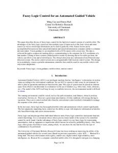
vehicle’s capacity). Also, we were able to prove that the underlying Markov chain has a special structure which facilitates decomposition of the Markov chain associated with the closedloop system into a finite number of Markov chains that have a smaller state space. The special structure makes the analysis easier and simplifies the computations considerably because it is easier to handle the smaller Markov chains associated with the subsystems. Furthermore, the model can be used for some distributions in the arrival of jobs at machines that satisfy a property that we identify. Depending on the nature of the system, the pick-up points could either be production machines (jobs) or offices (paperwork), and the dropoff point could be a conveyor belt or the main office. The work of Thonemann and Brandeau [24] is closest to our work in spirit because they also analyze a single vehicle in a closed loop path, but they primarily deal with a “dropoff” system, i.e., a system in which the AGV drops off material at each point and picks up material at a depot. The randomness in their system is in the arrival of jobs to the depot. They do not optimize the AGV’s capacity and consider only Poisson arrivals. We focus on a “pick-up AGV,” (found in local industries in Colorado) i.e., an AGV that picks up loads at various stations and drops them off at one point. The Markov chain approach enables us to compute some QoS measures, e.g., the probability of the AGV departing from a station leaving number of jobs stranded, and determine the optimal capacity of the AGV. To the best of our knowledge, this is the first attempt at both of these tasks in the literature. The rest of this paper is organized as follows. Section II describes the problem. Section III develops the Markov chain model. The performance measures and the optimization model are described in Section IV. Numerical results are presented in Section V. The last section presents some conclusions drawn from our work and some directions for further research in this topic. II. PROBLEM DESCRIPTION We first discuss some important features of the problem under consideration. The AGV travels in a fixed circuit from a dropoff point (e.g., conveyor belt) to each machine in a sequence (Machine 1, then Machine 2, and so on until all the machines have been visited) picking up jobs from each of the machines. The AGV then returns to the dropoff point to drop the jobs off and then repeats the circuit. The AGV takes a fixed (deterministic) amount of time to travel from one location to another; this time includes the unloading or loading time. The AGV empties itself completely at the dropoff point. Also, we assume that the route of the AGV is not influenced by whether it is full, although when it is full, it cannot pick up any more jobs in that trip. Jobs arrive at each location with random interarrival times that are independent and identically distributed; the amount of space (output buffer) near the pick-up point (machine) is fixed. In other words, when this buffer is full, the machine stops producing and thus the number of jobs waiting at each machine has an upper limit. Although the amount of space (buffer) at the machine is fixed, it is assumed that the buffer is of a sufficient size that the maximum number of jobs that can be waiting at the machine is rarely reached. Fig. 1 presents a schematic of the system.
506
IEEE TRANSACTIONS ON AUTOMATION SCIENCE AND ENGINEERING, VOL. 5, NO. 3, JULY 2008
In order to construct a discrete-time Markov chain, i.e., uniformize, we must discretize time. We let denote a positive and small unit of time. We then have the following definition. , let denote the max1) Definition 3.1: For imum length of the time interval during which the probability of two or more arrivals of jobs, at the th machine, is less than , i.e., (2) where is the number of arrivals at the th machine during a time interval of length . Next we introduce some notation. Maximum number of jobs that can wait at the th machine.
Fig. 1. Schematic view of n-machine system.
The performance metrics that we explore for evaluation and optimization of the system are: 1) average number of jobs waiting at each machine; 2) probability that the number of jobs waiting at a machine when the AGV departs from the same machine exceeds a given value; 3) average long-run cost of running the system.
Time spent by the AGV in traveling from machine to machine where machine 0 is the dropoff point. This also includes the loading time and the unloading time on machine when . when An integer multiple of
such that (3)
Probability that jobs arrive at the th machine in a time interval of length . Number of states in the th Markov chain. (States are defined below in Definition 3.2.)
III. MARKOV CHAIN MODEL A. System State
Maximum capacity of the AGV.
We introduce a Markov chain model for analyzing the system. Let the set denote the entire system that contains machines (or pick-up points). Then
Actual available capacity of the AGV. (It is a random variable for all machines but the first for which it equals .)
Dropoff point, Machine 1, Machine 2 A subset of
, called
denote the time between the th and the ( )th Let arrival of jobs at machine . Then, since jobs continually arrive at each machine, for any
Machine
, can be defined as follows: (1)
(4)
for . The behavior of the above-described system can be modeled with a sequence of Markov chains associated with the following:
, folWe will observe the system after unit time, i.e., lowing a standard convention in the literature (see [18, p. 435]), and after unit time, a new epoch will be assumed to have begun. , the length (time duration) of any Thus, if one specifies . epoch in the th Markov chain will equal The following phenomena will be treated as events for the th Markov chain: 1) A job arrives at a machine; 2) the AGV departs from the th machine; and 3) the AGV arrives at the th machine. An event will signal the beginning of a new epoch. The probability of two or more arrivals in one epoch will be assumed to be negligible for small , and the definition of ensures that. Furthermore, we will assume that if a job arrives during an epoch, we will move that event forward in time to is a small coincide with the end of that epoch. Since quantity, when is small, this should not pose serious problems. This approximation is necessary to ensure the Markov property
Dropoff point, Machine
The Markov chain associated with will be referred to as the th Markov chain. Because each machine will be analyzed independently, we consider Markov chains, one for each machine. Also, a nice property (Theorem 4.2) of the system is that one can use the invariant distribution (limiting probabilities) of th the th Markov chain to compute the same for the Markov chain. This provides for a simple recursive scheme that can be used to determine some important system performance measures associated with the entire system from the invariant distributions.
KAHRAMAN et al.: STOCHASTIC MODELING OF AN AUTOMATED GUIDED VEHICLE SYSTEM WITH ONE VEHICLE AND A CLOSED-LOOP PATH
for the system we consider. However, numerical results (presented later) will demonstrate that with the approximation we still have reasonably accurate results. Moreover, the approximation allows us to use the powerful framework of Markov chains. 2) Definition 3.2: Specify . A state of the th Markov chain in the th epoch is defined by the following 4-tuple: (5) denotes the number of jobs waiting at machine where when the th epoch begins, denotes the available capacity if the in the AGV when the th epoch begins, and AGV is traveling from the dropoff point to any machine while if the AGV is traveling from the th machine to the dropoff point when the th epoch begins. Since the th epoch could begin while the AGV is traveling either between the dropoff point and the machine or between the machine and denote the number of multiples of the dropoff point, we let that have elapsed until the beginning of the th epoch since the AGV’s departure. Clearly, the AGV’s departure could either be from the dropoff point or the th machine.
507
the probability of two or more arrivals converges to zero faster than either of the other two probabilities. In other words, for a small value of , one may practically ignore the event associated with more than two arrivals. With a small , we have for every a small enough , i.e., in the two properties above. Thus, with a sufficiently small duration of the epoch, one can safely ignore the probability of two or more arrivals for certain distributions. We will prove this when the interarrival time is exponentially distributed and uniformly distributed. Note, however, that even for these distributions, e.g., exponential, our approach remains approximate. 1) Theorem 3.1: If the interarrival time is exponentially dis, Properties 1 and 2 are satisfied. tributed with mean Proof:
thereby satisfying Property 1. Similarly
B. Transition Probabilities With the above discretization of time, we have the following property. For any small value of and for any , it is approximately true that by L'Hospital's rule
This implies that for nonzero, but small, , our system can be approximately modeled by a Markov chain. It is to be noted that the Markov chains constructed are essentially parametrized by the non-negative scalar . However, to keep the notation simple, and because is fixed, we will suppress this parameter. Thus, will be denoted by . By the definition, the th Markov chain is only concerned with job arrivals at the th machine. The definition of requires us to analyze whether the probability of two or more arrivals in an epoch can be ignored in comparison to that of zero or one arrival. We justify the use of a small with the following properties. Consider the following two properties assuming to be the duration of an epoch. Property 1:
(6)
2) Theorem 3.2: If the interarrival time is uniformly dis, Properties 1 and 2 are satisfied. tributed with Proof: For non-Poisson arrivals, to determine the probability distribution of the number of arrivals, one has to compute , the -fold convolution of the distribution of the interarrival time. If denotes the time of the th arrival (of job), then for the uniform distribution
Also
and
Then
Property 2:
(7) When the arrival distribution satisfies these two properties, one can ignore the probability of two or more arrivals in comparison to those of zero arrivals and one arrival as tends to zero because
Then, it follows that:
508
IEEE TRANSACTIONS ON AUTOMATION SCIENCE AND ENGINEERING, VOL. 5, NO. 3, JULY 2008
Property 1 is thus satisfied. Similarly, for Property 2, we have
by L'Hospital's rule
We show that the conditions (6) and (7) hold for the triangular distribution in Appendix I. For interarrival distributions (of jobs) that satisfy (6) and (7), we can develop expressions for the transition probabilities with a finite but small value of . The transitions are characterized by 12 conditions. For each Markov chain that we consider, we will assume, for the time being, that the available capacity is known. Subsequently, we will present a result (Theorem 4.2) to compute the distribution of . The state in the th epoch will be denoted by . The one-step transition probability will . be denoted by Fig. 2 presents a pictorial representation of the underlying Markov chain in our model. The available capacity of the AGV, , equals when it arrives at the first machine and is a random variable for all other machines. Then, , if , if (see 3.2), and . The transition probabilities for this Markov chain will now be defined for 12 conditions (cases). Cases 1–6 (7–12) are associated with the AGV traveling from the dropoff point to a machine (from a machine to the dropoff point). We now describe all the cases in detail. Consider the following scenario: the AGV travels from the dropoff point to machine during the th epoch, the arrival of the AGV at machine does not occur by the end of the epoch, and the buffer at machine is not full. Then, if no job arrives during the th epoch, we have the following. Case 1: If , , , , , , and , then Fig. 2. Markov chain underlying our model. B in figure stands for .
Since no job arrival occurs in “unit time,” the above transition probability is equal to the probability of no job arrival. Similarly, if a job arrival does occur, we have the following. Case 2: If , , , , , , and , then
Since job arrival occurs in “unit time,” the above transition probability is equal to the probability of job arrival. Consider the following scenario: the AGV travels from the dropoff point to the machine during the th epoch, the arrival of the AGV at machine does not occur by the end of the epoch and the buffer at machine is full. Then, we have the following.
Case 3: If , , and
,
,
,
, , then
Since the buffer at machine is full, we do not take job arrivals into consideration. Consider the following scenario: the AGV travels from the dropoff point to the machine during the th epoch, it arrives at machine by the end of the epoch, and the buffer at machine is not full. Then, if no job arrives during the current epoch, we have Case 4, and if a job arrives we have Case 5.
KAHRAMAN et al.: STOCHASTIC MODELING OF AN AUTOMATED GUIDED VEHICLE SYSTEM WITH ONE VEHICLE AND A CLOSED-LOOP PATH
Case 4: If ,
,
, ,
,
, and
,
Case 10: If , and
509
, ,
, ,
,
, then
then
Case 5: If ,
,
Case 11: If , , and
, , ,
, ,
, ,
, then
, and
, then
Consider the scenario in which the AGV travels from the dropoff point to machine during the th epoch, arrives at machine by the end of the th epoch, and the buffer at machine is full. Then, we have the following. , , Case 6: If , , , , and , then
Finally, consider the scenario in which the AGV travels from machine to the dropoff point during the th epoch, it arrives at the dropoff point by the end of the epoch, and the buffer at machine is full. Then, we have the following. , , Case 12: If , , , , and , then
IV. PERFORMANCE MEASURES AND OPTIMIZATION
Consider the scenario in which the AGV travels from machine to the dropoff point during the th epoch, the arrival to the dropoff point does not occur by the end of the epoch and the buffer at machine is not full. Then, if no job arrives during the th epoch, we have Case 7, and if a job does arrive we have Case 8. , , Case 7: If , , , , and , then
Case 8: If ,
, , , and
, ,
From Definition 3.2, the number of states in the th Markov , can be computed as chain, i.e.,
The following well-known result allows us to determine the invariant distribution (limiting probabilities) of the underlying Markov chains. 1) Theorem 4.1: Let denote the one-step transition probability matrix of a Markov chain. If the matrix is aperiodic and irreducible, and if , whose th element is denoted by , denotes a column vector of size , then solving the following system of linear equations yields the limiting probabilities of the Markov chain: and
, then
Consider the scenario in which the AGV travels from machine to the dropoff point during the th epoch, the arrival to the dropoff point does not occur by the end of the th epoch and the buffer at machine is full. Then, we have the following. Case 9: If , , , , , , and , then
Consider the scenario in which the AGV travels from machine to the dropoff point during the th epoch, it arrives at the dropoff point by the end of the epoch, and the buffer at machine is not full. Then, if no job arrives during the th epoch, we have Case 10. If a job arrival occurs during the th epoch, we have Case 11.
From the definition of our transition probabilities, it is not hard to show that each state is positive recurrent and aperiodic and that there is a single communicating class of states. Then, the above result holds and we may use it to compute the limiting probabilities. We next define a function, , that assigns an integer value in to each state in the th Markov chain the set
where denotes the state in the th Markov chain at a given epoch, . Note that , the epoch index, is suppressed here from the notation of (5) to increase clarity. Our transition probabilities for the th Markov chain were computed under the
510
IEEE TRANSACTIONS ON AUTOMATION SCIENCE AND ENGINEERING, VOL. 5, NO. 3, JULY 2008
Fig. 3. Computational scheme based on Theorem 4.2.
assumption that capacity of the AGV when it arrives at the th machine is known ( ). We now need to compute the transition probabilities of the entire system—the transition probabilities that we need for our performance evaluation model. We will provide a result, Theorem 4.2, to this end. The main idea underlying the result is as follows. The transition probabilities of the th Markov chain yield the distribution of the AGV’s available th Markov chain. Because the AGV starts capacity of the empty, for the first Markov chain, the available capacity is known to be . From that point onwards, one can compute the transition probabilities in a recursive style. The computational scheme based on the next result is depicted in a flowchart in Fig. 3. 2) Theorem 4.2: Let the limiting probability of state in the th Markov chain be denoted by . Let denote the available capacity of the AGV when it arrives at the th machine, and further let denote the limiting prob. ability for the state in the th Markov chain when Then, we have that (8) and
Proof: For the proof, we need to justify (8)–(10). Equation (8) follows from the fact that the AGV empties itself at the dropoff point (see Fig. 1). Hence, when it comes to Machine 1, the available capacity is not a random variable but a constant equal to , which is the maximum capacity of the AGV. Equation (9) follows from the fact that when the AGV arrives at stations numbered 2 through , its capacity is a random variable whose distribution has to be calculated. The distribution is given in (10). For the last statement, we argue as follows: When the , its caAGV arrives at the th station, for pacity is the available capacity of the AGV when it leaves the th station. The distribution for the available capacity on th station can be computed the AGV when it leaves the th from the limiting probabilities associated with the Markov chain of those states in which the AGV has departed th machine and is on the way to the th machine. the denotes the set of states in the th Markov (Note that th machine and chain in which the AGV has departed the its available capacity is . Similarly, denotes the set of states in the th Markov chain in which the AGV has departed th machine and its available capacity assumes from the all possible values.) Exploiting the transition probabilities, one can derive expressions for some useful performance measures of the system. They are considered next. denotes 3) Average Inventory at Each Machine: If the average number of jobs waiting at the th machine, then (11) where
and if if 4) QoS Performance Measure Associated With Downside Risk: The probability that the number of jobs waiting at the th machine, denoted by , when the AGV departs from the th machine exceeds can be calculated as follows:
(9) (12) for
,
, where where (10)
in which
and
and
are defined as follows:
5) Average Long-Run Cost: The average long-run cost of running the system is composed of two elements, which are: the holding cost of the jobs near the machine and the cost of operating the AGV. To calculate the holding cost, we will need the average number of jobs waiting at each machine. Then, the average cost for operating a system described in this paper, with
KAHRAMAN et al.: STOCHASTIC MODELING OF AN AUTOMATED GUIDED VEHICLE SYSTEM WITH ONE VEHICLE AND A CLOSED-LOOP PATH
machines to be served by an AGV whose capacity is given by
, is
(13) where and are constants representing the operating cost per unit time of an AGV having unit capacity and the holding cost per a unit time for one job, respectively; denotes the fixed cost of the vehicle In the uniformization procedure, the probability of two or more arrivals in one epoch is neglected. Thus, a few arrivals are unaccounted for. This causes a reduction in the values of both performance measures, i.e., and , for the first machine. This error affects the capacity distribution and results in a reduced available capacity for the AGV when it visits the subsequent machines. This error in the capacity distribution partly negates the error introduced by uniformization. Hence, at all machines but the first, where there is no error in estimating the capacity, the overall error in the performance-measure values is low. At the first machine, the capacity is equal to the maximum capacity, and so this reduction does not occur, thereby producing a higher error. This is reflected in the numerical results presented later. Also note that one has to find the limiting probabilities of different Markov chains, one chain associated with a specific machine in the system. However, to find the limiting probability of the specific state in a Markov chain associated with machine , where , one has to find the limiting probabilities different Markov chains associated with machine of the (see Theorem 4.2), since the available capacity of the AGV can assume any value between zero and when it arrives at any machine but the first machine. (Note that since the available capacity of the AGV is when it arrives at the first machine, the limiting probabilities of the Markov chain associated with the first machine can be found without the use of Theorem 4.2.) Hence, the computational work associated with any given machine but the first constitutes of the computational work of Markov chains calculating the limiting probabilities of plus the limiting probabilities of the Markov chain associated with the given machine via Theorem 4.2. Therefore, the complexity of the Markov chain model is a first-order polynomial in the number of machines . The advantage of our computational scheme is that the state space collapses for each Markov chain, thereby making the computation of the limiting probabilities feasible. 6) AGV Capacity Optimization: We are interested in optimizing the AGV’s capacity with respect to the cost of operating the system. The optimization problem considered in this paper to minimize the expression in (13). Other is to determine ways for optimization could be considered depending on what the manager desires. One example is to minimize
such that
where and are set by managerial policy. Optimization is performed by an exhaustive enumeration of the AGV’s maximum capacity variable, . Since the state
511
space of this discrete optimization problem, which has a single decision variable, is very small, an exhaustive enumeration is feasible. V. COMPUTATIONAL RESULTS Simulation is by far the most extensively used tool for performance evaluation of AGV systems, because it provides us with very accurate estimates of performance measures. As a result, it is essential that we compare our results to those obtained from a simulation model. A. Simulation Model Consider a probability space , where denotes the (universal) set of all possible round trips of the AGV, denotes the sigma field of subsets of , and denotes a probability mea. Using a discrete-event simulator, it is possible sure on from the measurto generate random samples able space. The samples can then be used to estimate values of all the performance measures derived in the previous section. denote the number of jobs waiting near the th Let machine at time in the simulation sample . Then, from the strong law of large numbers, with probability 1 (14) Also, with probability 1 (15) where denotes the number of occasions in which the number of jobs left behind at machine (i.e., jobs not picked up by the AGV because it is full) equals or exceeds in visits to the machine in the simulation sample . B. Performance Tests for Markov Model We conducted numerical experiments with our model to determine the practicality of the approach and to benchmark its performance with a simulation model that is guaranteed to perform well but is considerably slower. The error of our model with respect to the simulation estimate is defined by Error (%) where denotes the estimate from the Markov chain model and denotes the same from the simulation model. We present results on two-machine and five-machine systems, along with a simple example to illustrate our methodology. Tables I and II define the parameters for the systems with two machines, and Tables XI and XII define the parameters defor the systems with five machines studied. In Table I, notes the rate of arrival of jobs at machine . We used the exponential and gamma to model the distribution of the interarrival time of jobs. The performance metrics of the systems with two machines and five machines are shown in Tables III–VIII and Tables XIII–XX, respectively. These tables also show the simulation estimates and the corresponding error values which are calculated as defined above. Convergence was achieved with
512
IEEE TRANSACTIONS ON AUTOMATION SCIENCE AND ENGINEERING, VOL. 5, NO. 3, JULY 2008
TABLE I SYSTEM (SYS.) PARAMETERS. VALUE OF IS 0.05 FOR EACH SYSTEM AND EACH SYSTEM HAS TWO MACHINES
TABLE IV AVERAGE NUMBER OF JOBS WAITING AT MACHINE 2 FOR POISSON ARRIVALS
TABLE II SYSTEM (SYS.) PARAMETERS (CONTINUED) TABLE V AVERAGE NUMBER OF JOBS WAITING AT MACHINE 1 FOR GAMMA-DISTRIBUTED INTERARRIVAL TIME
TABLE III AVERAGE NUMBER OF JOBS WAITING AT MACHINE 1 FOR POISSON ARRIVALS
1000 trips per replication and we used ten replications. The mean estimate was assumed to have converged when it remained within 0.05% in the next iteration. The mean reported is an average over all replications. The standard deviation was no more than 0.1% of the mean in each case. 1) 2-Machine Systems: Tables III and IV provide for Poisson arrivals for and , respectively. Similarly, Tables V and VI show the corresponding values for a gamma-distributed interarrival time. In these systems, i.e., in the systems with two machines, for the gamma distribution we used the same arrival rate, but the parameter was set to eight. Tables VII and VIII show the values of with and , respectively; Tables IX Poisson arrivals for and X show the corresponding values for a gamma-distributed interarrival time.
KAHRAMAN et al.: STOCHASTIC MODELING OF AN AUTOMATED GUIDED VEHICLE SYSTEM WITH ONE VEHICLE AND A CLOSED-LOOP PATH
TABLE VI AVERAGE NUMBER OF JOBS WAITING AT MACHINE 2 FOR GAMMA-DISTRIBUTED INTERARRIVAL TIME
TABLE VIII PROBABILITY THAT AGV LEAVES TWO OR MORE JOBS BEHIND FOR POISSON ARRIVALS
TABLE VII PROBABILITY THAT AGV LEAVES TWO OR MORE JOBS BEHIND FOR POISSON ARRIVALS
2) Example: Consider System 5, whose parameters are given in Tables I and II. In this system, jobs arrive at the rate of 2 . Here, per unit time at each machine. We choose for . The AGV travels from the dropoff point to Machine 1, from Machine 1 to Machine 2, and from Machine 2 to the dropoff point in time equaling , , and , respectively. The maximum capacity of the AGV is 2, and the buffer capacities of each machine are 4. We provide some sample transition probabilities for the Markov chain associated with Machine 1 Case 1: Case 3: Case 5: Case 10:
513
TABLE IX PROBABILITY THAT AGV LEAVES TWO OR MORE JOBS BEHIND FOR GAMMA-DISTRIBUTED INTERARRIVAL TIME
The capacity of the AGV when it arrives at machine 1 is , and the capacity distribution of the AGV when it arrives at Machine 2 is calculated using Theorem 4.2
and
Then, the transition probabilities for the second Markov chain can be calculated from the distribution of . The limiting probabilities can then be used to calculate the values of the performance measures, such as the average inventory and the downside risk.
514
IEEE TRANSACTIONS ON AUTOMATION SCIENCE AND ENGINEERING, VOL. 5, NO. 3, JULY 2008
TABLE X PROBABILITY THAT AGV LEAVES TWO OR MORE JOBS BEHIND FOR GAMMA-DISTRIBUTED INTERARRIVAL TIME
TABLE XIII AVERAGE NUMBER OF JOBS WAITING AT EACH MACHINE FOR POISSON ARRIVALS
TABLE XIV TABLE XIII (CONTINUED) AVERAGE NUMBER OF JOBS WAITING AT EACH MACHINE FOR POISSON ARRIVALS
TABLE XI SYSTEM (SYS.) PARAMETERS. VALUE OF IS 0.05 FOR EACH SYSTEM, INTERARRIVAL TIMES ARE i. i. d., EXPONENTIALLY DISTRIBUTED AND EACH SYSTEM HAS FIVE MACHINES
TABLE XV AVERAGE NUMBER OF JOBS WAITING AT EACH MACHINE FOR GAMMA DISTRIBUTED INTERARRIVAL TIMES TABLE XII SYSTEM (SYS.) PARAMETERS. VALUE OF IS 0.05 FOR EACH SYSTEM, INTERARRIVAL TIMES ARE i. i. d., GAMMA DISTRIBUTED AND EACH SYSTEM HAS FIVE MACHINES. G DENOTES GAMMA
3) Five-Machine Systems: Tables XIII and XIV list the for , and Tables XVII and values of XVIII list the values of for for
Poisson arrivals. The corresponding values for a gamma-distributed interarrival time are shown in Tables XV and XVI (for the average number waiting) and Tables XIX and XX (for the probability). Tables XXI and XXII present the results from optimization performed with the Markov chain model. Fig. 4
KAHRAMAN et al.: STOCHASTIC MODELING OF AN AUTOMATED GUIDED VEHICLE SYSTEM WITH ONE VEHICLE AND A CLOSED-LOOP PATH
515
TABLE XVI TABLE XV (CONTINUED) AVERAGE NUMBER OF JOBS WAITING AT EACH MACHINE FOR GAMMA DISTRIBUTED INTERARRIVAL
TABLE XIX PROBABILITY THAT AGV LEAVES TWO OR MORE JOBS BEHIND FOR GAMMA DISTRIBUTED INTERARRIVAL TIMES
TABLE XVII PROBABILITY THAT AGV LEAVES TWO OR MORE JOBS BEHIND FOR POISSON ARRIVALS
TABLE XX TABLE XX (CONTINUED). PROBABILITY THAT AGV LEAVES TWO OR MORE JOBS BEHIND FOR GAMMA DISTRIBUTED INTERARRIVAL TIMES
TABLE XVIII TABLE XVII (CONTINUED) PROBABILITY THAT AGV LEAVES TWO OR MORE JOBS BEHIND FOR POISSON ARRIVALS
TABLE XXI OPTIMIZED CAPACITY (Z ) AND OPTIMAL COST (C ) FOR SYSTEMS WITH TWO MACHINES. HERE, c = $300, c = $550, AND c = $10000
TABLE XXII OPTIMIZED CAPACITY (Z ) AND OPTIMAL COST (C ) FOR SYSTEMS WITH FIVE MACHINES. HERE, c = $300, c = $550, AND c = $10000
shows the cost values for the different capacities and the need for optimization. Figs. 5 and 6 show the effect of a bigger value of on the for Systems 30 and 31, respectively. Figs. 7 value of for Systems and 8 show the effect of the same on 30 and 31, respectively. As seen from these graphs, the accuracy of the Markov model decreases as increases. Clearly, as decreases, the discrete-time approximation gets closer to its continuous limit [see (2) and (4)].
The major conclusion from our experiments is that the Markov chain model produces a solution with a good quality and does so in a very reasonable amount of computer time, which is less than 2 minutes on a Pentium processor PC with 2-GHz CPU frequency and 250-MG RAM size. The simulation model in comparison takes about four times as much time.
516
IEEE TRANSACTIONS ON AUTOMATION SCIENCE AND ENGINEERING, VOL. 5, NO. 3, JULY 2008
Fig. 4. Total cost versus capacity of AGV for System 2.
1 P [D(n) > 1] in System 30. Errors in other P [D(1) > 1] P [D(2) > 1], and P [D(5) > 1] are even 1
Fig. 7. Effect of a bigger on parameters, i.e., , smaller for plotted values of .
Fig. 5. Effect of a bigger and eters, i.e.,
[W (4)]
1 on [W (n)] in system 30. Errors in other param[W (5)] are even smaller for plotted values of 1. 1 P [D(n) > 1] in System 31. Errors in other P [D(1) > 1] P [D(2) > 1], P [D(4) > 1], and P [D(5) > 1.
Fig. 8. Effect of a bigger on parameters, i.e., , are even smaller for plotted values of
1]
VI. CONCLUSION
Fig. 6. Effect of a bigger eters, i.e., and
[W (4)]
1 on [W (n)] in System 31. Errors in other param[W (5)] are even smaller for plotted values of 1.
The simulation model and the theoretical model make identical assumptions about the system. The computer codes can be requested from the first author.
In this paper, we studied a version of a problem commonly found in small-scale manufacturing industries, e.g., pharmaceutical firms, which require no more than one AGV that operates in a closed-loop path. We used a Markov chain approach for developing the performance-analysis model. Some special properties of the system were exploited to define a simple structure to the complete problem; the structure allows us to decompose the -machine system (Markov chain) into individual systems (Markov chains) and provides us with a mechanism to simplify the computations. This leads to a state-space collapse that is computationally enjoyable. Also, the discretization of the state space in our approach yielded simple expressions for the transition probabilities; a common criticism of many transition-probability models is that they have complicated expressions with multiple integrals (that require numerical integration, which is slow) as transition probabilities.
KAHRAMAN et al.: STOCHASTIC MODELING OF AN AUTOMATED GUIDED VEHICLE SYSTEM WITH ONE VEHICLE AND A CLOSED-LOOP PATH
Some of the advantages of the Markov chain approach are as follows: 1) It is easy to understand; the transition probabilities are characterized by 12 simple conditions. 2) It is simple conceptually because all one needs is (where denotes the cdf of the job interarrival time), which can be easily calculated for any distribution for the interarrival time of jobs. 3) It produces a state-space collapse thereby making it feasible to compute the limiting probabilities. And finally, 4) it is quite accurate; this is reflected by favorable comparisons with a simulation benchmark. The main theme of this paper was to develop a simple, although approximate, Markov chain to help study the performance of an AGV system (with one vehicle and a closed-loop path) and optimize its capacity. The cost and capacity of the AGV are two parameters that are inextricably linked to each other, and this was an attempt to quantify and analyze this relationship. Extending this model to “dropoff” AGVs, multiple AGVs, or systems that do not share some of the properties assumed here should make for exciting topics for further research. APPENDIX Theorem A.1: If the interarrival time is triangularly distributed with , Properties 1 and 2 are satisfied. Proof: For the triangular distribution, for
Also, for
and
Since we are interested in obtaining the limits for zero, we do not consider the case for . Then
tending to
Then, it follows that
Property 1 is thus satisfied. Similarly, for property 2, we have
applying L'Hospital's rule twice
517
ACKNOWLEDGMENT The authors would like to thank all the reviewers for their detailed comments; in particular, they express gratitude to the reviewer who suggested a new title for the paper and made several other comments that were used to improve the quality of this work. REFERENCES [1] O. Bakkalbasi, “Flow path network design and layout configuration for material delivery systems,” Ph.D. dissertation, Georgia Inst. Technology, Atlanta, GA, 1989. [2] Y. A. Bozer and J. H. Park, “New partitioning schemes for tandem AGV systems,” in Progress in Material-Handling Research, 1992. Ann Arbor, MI: Braun-Brunfiled, 1993, pp. 317–332. [3] Y. A. Bozer and M. M. Srinivasan, “Tandem AGV systems: A partitioning algorithm and performance comparison with conventional AGV systems,” Eur. J. Operational Res., vol. 63, pp. 173–191, 1992. [4] P. Chevalier, Y. Pochet, and L. Talbott, “Design of a 2-stations automated guided vehicle systems,” in Quantitative Approaches to Distribution Logistics and Supply Chain Management, A. Kolse, M. Speranza, and L. W. Eds, Eds. Berlin, Germany: Springer, 2002, pp. 309–329. [5] J. Duan and J. Simonato, “American option pricing under GARCH by a Markov chain approximation,” J. Economic Dynamics Contr., vol. 25, no. 11, pp. 1689–1718, 2001. [6] P. J. Egbelu, “The use of non-simulation approaches in estimating vehicle requirements in an automated guided vehicle based transport system,” Mater. Flow, vol. 4, pp. 17–32, 1987. [7] P. J. Egbelu and J. M. A. Tanchoco, “Characterization of automatic guided vehicle dispatching rules,” Int. J. Production Res., vol. 22, no. 3, pp. 359–374, 1984. [8] Gendreau and M. Etude, “Approfondi d’un modele d’equilibre pour l’affectation des passagers dans les reseaux de transport en commun,” Ph.D. dissertation, Univ. de Montreal, Montreal, Canada, 1984. [9] S. Heragu, Facilities Design. Boston, MA: PWS, 1997. [10] M. E. Johnson and M. L. Brandeau, “Stochastic modeling for automated material handling system design and control,” Transportation Sci., vol. 30, no. 4, pp. 330–348, 1996. [11] P. Koo, J. Jang, and J. Suh, “Estimation of part waiting time and fleet sizing in AGV systems,” Int. J. Flexible Manuf. Syst., vol. 16, pp. 211–228, 2005. [12] H. J. Kushner and P. Dupuis, Numerical Methods for Stochastic Control Problems in Continuous Time, 2nd ed. New York: Springer, 2001. [13] A. M. Law and W. D. Kelton, Simulation Modeling and Analysis. New York: McGraw-Hill, 2000. [14] L. Leung, S. K. Khator, and D. Kimbler, “Assignment of AGVs with different vehicle types,” Mater. Flow, vol. 4, no. 1–2, pp. 65–72, 1987. [15] B. Mahadevan and T. T. Narendran, “Estimation of number of AGVs for FMS: An analytical model,” Int. J. Production Res., vol. 31, no. 7, pp. 1655–1670, 1993. [16] W. L. Maxwell and J. A. Muckstadt, “Design of automated guided vehicle systems,” IIE Trans., vol. 14, no. 2, pp. 114–124, 1982. [17] W. B. Powell, “Iterative algorithms for bulk arrival, bulk service, and non-Poisson arrivals,” Transportation Sci., vol. 20, pp. 65–79, 1986. [18] S. M. Ross, Introduction to Probability Models. San Diego, CA: Academic, 1997. [19] J. J. Solberg, “A mathematical model of computerized manufacturing systems,” in Proc. 5th Int. Conf. Production Res., Tokyo, Japan, Aug. 1977. [20] M. M. Srinivasan, Y. A. Bozer, and M. Cho, “Trip-based handling systems: Throughput capacity analysis,” IIE Trans., vol. 26, no. 1, pp. 70–89, 1994. [21] Subramaniam, J. S. Stidham, Jr, and C. J. Lautenbacher, “Airline yield management with overbooking, cancellations and no-shows,” Transportation Sci., vol. 33, no. 2, pp. 147–167, 1999. [22] J. M. A. Tanchoco, P. J. Egbelu, and F. Taghaboni, “Determination of the total number of vehicles in an AGV-based material transport system,” Mater. Flow, vol. 4, no. 1–2, pp. 33–51, 1987. [23] T. Tansupawuth, “Optimizing the capacity of an AGV using a stochastic simulation,” M.S. thesis, Colorado State Univ., Pueblo, 2002. [24] T. U. M. I. Wrandeau, “Designing a single-vehicle automated guided vehicle system with multiple load capacity,” Transportation Sci., vol. 30, no. 4, pp. 351–353, 1996.
518
IEEE TRANSACTIONS ON AUTOMATION SCIENCE AND ENGINEERING, VOL. 5, NO. 3, JULY 2008
[25] J. A. Tompkins, J. A. White, Y. A. Bozer, E. H. Frazelle, J. M. A. Tanchoco, and Trevino, Facilities Planning. New York: Wiley, 1995. [26] I. Vis, R. de Coster, K. Roodbergen, and L. Peeters, “Determination of the number of AGVs required at a semi-automated container terminal,” J. Operational Res. Soc., vol. 52, no. 4, pp. 409–417, 2001. [27] R. A. Wysk, P. J. Egbelu, C. Zhou, and B. K. Ghosh, “Use of spread sheet analysis for evaluating AGV systems,” Mater. Flow, vol. 4, pp. 53–64, 1987.
Aykut F. Kahraman received the B.S. degree from the Electrical and Electronics Engineering Department, Bilkent University, in 2002, the M.S. degree from the Industrial and Systems Engineering Department, Colorado State University, Pueblo, in 2003, and the Ph.D. degree from the Industrial and Systems Engineering Department, State University of New York, Buffalo, in 2006. His research interests include logistics, service and manufacturing systems, and performance evaluation in stochastic systems. Application domains that interest him are primarily in the aviation industry and the manufacturing industry. In the field of stochastic optimization, he has specialized in the area of discrete-time Markov chains, Markov decision processes, semi-Markov decision processes, and stochastic dynamic programming. Currently, he is working as an Operations Research Developer at Deccan International, San Diego, CA.
Abhijit Gosavi (M’06) received the B.S. degree from Jadavpur University, the M.S. degree from the Indian Institute of Technology, Madras, and the Ph.D. degree in industrial engineering from the University of South Florida, in 1999. He is currently an Assistant Professor in the Department of Industrial and Systems Engineering, State University of New York, Buffalo. His research interests include the applications and methods of control theory and simulation-based optimization. His publications have appeared in leading journals like Management Science, Automatica, and Machine Learning.
Karla J. Oty received the B.S. degree in mathematics from Trinity University, San Antonio, TX, and the Ph.D. degree from the University of Colorado, Boulder, under the direction of Prof. A. Ramsay. Her dissertation in analysis was entitled “Fourier-Stieltjes Algebras for R-discrete Groupoids.” Having taught for 13 years at schools in Oklahoma and Colorado, she is currently serving as Interim Dean of the School of Science and Technology, Cameron University, Lawton, OK. Dr. Oty has received various awards including Cameron University’s “Professor of the Year” for the academic year 2005–2006.