system state process imposing a bound on the average over time of state constraint ...... In 2012 IEEE 51st IEEE Conference on Decision and. Control (CDC) ...
Stochastic MPC for Controlling the Average Constraint Violation of Periodic Linear Systems with Additive Disturbances Luca Fabietti and Colin N. Jones Abstract— This paper deals with stochastic model predictive control of constrained discrete-time periodic linear systems. Control inputs are subject to periodically time-varying polytopic constraints with possibly time-dependent state and input dimensions. A stochastic constraint is instead enforced on the system state process imposing a bound on the average over time of state constraint violations. Disturbances are additive, bounded and described by a periodically time-dependent probabilistic distribution. The aim of this paper is to develop a receding horizon control scheme which enforces recursive feasibility for the closed-loop state process. The effectiveness of the proposed algorithm is finally shown through a simulation study on a building climate control case.
I. INTRODUCTION In recent years, many MPC algorithms to robustly control systems subject to external disturbances and model uncertainties have been developed. A standard approach is to consider the perturbation to have a bounded support and, exploiting this information, to guarantee desired results such as stability and recursive feasibility, e.g [1], [2]. However, these methods completely disregard any a-priori known stochastic information on the disturbance which is often available from the structure of the problem or from historical data. Therefore, relying on a worst-case approach, the performance of the resulting controller is often highly conservative preventing the extensive use of these algorithms in practical applications. To fill the gap between sound theoretical results and real life applications, Stochastic MPC (SMPC) has emerged as a new area of research. This is due to the fact that this control scheme is designed to directly account for the stochastic nature of the disturbance and it is therefore capable of reducing the conservatism of its robust counterpart. Moreover, in many practical problems, constraint specification is, by nature, probabilistic so that it is reasonable to allow violations to occur with a certain frequency or when the amount by which the constraint is violated is small. The main challenge within this framework is recursive feasibility. Standard methods consider point-wise in time constraint specifications such as expectational, probabilistic or integrated chance constraints. These constraints are then The authors are with the Automatic Control Laboratory in EPFL, Lausanne, Switzerland. {luca.fabietti, colin.jones}
@epfl.ch This work has received support from the Swiss National Science Foundation under the NRP 70 Energy Turnaround Project (Integration of Intermittent Widespread Energy Sources in Distribution Networks: Storage and Demand Response, grant number 407040 15040/1) and the European Research Council under the European Unions Seventh Framework Programme (FP/2007-2013) / ERC Grant Agreement n. 307608 (BuildNet)
typically enforced by implementing a mixed stochasticworst-case tightening procedure [3], [4]. However, these approaches do not consider past trajectories of the state process and this generally results in a conservative formulation. A different approach was first proposed in [5] and then extended in [6]. The main idea is to reduce the conservatism of previous methods by looking at the whole history of the state trajectory. Hence, rather than controlling the amount of constraint violations at each time separately, the quantity of interest is the average over time of constraints violations. All the aforementioned approaches focused on LTI systems subject to time-invariant disturbances which is a quite restrictive assumption in many applications. Periodic linear systems offer a useful generalization of time-invariant systems providing a natural framework for modeling various phenomena [7]. A relevant example of this is represented by building climate control where the system is subject to timevarying environmental perturbations that typically present periodic, seasonal/daily patterns. MPC of linear/nonlinear periodic systems has been tackled in many contributions [8]– [10]. The case of linear periodic systems subject to additive uncertainties has been considered, yet in a robust setting, in [11]. To the best of authors’ knowledge the control of a periodic linear system in an SMPC framework has not been addressed, which was one of the main motivations for this paper. The contribution, and novelty, of this manuscript is twofold. First we generalize the concepts of periodic controlled invariant sets, available in the robust framework [11], to the stochastic case. Second we provide the extension of the least-conservative approach of [6] to the powerful and more general class of discrete-time periodic linear systems with periodically time-varying system dimensions and subject to additive time-varying disturbances. Notation Throughout the article, Rn denotes the ndimensional real space, uppercase letters are used for matrices and lower case for vectors. ak represents the value of vector a at time k. N+ stands for the set of non-negative integers whereas Nkj is the set of non-negative integers {j, . . . , k}. Random variables are defined on a common probability space where a probability measure, P (·), is also defined; the expectation E{·} is taken with respect to this measure. The symbol I[x > 0] is used to denote the indicator function of the event [x > 0].
II. P ROBLEM S TATEMENT Definition 1: A discrete time linear periodic system is defined by: xk+1 = Aσk xk + Bσk uk + wk σk := mod(k, p) σk : N → N0p−1
(1)
with system time step k ∈ N, period length p ∈ N+ , intraperiod step index function σ(·), state xk ∈ Rnσk , input uk ∈ Rmσk , disturbance wk ∈ Rlσk and Aσk ∈ Rnσk+1 ×nσk , Bσk ∈ Rnσk+1 ×mσk . Remark 1: The dimensions of state, input and disturbance vectors are allowed to be periodically time-dependent and have to satisfy nj , mj , lj ∈ N+ ∀j ∈ Np−1 . The possibility to 0 consider systems characterized by time-varying dimensions can be useful in many practical situations, e.g., to model systems with asynchronous control inputs [11]. Another evidence of this fact is reported in Section IV-B. We assume that the state of the system is perfectly known at time k. The inputs are subject to hard constraints of the form: uk ∈ Uσk , k ∈ N+ (2) At each time step k, we assume the support of wk to belong to a compact polyhedron Wσk . Finally the closed-loop state of the process is required to satisfy, in a probabilistic fashion, the following constraint: gσTk xk ≤ hσk
(3)
nσk
where gσk ∈ R and hσk ∈ R. In order to quantify the amount of violations occurring at time k we introduce the concept of a loss function. Definition 2: A function l : R → R is a loss function if it is non-decreasing and lower-semicontinuos and it is zero at the origin. In loose terms, one wants the state to remain in the half space defined by (3) “most of the time” or alternately not to exceed it “very much”. Note that the state constraint can be time-varying as well. A possible way to formalize this requirement is to impose point-wise in time constraints such as E{l(gσTk xk
− hσk )} ≤ ξ,
k ∈ N+
(4)
where ξ ∈ [0, 1). In general, due to the fact that constraints of this type are hard to deal with, one wants to enforce (4) by means of the one-step conditional constraint. E{l(gσTk+1 xk+1 − hσk+1 )|xk )} ≤ ξ,
k ∈ N+
(5)
However, constraint (5) is, in general, very conservative which reduces the potential benefit of the probabilistic constraint specification. Instead of focusing on point-wise in time probabilistic constraints such as (4), we enforce constraints directly on the closed loop state process as a whole. To this aim, we first introduce the weighted cumulative loss up to time k vk :=
k X i=0
γ k−i l(gσTi xi − hσi ) k ∈ N+
(6)
where γ ∈ [0, 1] determines the forgetting rate of past losses. Secondly, we define the normalization factor sk ( k 1−γ k+1 X γ ∈ [0, 1) k−i 1−γ (7) sk := γ = k+1 γ=1 i=0 Hence, the ratio vk /sk represents the weighted average loss up to time k and it is the main quantity of interest of this manuscript. In particular we require that: vk vk+1 }≤ξ if ≤ξ (8a) Ek { s sk k+1 vk lim vmin(k+i,τk ) ≤ ξ if >ξ (8b) i7→∞ s sk min(k+i,τk ) where the integer number τk is the first time of return. More precisely, if at time k the amount of violations exceed the maximum allowed value, i.e. vk > ξsk , τk represents the first time after k when the condition vτk ≤ ξsτk is satisfied again, that is: τk := inf{i ≥ k | vi /si ≤ ξ} ∈ {k, k + 1, . . .}
(9)
III. M AIN R ESULT In this section a recursively feasible receding horizon control policy that enforces the constraint (8) for the closedloop state process is presented. The main idea is to apply feedback on the ratio vk /sk acting on the one-step conditional constraint (5). If the quantity vk /k is “small” we will loosen it, on the other hand, if it is “large” we will enforce (5) as it is. As a first step, it can be observed that, by exploiting the state dynamic (1), the conditional constraint (5) can be written as E{l(gσTk+1 (Aσk xk + Bσk uk + wk ) − hσk+1 )} ≤ ξ
(10)
The evaluation of (10) is in general difficult, hence to obtain a sufficient condition for its satisfaction, we first observe that the constraint (10) can be arranged as E{l(gσTk+1 (Aσk xk + Bσk uk ) − hσk+1 +gσTk+1 wk )} ≤ ξ {z } | µ
now, considering the function fσk (µ) := E{l(µ + gσTk+1 wk )}
(11)
one immediately recognizes that it can be written as Z ∞ fσk (µ) := l(µ + y)pdfgσT wk (y)dy −∞
k+1
Finally, the inequality (5) is satisfied if and only if gσTk+1 (Aσk xk + Bσk uk ) ≤ qσk (ξ) + hσk+1
(12)
where q : R → R is defined as qσk (ξ) := sup{µ ∈ R | fσk (µ) ≤ ξ} and its existence is guaranteed by the assumptions on the loss function l(·). In the following we will introduce key concepts that are useful for the understanding of the proposed algorithm.
Definition 3: The stochastic feasibility set Xjs corresponding to the intra-period index j = 0, . . . , p − 1 is defined as Xjs = {x ∈ Rnj : ∃u ∈ Uj | gσTj+1 (Aj x + Bj u) ≤ qj (ξ) + hσj+1 }
(13)
Essentially, Xjs represents the set of all states from which there exists an admissible input for the intra-period index j such that the state process will satisfy the constraint (5) for all the possible disturbance realizations contained in the current disturbance support set Wj . In many practical situations, besides the stochastic constraint (8), it is desirable that the amount of violations is constrained by a maximum admissible loss at each time iteration. l(gσTk x − hσk ) ≤ ξ¯σk (14) Typically the parameter ξ¯σk is derived from the problem specification and can be, in general, time-varying as well. This requirement defines the feasible set X¯j for each j = 0, . . . p − 1 X¯j := {x ∈ Rnj | gσTj x ≤ hσj + l−1 (ξ¯σj )}
(15)
where l−1 (a) := sup{y ∈ R|l(y) ≤ ξ} ∈ [−∞, ∞]
∧
∃u ∈ Uj : Aj x + Bj u + w ∈ Sσj+1 gσTj+1 (Aj x
∀w ∈ Wj
+ Bj u) ≤ qj (ξ) + hσj+1
(16) In the following, the parameter that will adjust the loosening of the one-step conditional constraint (5) is presented. Starting from the first line of (8) one can observe that the expected value Ek {vk+1 } can be written as Ek {vk+1 } = γvk + Ek {l(gσTk+1 xk+1 − hσk+1 )}
(17)
(20)
Remark 2: Please note that when βk > ξ, enforcing (20), guarantees the satisfaction of the first line of (8). On the contrary, this is not guaranteed whenever βk = ξ. Despite this, it is still possible to define a control policy which achieves to enforce satisfaction of (8). To this aim, we introduce an auxiliary state that controls the definition of the parameter β χk = ξsk − vk
(21)
For each k ∈ N+ , we further define the set U˜σk (xk , χk ) := {u ∈ Uσk : Aσk xk + Bσk u + w ∈ Sσk+1 ∀w ∈ Wσk E{l(gσTk+1 (Aσk xk
(22a)
+ Bσk u + wσk ) − hσk+1 )} ≤ βk } (22b)
A basic single-layer set-valued control policy that will lead to the satisfaction of (8) as a whole is then defined as k ∈ N+
(23)
The proof of this statement is given in the following section where a multi-layer version of the control policy is presented. A. Multi-layer version As already underlined, enforcing (8) is, in general, less conservative with respect to standard point-wise probabilistic constraints such as (5). Still the invariance constraint (22a) is independent of the amount of past violations, therefore it reduces the potential benefits of loosening the constraint (22b). Hence, in the following, we will relax the condition (22a) allowing the state process to move within a sequence of nested sets built around the SPCI sequence whenever the number of past violations is “small” enough. More precisely let’s first observe that, at time k and when xk+1 ∈ X¯σk+1 sk+1 ξ − vk+1 = sk+1 ξ − γvk − l(gσTk+1 xk+1 − hσk+1 )
The right side of the inequality (8), in turn ξsk+1 = ξ(γsk + 1) Therefore (8a) will be satisfied at time k if the following condition holds Ek {l(gσTk+1 xk+1 − hσk+1 )} ≤ γ(ξsk − vk ) + ξ
E{l(gσTk+1 xk+1 − hσk+1 )|xk } ≤ βk
κ ˜ σk (xk , χk ) ∈ U˜σk (xk , χk ),
The second important concept that needs to be introduced is that of Stochastic Periodic Controlled Invariance sequence (SPCI). Definition 4: A collection of sets (S0 , S1 , . . . , Sp−1 ), is an SPCI sequence if it satisfies for each j = 0, 1 . . . , p − 1 Sj ⊆ Xjs ∩ X¯j and ∀x ∈ Sj
Essentially, we will exploit βk to define a control policy which enforces the satisfaction of (8) as a whole. To this effect, at each time iteration, depending on the amount of previous constraint violations, we will enforce the constraint
(18)
Definition 5: The probability leeway βk ∈ [ξ, ∞) at time k ∈ N is βk := min{γ(ξsk − vk ) + ξ, ξ}1 (19) 1 Please note that the probabilistic leeway parameter β could be equivk alently � defined as ξ if ξsk < vk βk := γ(ξsk − vk ) + ξ if ξsk ≥ vk
= γ(sk ξ − vk ) + ξ − l(gσTk+1 xk+1 − hσk+1 ) ≥ γ(sk ξ − vk ) + ξ − ξ¯σ k+1
Continuing, we obtain sk+2 ξ − vk+2 = sk+2 ξ − γvk+1 − l(gσTk+2 xk+2 − hσk+2 ) = ξ(sk+1 γ − vk+1 ) + ξ − l(gσTk+2 xk+2 − hσk+2 ) ≥ γ 2 (sk ξ − vk ) + γ(ξ − ξ¯σ ) + ξ − ξ¯σ k+1
k+2
the same argument can be used to obtain a condition i steps ahead sk+i ξ−vk+i ≥ γ i (sk ξ − vk ) −
i X t=1
γ i−t (ξ¯σk+t − ξ)
Consequently, if xk+t ∈ X¯σk+t for each t ∈ {1, . . . , i}, the requirement sk+i ξ − vk+i is satisfied if (sk ξ − vk ) ≥
i X
γ
−t
(ξ¯σk+t − ξ)
(24)
t=1
In particular, if at time k, condition (24) is met, we are guaranteed that vk+i ≤ (k + i)ξ is satisfied without the imposition of any constraints besides xk+i ∈ X¯σk+i . This opens the possibility of letting the system state temporarily leave the SPCI sequence but still making sure that it will return at time k + i. To this end we define the concept of preset Pre(Mj ) =: {x ∈Rnj : ∃u ∈ Uj−1 | Aj x + Bj u + w ∈ Mj
∀w ∈ Wj } (25) The sequence of nested family of length ns is then obtained through Sj1 := Sj , k Sjk+1 := Pre(Sj−1 ),
∀j = 0, 1, . . . , p − 1
(26a)
∀j = 0, 1, . . . , p − 1
(26b)
∀k = 2, . . . , ns − 1 Now let’s assume the current time to be k and the state of the system to belong to the set Sσk . If condition (24) holds then the state is free to move up to the set Sσi+1 from which k+1 we are guaranteed to get back to Sσ1k+i+1 at time k + i + 1 where it might be necessary to enforce (22b). According to this argument, it is possible to introduce an index rt ∈ Nn1 s that determines to which layer the state is allowed to move. Define r˜k as S01
r0 = 1
S02
S11
S12
r1
S21
=
S01
S11
S21
2 S22
r2 = 2
S02
r3
S12
=
S22
= r4
3
S03
S13
S23
S03
S13
v0 = 0, r0 = 1
v1 = 0, r1 = 2
v2 = 0, r2 = 2
v3 = 0, r3 = 3
v4 = 1, r4 = 2
2 S23
Fig. 1. Possible evolutions of the state over several time steps when starting from set S01 at time k = 0, with p = 3, ns = 3, γ = 1 and l(·) = I[x > 0] which corresponds to the classic chance constraint formulation. Note how the state process is forced to move through the periodic invariant chain at each time iteration (from left to right) while allowed to climb up the family of nested sets when a low rate of past violations occurs (from top to bottom).
r˜k := max{i ≥ 1 | sk ξ − vk ≥
i X (ξ¯σk+t − ξ)}
(27)
t=1
The index rt is then defined by rk := min{˜ rk , ns } Finally we can introduce the multi-layer control policy.
(28)
To this aim, we define for all k ∈ N the sets Uσk (xk ,χk ) := {u ∈ Uj : Aσk xk + Bσk u + w ∈ Sσrkk+1 ∀w ∈ Wσk ,
(29a)
E{l(gσTk+1 (xk+1 )
(29b)
− hσk+1 ) | xk } ≤ βk }.
Πk := {(xk , χk ) | Uk (xk , χk ) 6= ∅}
(30)
The multi-layer control law is then defined as κσk (xk , χk ) ∈ Uσk (xk , χk ),
k∈N
(31)
The following theorem is the extension to time-variant periodic linear systems of what shown in [6]: Theorem 1: Under the control law uk = κk (xk .χk ) the following holds: (i) If x0 ∈ S0 then (x0 , χ0 ) ∈ Π0 (initial feasibility) (ii) If (xk , χk ) ∈ Πk then (xk+1 , χk+1 ) ∈ Πk+1 (recursive feasibility) (iii) If (x0 , χ0 ) ∈ Π0 then xk satisfies the constraint (8) (closed-loop satisfaction) To find the proof of theorem 1, the reader is referred to [12]. IV. I MPLEMENTATION In this section, we describe the implementation in an MPC framework of the theory previously presented. The general problem formulation assumes the form min{Jσk | uk ∈ Uσk (xk , χk )} where the cost function Jσk is completely arbitrary as well as the policy parametrization and the prediction horizon. A. SPCI Parametrization The definition of the multi-layer control policy (29) requires the parametrization of the SPCI sequence and the family of nested sets Sσj k . One possible approach to this end is the explicit parametrization of the maximal sequence as described in [13]. However, the explicit computation of invariant sets suffers the so-called “curse of dimensionality” problem so that it might be difficult to compute the SPCI explicitly in large dimensions or when a long system period is considered. To avoid the explicit parametrization of the SPCI sequence, it is possible to adopt standard techniques from MPC with terminal invariant set [14], adapted to the situation at hand. The reader is referred to [12] for more details. B. Deactivation of the counter In many practical applications, especially when timevarying state constraints are considered, it is desirable to account for constraint violations only during a specific subperiod, p¯, of the system period p. This is the case, for example, of building climate control where the comfort constraint on the air temperature is typically relaxed during non business hours. If the counter for the process vk /sk was kept active during night this would result in a large accumulation of non-violations which would lead to a large amount of violations at the beginning of the next working day. This aspect, which represents a limitation of the approach proposed in [6],
TABLE I PARAMETERS FOR THE CONTROL POLICIES UNDER ANALYSIS .
perfectly suits the proposed extension to periodic systems with periodically time-dependent dimensions. For the sake of understanding, we assume the system to be described by a LTI system of the form
Policy loss function l(x) allowed violation maximum violation forgetting factor
xk+1 = Axk + Buk + Dwk
Ap−1 ¯ x + Bp−1 ¯ u + Dp−1 ¯ w ∈ S0 ∀w ∈ Wp−1 ¯ ∧
g0T (Ap−1 ¯ x + Bp−1 ¯ u) ≤ qp−1 ¯ (ξ) + h0
¯ ¯ ¯ where u ∈ Rm·(p−p+1) , w ∈ Rl·(p−p+1) , Ap−1 = Ap−p+1 , ¯ p−p¯ p−p¯ Bp−1 = [A B, . . . , B] and Dp−1 = [A D, . . . , D]. ¯ ¯
Hence, the resulting SPCI sequence (S0 , . . . , Sp−1 ¯ ) is such that the controller does not update the cumulative loss vk and the normalization factor sk for each time k such that σk ∈ Np−1 p¯ . V. N UMERICAL E XAMPLE The system under analysis is a single zone for a commercial building modeled by a three state LTI model of the form xk+1 = Axk + Buk + Dwk The model is an adaptation of the one described in [15] and discretized with a sampling period of 15 min which provides a nice compromise between temporal resolution of the control and computational complexity of the problem formulation. The control input, expressed in MW, is constrained to U = [0, 0.2]. The states represent room air temperature, interior wall temperature and exterior wall temperature. The single comfort constraint x1 ≥ Tmin is time-varying which reflects the fact that typically the building controller is asked to provide a comfortable work environment just during business hours. Therefore, Tmin varies as follows � 21.5o C from 8 am to 6 pm Tmin = 18o C otherwise The disturbance vector wk models environmental perturbations such as outside air temperature, solar radiation and internal heat sources. It consists of two terms wk = δk + �k , where δ is deterministic and periodically time-dependent with a period of 24h whereas � is stochastic, bounded and subject to periodically time-dependent bounds with the same period. The deterministic component represents the known fluctuation of the disturbances and it could be provided by, e.g, weather forecast and historical occupancy patterns. The random term � models the uncertainty related to the prediction of the perturbation and is assumed to be distributed as
γ = 0 AND CONVERTING THE STOCHASTIC CONSTRAINT (5) TO ITS ROBUST COUNTERPART.
Policy Cost improvement
Probab0.95 5.8%
Integ0.95 15.3 %
Integ1.0 17.2 %
a truncated normal random vector with zero mean and time varying variance. The truncation interval is periodically timevariant as well with period 24h. The selected cost function is the sum of control inputs over the simulation time which corresponds to the minimization of energy consumption. The number of nested sets to which the state is allowed to climb in case of low amount of past constraint violations is equal to ns = 4. The SPCI sequence was determined explicitly for the two case studies in 34s on a 3.4 GHz Intel Core i7 processor. In the simulation, we study the performance of the controllers resulting from different constraint specifications as summarized in Table (I). We compared them by means of 100 Monte Carlo simulations each of 5 full days long (424 steps). Table II and Figure 3 show how all the three stochastic specifications fully exploit the available flexibility in order to bring some relevant cost improvement with respect to the robust approach. Remark 3: Note that, since we are interested in violations/non-violations occurring just during working hours, (13), (16) and (26) have been defined as described in Section IV-B which shows the practical capabilities of the proposed method. w1
∃u ∈ Up−1 : ¯
Integ1.0 max {x, 0} 0.1 0.5o C 1
POLICIES WITH RESPECT TO THE ROBUST CONTROLLER OBTAINED SETTING
20 15 10
w2
∀x ∈Sp−1 ¯
Integ0.95 max {x, 0} 0.1 0.5o C 0.95
TABLE II AVERAGE COST IMPROVEMENT OVER THE 100 RUNS OF THE CONTROL
50 25 0
w3
with x ∈ Rn , u ∈ Rm and w ∈ Rl . We consider a timevarying state constraint with period p and we want to control the trajectory of the process vk /sk on the sub-period p¯ ≤ p. In the following, we describe how to modify the construction of the SPCI sequence in order to accomplish this task. For the other quantities of interest, (13) and (26), the procedure follows the same principles and it is not reported. ¯ the definition (16) does not change For each j ∈ Np−2 0 whereas the set Sp−1 is defined as ¯
Probab0.95 I[x > 0] 0.2 1 0.95
100 50 0 00
4
8
12
16
20
00
Time of day [h] Fig. 2. Deterministic component δ (dashed blue), time-varying bounds on the stochastic term � (dash-dotted red) and a possible realization (solid black).
VI. CONCLUSIONS In this manuscript, we have proposed a receding horizon control scheme that enforces recursive feasibility for the closed loop process of a periodic linear system when subject
Integ1.0 Integ0.95 Probab0.95 Robust Constraint Constraint-0.1
22.2
21.8 21.6 21.4 21.2 21 Day 1
Day 2
Day 3
Day 4
Day 5
Integ1.0
1
Integ0.95
Probab0.95
0.9 0.8
-k
T room [C o ]
22
0.7 0.6 0.5 0.4 0.3 0.2 0.1 0 08.00
0.3
97probab
97integ
9probab 9integ 10.00
12.00
14.00
16.00
18.00
4 Integ1.0 Integ0.95 Probab0.95
0.25
9probab
3
rk
v k /s
k
0.2 0.15 0.1
9integ
2
1
Integ1.0 Integ0.95 Probab1.0
0.05 0 Day 1
Day 2
Day 3
Day 4
Day 5
08.00
10.00
12.00
14.00
16.00
18.00
Fig. 3. One hundred Monte Carlo simulations for the controllers under analysis. Upper Left: Air temperature variation for each simulation . Upper Right: The right side of the one-step conditional constraint βk for one particular day of the simulation (Day 3). Lower Left: The process vk /sk representing the average value over time of the loss function l(·). Lower Right: The layer index rk for one particular day of the simulation (Day 3). Note that, for all constraint specifications, most of the violations occur during the early business hours of the day. This phenomenon is due to the mean value of the environmental perturbation which tends to heat the room air temperature from 13pm to 17pm so that the controller accumulates large number of non-violations. This observation is confirmed by the trajectories of βk and rk that are reported for a particular day of the simulation in order to emphasize this behaviour.
to stochastic constraints. The class of considered systems is wide and represents a powerful modeling tool for many reallife applications. This is true, in particular, since it allows to consider periodic inputs and states constraints as well as periodic disturbances that are characterized by time-varying probability distributions. The developed approach has been applied, in simulation, on a building temperature control case showing its flexibility and effectiveness with respect to robust MPC control schemes. R EFERENCES [1] D.Q. Mayne, M.M. Seron, and S.V. Rakovi´c. Robust model predictive control of constrained linear systems with bounded disturbances. Automatica, 41(2):219–224, February 2005. [2] L. Magni, G. De Nicolao, R. Scattolini, and F. Allg¨ower. Robust model predictive control for nonlinear discrete-time systems. International Journal of Robust and Nonlinear Control, 13(3-4):229–246, March 2003. [3] M. Cannon, B. Kouvaritakis, S. V. Rakovic, and Q. Cheng. Stochastic Tubes in Model Predictive Control With Probabilistic Constraints. IEEE Transactions on Automatic Control, 56(1):194–200, January 2011. [4] M. Cannon, B. Kouvaritakis, and D. Ng. Probabilistic tubes in linear stochastic model predictive control. Systems & Control Letters, 58(1011):747–753, October 2009. [5] M. Korda, R. Gondhalekar, F. Oldewurtel, and C.N. Jones. Stochastic model predictive control: Controlling the average number of constraint violations. In 2012 IEEE 51st IEEE Conference on Decision and Control (CDC), pages 4529–4536. IEEE, December 2012. [6] M. Korda, R. Gondhalekar, F. Oldewurtel, and C.N. Jones. Stochastic MPC Framework for Controlling the Average Constraint Violation.
[7] [8]
[9]
[10] [11] [12]
[13]
[14] [15]
IEEE Transactions on Automatic Control, 59(7):1706–1721, July 2014. S. Bittanti and P. Colaneri. Periodic Systems: Filtering and Control. Springer Science & Business Media, 2008. B. Kern, C. B¨ohm, R. Findeisen, and F. Allg¨ower. Nonlinear Model Predictive Control, volume 384 of Lecture Notes in Control and Information Sciences. Springer Berlin Heidelberg, Berlin, Heidelberg, May 2009. C. B¨ohm, S. Yu, and F. Allg¨ower. Predictive control for constrained discrete-time periodic systems using a time-varying terminal region. In Methods and Models in Automation and Robotics, volume 14, pages 537–542, August 2009. J.H. Lee, S. Natarajan, and K.S. Lee. A model-based predictive control approach to repetitive control of continuous processes with periodic operations. Journal of Process Control, 11(2):195–207, April 2001. R. Gondhalekar, F. Oldewurtel, and C.N. Jones. Least-restrictive robust periodic model predictive control applied to room temperature regulation. Automatica, 49(9):2760–2766, September 2013. L. Fabietti and C.N. Jones. Complement to the Paper Stochastic MPC for Controlling the Average Constraint Violation of Periodic Linear Systems with Additive Disturbances. Technical report, Lausanne, Switzerland, 2016. F. Blanchini and W. Ukovich. Linear programming approach to the control of discrete-time periodic systems with uncertain inputs. Journal of Optimization Theory and Applications, 78(3):523–539, September 1993. D.Q. Mayne, J.B. Rawlings, C.V. Rao, and P.O.M. Scokaert. Constrained model predictive control: Stability and optimality. Automatica, 36(6):789–814, June 2000. M. Gwerder and J. Todli. Predictive Control for Integrated Room Automation. In 8th REHVA World Congress for Building TechnologiesCLIMA, pages 1–6, 2005.