Stochastic Optimization of Flow-Jamming Attacks in Multichannel ...

Stochastic Optimization of Flow-Jamming Attacks in Multichannel Wireless Networks Yu Seung Kim, Bruce DeBruhl, and Patrick Tague Carnegie Mellon University Email: {yuseungk, debruhl, tague}@cmu.edu Abstract—An attacker can launch an efficient jamming attack to deny service to flows in wireless networks by using cross-layer knowledge of the target network. For example, flow-jamming defined in existing work incorporates network layer information into the conventional jamming attack to maximize its attack efficiency. In this paper, we redefine a discrete optimization model of flow-jamming in multichannel wireless networks and provide metrics to evaluate the attack efficiency. We then propose the use of stochastic optimization techniques for flow-jamming attacks by using three stochastic search algorithms: iterative improvement, simulated annealing, and genetic algorithm. By integrating the algorithms into a simulation based on the OPNET Modeler network simulator, we demonstrate the optimization process and provide performance comparisons of the algorithms. From our results, genetic algorithm provides the most efficient flowjamming configuration.

I. I NTRODUCTION Jamming is a denial-of-service (DoS) attack which exploits the open, shared nature of wireless communications [1]. By transmitting an intentional noise signal on the wireless channel, a jamming attacker can easily interfere with the communication of the target network. Many defense mechanisms have been proposed, but none of them can completely defeat a jamming attack. Instead, the studies have focused on alleviating jamming by raising the resources required for an equally effective attack [2]. From an attacker’s perspective, random jamming [3] can increase both the energy efficiency and stealthiness by randomizing the duty cycle in comparison to constant jamming. Even more devastating can be an attacker incorporating cross-layer information and network communication into the jamming attack [4][5]. Tague et al. [6] define flow-jamming which enables an adversary to effectively cut off an entire network flow by using cross-layer information. They formulate the flow-jamming attack as a constrained, non-convex optimization problem over jamming transmission power and workload allocation. With the various jamming evaluation metrics, they introduce a convex relaxation to solve this optimization problem. Their work contributes to the understanding of cross-layer jamming attacks, which can help in the design of robust protocols and stable network configurations. In this work, we redesign a more concrete network model which can be applicable to widely deployed wireless networks such as Wi-Fi and Zigbee. We focus on a stationary, multichannel wireless network. In addition to the model of the existing work, we incorporate the channel assignment into the network and attack models and re-formulate a discrete optimization problem. As we show in Section III, the size of search space increases linearly with the number of jamming channel and the number of jamming power level, and in-

creases exponentially with the number of jammers. Due to the prohibitively large search space in our jamming optimization model, finding global optima is very time-consuming and not guaranteed without an exhaustive search. Instead of using a heuristic approach to optimization as in the prior work, we propose the use of stochastic search algorithms. It is known that stochastic optimization provides relatively highquality solutions in limited time and is generally easy to apply to any discrete optimization problems [7]. We use iterative improvement as a baseline algorithm and compare to the more sophisticated simulated annealing and genetic algorithms. These two algorithms are generally known that they quickly converge to the near-optimal solutions [7][8]. We demonstrate how stochastic search algorithms can optimize the flow-jamming attack in simulation. We implement our simulation model based on the IEEE 802.15.4 protocol with the OPNET Modeler network simulator [9]. It receives jamming parameters generated from the stochastic search algorithms as input and produces output to be used for evaluating various attack metrics. Each algorithm decides the next search step depending on the result from the simulation model. We summarize our contribution in this work as follows. • We build a more realistic flow-jamming model which can be applied to various types of wireless network. • By adopting stochastic search algorithms, we propose an approach to efficiently optimize the flow-jamming attack. • From a network administrator’s perspective, the proposed method is a useful tool to analyze the vulnerability of the target network against the flow-jamming attack. The rest of this paper is organized as follows. We present our network and attack models in Section II. In Section III, we introduce the stochastic optimization techniques. In Section IV, we then present a performance evaluation comparing various stochastic search algorithms and finally conclude the paper in Section V. II. M ATHEMATICAL M ODEL We describe the model of the network and the flow-jamming attack in this section. We then explain about the attack’s control model to optimize flow-jamming and propose metrics to evaluate the impacts and costs of flow-jamming attacks. Table I summarize the notations used in this section. A. Network Model We assume a multi-channel wireless network consisting of fixed wireless nodes in the set N. Each node n uses multiple wireless channels C(n) from a global set C of available channels. The neighboring nodes np and nq can share a channel to reduce unnecessary interference, or they can share multiple

TABLE I: Notations Notation J N F C S D E(·) C(·) P(·) Tf (·) Rf (·) |·|

Description Set of jammers Set of nodes Set of flows Set of channels Set of source nodes, S ⊂ N Set of destination nodes, D ⊂ N Packet error ratio on the given flow Assigned channel set for the given node or jammer Power of the given node or the given jammer Number of transmitted packets for a flow f on the given node Number of received packets for a flow f on the given node Number of elements in the given set

channels to provide redundancy or resilience against network failures (|C(np ) ∩ C(nq )| = k ≥ 1). We denote a network flow f which belongs to a set F as f = hn1 ×· · ·×nd i, where n1 is a member of the source set S, nd is a member of the destination set D, and |C(nq−1 ) ∩ C(nq )| ≥ 1 for 1 < q ≤ d. The number of packets transmitted and received by the node nq for a network flow f are represented by Tf (nq ) and Rf (nq ), respectively. A source node n1 only transmits the packets (Tf (n1 ) > 0) without receiving any packets (Rf (n1 ) = 0) for a network flow f . The destination node nd only receives packets (Rf (nd ) > 0) without sending (Tf (nd ) = 0). We define that f is perfectly jammed when nd cannot receive any packets from n1 over f (Tf (n1 ) > 0 and Rf (nd ) = 0). Because a network flow is a single path, it breaks when any link in the path fails. The number of packets Tf (n1 ) sent by n1 is equal to, if f is not jammed, or larger than, if any part of f is jammed, the number of packets Rf (nd ) received by nd (Tf (n1 ) ≥ Rf (nd )). Therefore, we denote a packet error ratio E(f ) as E(f ) = 1 − Rf (nd )/Tf (n1 ). The sparser density of nodes in a network, the more vulnerable the network is to jamming attacks. Therefore, we are only interested in a dense network setting in which the attacker is less likely to win. We also do not consider the autonomous path recovery of the network when it fails. The mobility and the re-routing dynamics of the network will be considered in our future work. In this paper, we focus on a small and mid-size network which consists of tens of wireless nodes. We, however, believe that this study can be applied to large-scale networks since most of them are in reality divided into multiple smaller clusters due to performance degradation. B. Attack Model We define flow-jamming as an attack which aims to increase the packet error ratio E(f ) for all f ∈ F in the target network. A flow-jammer j ∈ J, which is randomly positioned in the network, transmits constant jamming signal on one specific frequency band with the transmitting power P(j). In so doing, it can interrupt the receiving operation of nodes using the same frequency channel which are within the jamming range decided by P(j). As explained in the network model, a link failure affects the network flows which it belongs to. Thus, network flows are influenced by the transmitting power and the channel of each flow-jammer. As well as the jamming channel, we consider the jamming power P(j) as a discrete parameter by choosing a proper granularity.

For simplicity, we assume that a flow-jammer j ∈ J jams one channel (|C(j)| = 1) with the constant transmitting power P(j). Suppose that a link formed by two subsequent nodes np and nq in a flow f = h· · · × np × nq × · · · i has a channel set C(np ) ∩ C(nq ), and Jsub ⊂ J is the set of flow-jammers jamming the channels which belong to this channel set (C(ji ) ⊂ C(np ) ∩ C(np ), ∀ji ∈ Jsub ). Then, for a certain jamming power δi > 0 of ji , the packet error ratio E(f ) P(ji )=δi can significantly increase in comparison with the packet error ratio E(f ) P(ji )=0 when not jammed. If we define the signal-to-interference-noise ratio (SINR) threshold at nq as γnq , the SINR at nq for the np ’s signal when P(ji ) = δ is expressed as Pnp nq < γnq , Pjnq + N0 P(ji )=δi where Pxy is the received signal strength at y for x’s signal and N0 is the background noise. Here, Pxy depends on the transmitting power Px of x, the antenna gains of x and y, and the distance between x and y. The position of flow-jammer is limited by geographical constraints and/or attempts not to be detected. The attacker can relocate the flow-jammer over time, but we analyze the moment that all jammers are stationary. Now, we consider the amount of knowledge that an attacker can infer from the network. By passive eavesdropping of wireless channel and statistical analysis, the attacker can obtain useful information about network which includes transmitting power, operating channel, and location of each node, throughput of each link, route of each network flow. We define this as the full knowledge attacker. It is not always possible for an attacker to collect full knowledge of network, however the analysis of the full knowledge attacker can be used for evaluating the network in the worst case scenario from the network administrator’s perspective. For more realistic assumption, we define another type of attacker who has partial set of information as the partial knowledge attacker. Since the attacker ultimately wants to disrupt the network flows, the throughput of each network flow is of interest. In this case, the attacker should at least know the location of source/destination node, and the throughput of the first/last link in each flow. C. Attacker’s Control Model and Attack Evaluation Metric Attacker

Network

O(E) Observer

I(P, C) : O(E)

Optimizer

Jammer

I(P, C)

Fig. 1: Attacker’s control model Figure 1 depicts the attacker’s control model to optimize flow-jamming. The attacker observes the output O(E) of network, which includes the packet error ratio E in each network flow. Based on the measurements, the attacker optimizes the

jamming parameters P and C and jams the network with the optimized parameter I(P, C). The full knowledge attacker or the network administrator may use the network simulation with detailed parameters, while the partial knowledge attacker should depend on the real network to obtain the accurate feedback from the network. If the attacker is able to infer the exact mapping between I(P, C) and O(E), deterministic optimization methods can be used to optimize the flow-jamming. It, however, is not feasible for the partial knowledge attacker to formulate this mapping with the limited information. Accordingly, the partial knowledge attacker can instead use the stochastic optimization methods. Although the stochastic optimization methods cannot ensure finding global optima, it provides good results without having a specific domain knowledge [7], i.e. the mapping formula between I(P, C) and O(E) in this case. The stochastic optimization methods generally need large amount of time to reach the optimal solution, however we can reduce the time by compromising the quality of solution. Therefore, we focus on the latter attacker who optimizes jamming parameter with stochastic optimization. Note that if the attacker’s optimizer can reach the optimal solution before the network changes its routing topology to recover itself from jamming, the attacker will effectively disrupt the network from when it starts jamming with optimized parameters to when the network changes its routing topology. On the other hand, the attacker is defeated by the network if the optimizer cannot reach the solution convergence state before the network changes its configuration. Ultimately, the attacker wants to increase the jamming impact on the network while minimizing efforts and resources. The jamming impact is expressed as the average packet error ratio of all flows and the jamming resource is expressed as the average transmitting power of all flow-jammers. We also consider the standard deviation of the packer error rate for each flow to balance the jamming impact among network flows depending on the attacker’s strategy. Thus, we define jamming fitness J to evaluate jamming attack as J = µE − α · σE − β · µP ,

(1)

where µE and σE are the arithmetic average and the standard deviation of packet error ratios in all flows, µP is the arithmetic average of transmitting powers in all jammers, α and β are the weight coefficients. Given the above model, the attacker’s goal is maximizing the jamming fitness J by configuring the transmitting power and the channel of each jammer. III. S TOCHASTIC O PTIMIZATION As reviewed in Section II, we use stochastic optimization algorithms to optimize the flow-jamming. Since there are two discrete parameters that are configured for each jammer in our attack model, the total search space size is (|P| · |C|)|J| , where P is the set of power levels, C is the set of channels to jam, and J is the number of jammers. To improve the search performance of stochastic optimization algorithms, we can reduce this search space size. Since a jammer has its transmission range depending on its transmitting power, it needs to jam only the channels that are

n2 c10

c4 c2

n5

j

c10

n1 c7

n3

l1

P1(j)

n4

l2 P2(j)

l3

P3(j)

Fig. 2: Transmission ranges of jammer with varying power

used within the transmission range. Figure 2 shows that the jammer j has three different transmission range l1 , l2 , and l3 for different power level P1 (j), P2 (j), and P3 (j), respectively. In l1 , j needs to jam the channel c2 , c7 and c10 which are used by the node n1 and n3 . In l2 and l3 , it should additionally jam the channel c4 . By using the general path-loss model [10], the node set NPl (j) of the nodes that can hear the jamming noise of jammer j with the transmitting power Pl (j) is defined as  NPl (j) = n ∈ N β · Pl (j) · djn −α > τn , (2) where β is the distance independent constant, djn is the distance between j and n, α is the path-loss exponent, and τn is the minimum sensing threshold at n. Thus, the search space size is reduced to |J| |P| Y X i

l

[ ∀n∈NPl (ji )

C(n) .

(3)

In reference to the algorithm, we define two terms, solution candidate and neighbor. A solution candidate for the optimized flow-jamming attack is defined as a tuple [P(j1 ), C(j1 ), · · · , P(j|J| ), C(j|J| )]. The neighbor S 0 of a solution candidate S is defined as the tuple which of each element is equal to the S’s element or a neighboring value of S’s element. The neighboring value means the value which can be obtained by increasing or decreasing one step from the original value. The maximum value and the minimum value are the neighboring value to each other. Given |J| jammers, a solution candidate S has 32|J| − 1 neighbors when the search space reduction is not considered. Based on these definitions, we consider three stochastic optimization methods: (1) iterative improvement (ii), (2) simulated annealing (sa), and (3) genetic algorithm (ga). The first is most primitive among these algorithms, but used as a baseline to compare the performance of the two other methods. The two others show generally good performance through stochastic search. Note that other algorithms may be better for our optimization problem, however we focus on showing that well-known stochastic algorithms can be used to improve the efficiency of flow-jamming attack. We detail how each algorithm can be applied to the flow-jamming optimization.

A. Iterative Improvement In iterative improvement [7], the search starts from a randomly chosen candidate solution. Since the number of neighbors of a candidate solution is enormous, the algorithm only chooses a limited number of neighbors at random. For each member in the neighbor set, the calculated jamming fitness is compared with that of the current best solution. If a better solution is found, the current best solution is replaced with it and the search starts over with the new neighbor set of the new solution. The search stops when it fails to find any better solution in the neighborhood. Since this algorithm looks for only a better solution than the current one, it tends to stay in local maxima as the search space is more partitioned. B. Simulated Annealing Simulated annealing [7] is a stochastic algorithm which uses a temperature value T for calculating the acceptance ratio. In the search step of this algorithm, the better solution is selected as in the iterative improvement. The worst solution, however, is also selected with the acceptance ratio calculated in the current step. Due to the possibility of selecting lower fitnesses the search can escape from local maxima. Since the acceptance ratio keeps decreasing by the cooling T as the search proceeds, the algorithm benefits from the intensification in the latter steps as well as the diversification in the former steps. C. Genetic Algorithm In the genetic algorithm [8], a candidate solution is represented as a gene sequence. Figure 3 shows an example of genetic representation for a candidate solution. In this example, the transmitting power and the channel of five jammers are expressed as a gene sequence. In this representation, the transmitting power is a float value and the channel number is an integer value. Jammer1 PWR1 CH1

Jammer2

Jammer3

Jammer4

Jammer5

PWR2 CH2

PWR3 CH3

PWR4 CH4

PWR5 CH5

Fig. 3: Genetic representation of a candidate solution The genetic algorithm consists of four main components: parent selection, recombination, mutation, and survivor selection. In the initial stage, a population is generated of random genes. From the initial population, parents are selected, and these are recombined to form new offspring. With a small probability, some genes in the new offsprings are mutated. The new offspring then replace the existing population by survivor selection process. With the new population the evolving process is repeated until the termination condition is satisfied. We use ranking selection to choose parents for generating offspring. That is, individuals are selected as parents with a probability relative to their fitness. We, then, use paired uniform crossover for recombination. Instead of exchanging each gene in two individuals, we exchange the transmitting power and the channel number of a jammer together as th explained in Figure 4. The groups of (2n − 1) gene and th (2n) gene, where n ≥ 1, from two parents are exchanged with the probability of 1/2. After the new offspring are produced, each gene of each individual is considered for mutation with the mutation rate

Jammer2

Jammer3

parent1

PWR1 CH1

Jammer1

PWR2 CH2

PWR3 CH3

PWR4 CH4

Jammer4

PWR5 CH5

Jammer5

parent2

PWR1 CH1

PWR2 CH2

PWR3 CH3

PWR4 CH4

PWR5 CH5

offspring1 PWR1 CH1

PWR2 CH2

PWR3 CH3

PWR4 CH4

PWR5 CH5

offspring2 PWR1 CH1

PWR2 CH2

PWR3 CH3

PWR4 CH4

PWR5 CH5

Fig. 4: Recombination of individuals

µ. We use a strategy known as elitism [8] to preserves a part of the current best solutions for the next generation. Survivor selection is completed by selecting the elites and the most fit offspring to fill in the population. IV. P ERFORMANCE E VALUATION In this section, we show how to optimize the flow-jamming with stochastic optimization from the perspective of partial knowledge attacker. Owing to the difficulty of conducting experiments with large scale network, we instead utilize the simulated network reasonably representing physical layer, link layer, and network layer. The detailed description of simulation is followed by the parameter setting of stochastic algorithms and the result analysis. A. Simulation Description We use OPNET Modeler 16.0 network simulator [9] to simulate the flow-jamming attack. The wireless network is based on the IEEE 802.15.4 protocol. There are 30 wireless nodes randomly spread over 30 × 30 meters square. In the physical layer each node uses randomly assigned channels among the 16 available channels. The transmitting power of every node is set to 1mW and the noise floor is set to 85dBm. In this setting, the wireless range to deliver packets without loss is about 9 meters. Among the 30 nodes five source nodes and five destination nodes are chosen randomly and they constitute five flows. The five sources generate 5Kbps of traffic, which consists of 128 bytes packets and the interarrival gap follows the uniform distribution. Because the MAC layer of nodes are based on the CSMA/CA protocol and we do not assume any synchronization among the flows, the packet collision inherently occurs in the intermediate nodes. The measured packet delivery ratio (PDR) of each flow in the simulation is up to 80%. We randomly place the five flow-jammers in the given area. Each jammer can select one channel from the 16 channels used by wireless nodes and the transmitting power from 0.1mW to 10mW with 0.1mW step size. Each stochastic algorithm is implemented with a Python script. Whenever the Python script requires an evaluation of a candidate solution, it invokes the simulation with the solution parameters and calculates the jamming fitness based on the packer error ratio  value of each flow which is returned from the simulation.

In each algorithm, we use two different jamming fitness metrics, Jimp and Jeco , to compare the candidate solutions. Because the weight coefficient α and β in Equation 1 depends on the attacker’s intention and the characteristics of the target network, we divide the metric into two folds. One is the metric which only focus on the balanced jamming impact on the network flows. In this case α and β are set to 0.5 and 0, respectively. Thus, Jimp = µE −0.5σE and −0.5 ≤ Jimp ≤ 1.0. In the second case the jamming energy conservation is more considered than the jamming impact. But, the balance of the jamming attack is not considered. For α = 0 and β = 200, Jeco = µE − 200µP and −2.0 ≤ Jeco ≤ 0.98 within the range of available power levels. Here, the weight coefficients α and β are selected to make jamming fitness metrics to stay within the range [-2, 1] for the given ranges of power level and packet error rate. The size of neighborhood in iterative improvement is set to 1000. In simulated annealing, the size of neighborhood is 100, the temperature T changes into 0.95T every ten times the best solution is updated, the initial T is decided upon the jamming fitness of the initial candidate solution, and the two termination conditions used: 1) the consecutive number of failure in searching better solutions is 5, 2) the acceptance ratio is 0.02. We accept a solution only if its evaluations with two metrics are all superior to those of current solution. On the other hand, we modify the standard genetic algorithm to adapt to this multimodal problem. As a similar approach with [11] we run two different populations, each of which is in pursuit of Jimp and Jeco respectively. The population size of each group is 30, the mutation rate of channel genes are 1%, the mutation rate of power genes are 10%, and the number of elites is set to 10% of the population. After producing offspring in each generation, 20% of the nonelite population are randomly chosen in each group and are migrated to the opposite group. This helps not only to maintain the high quality of found solutions, but to increase the diversity of solutions by exploring the broader search space. Note that the selection of parameter values can sensitively affect the performance of each algorithm. It, however, is known that optimal parameter tuning takes lots of efforts through numerous trials and varies with search landscapes. Therefore, we do not focus on showing the best performance of each algorithm with fine tuned parameters in this paper and the result of performance comparison among the algorithms can change with another parameter setting. C. Result Analysis We repeat 30 runs for each algorithm to achieve statistically valid results. Fig. 5 shows the distribution of elapsed steps to reach the best solution in each algorithm. Note that the required steps to satisfy the termination condition after finding the best solution in iterative improvement and simulated annealing are hidden here for comparison. The average elapsed steps for the two algorithms are 2401.6 and 2581.7, respectively. In order to compare the result, we cut off the number of generations in genetic algorithm to be 40, which sets the total number of evaluations to 2400. Fig. 5 shows the cumulative distribution function of elapsed steps

for 30 runs of each algorithm. Iterative improvement shows the largest variation to reach the best solution. cumulative distribution function

B. Parameter Setting of Stochastic Algorithms

1 0.8 0.6 0.4 ii sa ga

0.2 0

0

2000

4000 6000 elapsed steps

8000

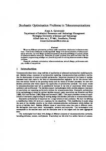
Fig. 5: Cumulative distribution functions of elapsed steps for each algorithm (ii: iterative improvement, sa: simulated annealing, ga: genetic algorithm) Given the similar number of steps, there exist the obvious differences in quality of results from each algorithm. As shown in Fig. 6, the genetic algorithm with high probability produces better solutions than the two other algorithms in both jamming impact and jamming energy conservation, while iterative improvement records the worst. Note that we compare 30 solutions each for iterative improvement and simulated annealing since each run bears only one solution. On the other hand, for the genetic algorithm only the Pareto fronts1 are depicted among the 60 individual solutions of the 40th generation in each run. Fig. 7 depicts the correlation of jamming impact and jamming energy conservation of each solution. Being consistent with the result from Fig. 6, genetic algorithm shows the best performance while iterative improvement shows the worst performance. For the purpose of comparison, we heuristically allocate the channel number to each jammer. Each jammer searches the nearest node which receives any packets from a flow. It jams on the same channel which the found node is receiving. If the flow to which the node belongs is already jammed by another jammer, it searches the next nearest node and repeats the same procedure. We allocate two-fold (2mW), four-fold (4mW), and eight-fold (8mW) of transmission power of wireless node to every flow-jammer and measure the jamming fitness for three cases. As shown in Fig. 7, the jamming energy conservation drops as the jamming power get increasing. However, it does not show much difference in jamming impact when varying power. In order to know how fast each algorithm approaches to the best solution, we also compare the progress of solution quality as elapsed steps increase in each algorithm in Fig. 8. At every 600 steps, we average the jamming fitness of 30 runs in each algorithm. Since only the Pareto fronts are collected in genetic algorithm, its jamming fitness in the initial step marks higher than the others. Iterative improvement shows the earliest saturation among three algorithms and stays in the lowest jamming fitness. Interestingly, iterative improvement 1 It is defined as the set of nondominated solutions among the possible solutions. In this case, the Pareto fronts are superior to the other individuals in terms of both jamming impact and jamming energy conservation. [8]

ii sa ga

0.8

jamming impact

cumulative distribution function

1

0.6 0.4 0.2 0

−0.4 −0.2

0 0.2 0.4 jamming impact

0.6

0.8

1 0.9 0.8 0.7 0.6 0.5 0.4 0.3 0.2 0.1

1

ii sa ga hs2w hs4w hs8w

0

jamming energy conservation

cumulative distribution function

1 ii sa ga

0.6 0.4 0.2 0 −2

1 0.8 0.6 0.4 0.2 0 −0.2 −0.4 −0.6 −0.8

6000

8000

ii sa ga hs2w hs4w hs8w

0

−1.5

4000 steps

(a) Jamming impact

(a)

0.8

2000

−1 −0.5 0 0.5 jamming energy conservation

2000

4000 steps

6000

8000

(b) Jamming energy conservation

(b)

Fig. 8: Progress of average jamming fitness for each step Fig. 6: Cumulative distribution functions of jamming fitness for each algorithm flow-jamming optimization by stochastic search algorithms through a network simulation. Our experimental results show that genetic algorithm produces the most efficient jamming configuration compared to the other algorithms. We expect that this work is used as a tool to analyze the effect of flowjamming attack over target network.

jamming impact

1 0.8 0.6 0.4 0.2 0 −0.2 −0.4 −2

ii sa ga hs2w hs4w hs8w −1.5

R EFERENCES 0 −1 −0.5 0.5 jamming energy conservation

1

Fig. 7: Correlation of jamming impact and jamming energy conservation (hs{x}w: heuristic strategy with {x}mW) shows better performance than simulated annealing in the 600th step. This is because simulated annealing allows the regression in quality of solution to avoid being confined in local maxima. Literally, it reduces the possibility of regression as it proceeds, thus quickly getting closer to the best solution. V. C ONCLUSION An attacker can use jammers to efficiently disrupt the flows in wireless network by using network-layer knowledge. In this paper, we study the optimization of flow-jamming attack. An existing work have introduced the identical problem and analyzed theoretical bounds for various cases by the non-convex optimization, but we focus on optimizing the flow-jamming attack over a channelized network model with stochastic search algorithms which provide us with more concrete realization and more tangible strategy. We reformulate the mathematical model of flow-jamming attack and the evaluation metric of jamming fitness. We demonstrate the

[1] D. J. Torrieri, Principles of Secure Communication Systems. Norwood, MA, USA: Artech House, Inc., 1985. [2] K. Pelechrinis, M. Iliofotou, and S. Krishnamurthy, “Denial of service attacks in wireless networks: The case of jammers,” Communications Surveys Tutorials, IEEE, vol. 13, no. 2, pp. 245 –257, quarter 2011. [3] W. Xu, K. Ma, W. Trappe, and Y. Zhang, “Jamming sensor networks: attack and defense strategies,” Network, IEEE, vol. 20, no. 3, pp. 41 – 47, may-june 2006. [4] G. Lin and G. Noubir, “On link layer denial of service in data wireless lans,” Wireless Communications and Mobile Computing, vol. 5, no. 3, pp. 273–284, 2005. [Online]. Available: http://dx.doi.org/10.1002/wcm.221 [5] D. J. Thuente and M. Acharya, “Intelligent jamming in wireless networks with applications to 802.11b and other networks,” in Proceedings of the 2006 IEEE conference on Military communications, ser. MILCOM’06. Piscataway, NJ, USA: IEEE Press, 2006, pp. 1075–1081. [6] P. Tague, D. Slater, G. Noubir, and R. Poovendran, “Quantifying the impact of efficient cross-layer jamming attacks via network traffic flows,” Network Security Lab (NSL), University of Washington, Tech. Rep., 2009. [Online]. Available: http://www.ee.washington.edu/research/ nsl/papers/TR005.pdf [7] H. Hoos and T. St¨utzle, Stochastic Local Search Foundation and Applications. Morgan Kaufmann Publishers, 2005. [8] A. E. Eiben and J. Smith, Introduction to Evolutionary Computing. Springer-Verlag, 2003. [9] OPNET Technologies, Inc., “OPNET Modeler 16.0.” [Online]. Available: http://www.opnet.com/solutions/network rd/modeler.html [10] T. S. Rappaport, Wireless Communications: Principles and Practice, 1st ed. Piscataway, NJ, USA: IEEE Press, 1996. [11] P. Husbands, “Distributed coevolutionary genetic algorithms for multicriteria and multi-constraint optimisation,” in Evolutionary Computing, ser. Lecture Notes in Computer Science, T. Fogarty, Ed. Springer Berlin / Heidelberg, 1994, vol. 865, pp. 150–165.