Stochastic Programming for Off-line Adaptive Radiotherapy

Preprint 0 (2009) ?–?

Stochastic Programming for Off-line Adaptive Radiotherapy MUSTAFA Y. SIR a,∗ , MARINA A. EPELMAN b , and STEPHEN M. POLLOCK b

a

Department of Industrial and Manufacturing Systems Engineering, University of Missouri, Columbia, MO 65211-2200, USA b Department of Industrial and Operations Engineering, The University of Michigan, Ann Arbor, MI 48109-2117, USA

In intensity-modulated radiotherapy (IMRT), a treatment is designed to deliver high radiation doses to tumors, while avoiding the healthy tissue. Optimizationbased treatment planning often produces sharp dose gradients between tumors and healthy tissue. Random shifts during treatment can cause significant differences between the dose in the “optimized” plan and the actual dose delivered to a patient. An IMRT treatment plan is delivered as a series of small daily dosages, or fractions, over a period of time (typically 35 days). It has recently become technically possible to measure variations in patient setup and the delivered doses after each fraction. We develop an optimization framework, which exploits the dynamic nature of radiotherapy and information gathering by adapting the treatment plan in response to temporal variations measured during the treatment course of a individual patient. The resulting (suboptimal) control policies, which re-optimize before each fraction, include two approximate dynamic programming schemes: certainty equivalent control (CEC) and open-loop feedback control (OLFC). Computational experiments show that resulting individualized adaptive radiotherapy plans promise to provide a considerable improvement compared to non-adaptive treatment plans, while remaining computationally feasible to implement. Keywords: adaptive radiotherapy, patient setup error, stochastic programming ∗

Corresponding author.

1

2

SIR, EPELMAN, AND POLLOCK / OFF-LINE ADAPTIVE RADIOTHERAPY

1.

Introduction

1.1. Background In 2007, an estimated 1.5 million people were diagnosed with cancer in the United States (Pickle et al., 2007). More than half of cancer patients in the US undergo radiotherapy (the use of radiation as a means for treating cancer) at some point during the course of their disease (Perez and Brady, 1998). In radiotherapy, radiation is delivered to cancerous regions in order to damage the DNA of the cells in the area being treated, interfering with their ability to divide and grow. As a result, radiation can be used to kill cancerous tumor cells and stop them from regenerating. Since both cancer and healthy cells are affected by radiation (see Stone et al., 2003, for effects of radiotherapy on normal tissue), any treatment plan should be designed in such a way that the radiation dose delivered to the tumor(s) is high enough to stop the cancer cells from regenerating, while simultaneously avoiding the delivery of excessive doses of radiation to surrounding healthy tissue. A “treatment protocol,” prescribed by a radiation oncologist, is a description of the desired dose to be delivered to the various regions of interest. Intensity-Modulated Radiation Therapy (IMRT), one of the most advanced and common forms of (external beam) radiotherapy, allows a significant amount of control over the characteristics of the radiation delivered by providing flexibility in the shapes of treatment beams, time of exposures, etc. (Webb, 2005). One beam can be represented by a decomposition into a grid of many “beamlets,” each of which can have a different intensity. As a result, radiation treatment plans can potentially conform much more precisely to the treatment protocol compared to traditional conformal radiotherapy techniques. Treatment planning, then, refers to activities involved in finding beamlet intensities which deliver doses of radiation that are as close to those specified by the treatment protocol as possible. These activities usually include repeated solutions of an optimization model embedded in specialized software, which, given a representation of patient anatomy via a collection of voxels (3-dimensional rectangular volume elements) and the treatment protocol, produces a solution in the form of beamlet intensities and resulting dose distribution, i.e., dose that would be delivered to each voxel. In recent years, optimization models used in this step of treatment planning have been an active area of research, and a wide variety of sophisticated models have been proposed (for an overview see, for instance, Shepard et al., 1999; Romeijn


3

et al., 2003; Lee et al., 2003; K¨ ufer et al., 2003; Kessler et al., 2005); proprietary models are embedded in a number of commercial treatment planning systems (see Petric et al., 2005). In clinical practice, once the treatment plan is decided on, it is delivered over a period of time as a series of small dosages called “fractions.” The number of fractions in a treatment is determined by the radiation oncologist (typically 5 treatments per week for a period of 4-9 weeks), and is part of the treatment protocol. Fractionation is used to increase tumor control probability and decrease damage to the healthy tissue surrounding the tumor by giving it time to recover (Thames and Hendry, 1987). 1.2. Uncertainty Many aspects of radiotherapy are subject to uncertainty. The most common uncertainty in radiotherapy is the position of the target(s) (i.e., the tumor(s) and other regions, such as lymph nodes, to be treated), and surrounding patient anatomy, with respect to the treatment beams. This uncertainty leads to delivery errors, i.e., differences between the dose distribution as calculated by a treatment plan and the actual dose distribution delivered to a patient. These errors can be classified as preparation (“systematic”) and execution (“random”) errors. Systematic errors include those occurring due to organ displacement on images and scans taken during the treatment planning session, tissue delineation (identification of voxels belonging to the targets and other organs and tissues), and equipment calibration. Random errors include those caused by movement during radiation delivery, day-to-day variation in the patient setup and equipment, and inherent inaccuracy of the delivery system (van Herk, 2004; Keller et al., 2003). Most existing optimization models used in treatment planning do not account for the uncertainties leading to these errors and typically produce plans containing sharp dose gradients between a tumor and its neighboring healthy tissue. As a result, it is possible, in some fractions, for the tumor to be in a low-dose radiation field while the healthy tissue regions may be exposed to a high-dose radiation field, resulting in complications and possibly failure of the treatment. Therefore, an “optimized” plan that does not take uncertainties into account may easily lose its advantage when it is subject to random shifts relative to a “nominal” position of the target and surrounding patient anatomy (e.g., a static position on the CT scanner) assumed in the treatment planning (Bortfeld

4


et al., 2004; van Herk, 2004; Lujan et al., 1999). Immobilization devices are commonly used to reduce uncertainty by helping patients maintain consistent positioning, both during treatment and from fraction to fraction (Bentel, 1999). Moreover, active breathing control devices are used to reduce the effects of respiratory movement (Wong et al., 1999; Koshani et al., 2006). However, even with these aids, discrepancies between the nominal and actual position of the target and surrounding patient anatomy are inevitable. The traditional treatment planning approach to dealing with uncertainty in radiotherapy is to expand the clinical target volume (CTV) by some amount (called a “margin”) to form a planning target volume (PTV) (ICRU, 1993, 1999). The width of the margin is typically set to be some number k times the standard deviation of the patient setup error and/or the internal organ motion (van Herk, 2004; van Herk et al., 2000; Sir et al., 2006). More recent approaches used in practice to account for geometrical uncertainties include convolution-based methods (Lujan et al., 1999; Chetty et al., 2003; Beckham et al., 2002) and Multiple Instance of Geometry Approximation (MIGA) (McShan et al., 2006). In convolution-based methods, uncertainties caused by daily setup procedures at the beginning of each treatment fraction, as well as the inter- and intra-fraction motion of the internal organs, are incorporated in dose calculations to calculate the average delivered dose values. MIGA, on the other hand, approximates the distribution of the random patient position by a distribution of a discrete random variable, and performs a dose deposition calculation for each of the possible discrete variable realizations, referred to as “setup instances” (see Section 2.2 for further details on MIGA). 1.3. Adaptive Treatment Planning As mentioned above, uncertainties in IMRT can lead to significant differences between the dose distribution calculated by an “optimal” treatment plan and the actual dose distribution delivered to a patient. With advanced technology (Schlegel et al., 2006), however, the position of the target and surrounding patient anatomy with respect to treatment beams can be measured during the treatment process using imaging devices such as electronic portal imaging device (EPID) (Herman et al., 2001), ultrasound (Keller et al., 2004), and CT scanner (Wu et al., 2006). Thus, fraction-to-fraction setup variation, long-term organ deformation, organ filling, patient respiration, and/or dose response can be mon-


5

itored and the treatment plan can be adapted to these measurements during the treatment course of an individual patient. Many techniques, referred to as Adaptive Radiation Therapy (ART), have been developed to exploit the additional information provided by the imaging devices (Yan et al., 1997a, 2000; Martinez et al., 2000; L¨of et al., 1995; Keller et al., 2003; Ferris and Voelker, 2004). In general, Yan (2006) describes ART as a system “designed to systematically manage treatment feedback, planning, and adjustment in response to temporal variations occurring during the treatment course.” In this paper, we concentrate on “off-line” ART, where measurements from imaging devices become available after the delivery of a fraction (Rehbinder et al., 2004; de la Zerda et al., 2007; Ferris and Voelker, 2004). Based on these measurements, treatment is then adjusted for future fractions. Online ART, on the other hand, attempts to adapt the treatment to variations during the delivery of a fraction (Mestrovic et al., 2007; Thongphiew et al., 2008). Unlike online ART, in off-line ART, a more thorough and careful analysis of measurement data can be performed after the delivery. Another advantage of off-line ART is that it does not affect the duration of a fraction, and therefore the patient throughput, since the treatment is not modified during the delivery. In the remainder of this paper, we will use the term ART to mean off-line ART. There have been two main directions in ART research. Most of the attention has been concentrated on the sequential refinement of knowledge about an individual patient by taking measurements of the patient’s fraction-to-fraction setup variation during the course of the treatment. These methods use well-established techniques such as Kalman filtering (Keller et al., 2003; Yan et al., 1997b) and Bayesian statistical methods (Lam et al., 2005; Sir, 2007) to “update” knowledge for correcting for systematic setup error (Keller et al., 2003; Bortfeld et al., 2002) and create individualized treatment margins (Yan et al., 2000; Keller et al., 2004). Imaging devices can also be used for reconstructing dose distributions actually delivered in a particular fraction (Partridge et al., 2002; McNutt et al., 1997), and therefore highlighting where the delivered treatment may not be as it was planned. This knowledge can then be exploited using a dynamic programming (DP), or stochastic control, framework. Ferris and Voelker (2004) formulate a DP model that attempts to compensate, over time, for movement of the patient and error in the delivery process. In this model, the target dose distribution for the remaining fractions of the treatment course is adjusted after each fraction,

6


taking into account the total dose that has already been delivered to each voxel (in effect, they modify the treatment protocol to be adhered to in planning for future fractions, but not the treatment plan, i.e., the beamlet intensities).1 Due to the size and complexity of the DP formulation, they resort to neuro-dynamic programming techniques to derive effective rule-of-thumb policies for modifying the target dose distribution. Wu et al. (2002) proposed a similar re-optimization framework for ART. Rehbinder et al. (2004), on the other hand, formulate ART as a linearquadratic (LQ) control problem which has a simple analytical recursive solution, in the form of the discrete-time Ricatti equation (Bertsekas, 2005). However, they do not constrain the beamlet intensities to be non-negative nor consider any additional constraints that may be required by the treatment protocol and/or the type of delivery machine. With these constraints, there is no analytical solution to the LQ control problem (Sir, 2007, Chapter 4). In this paper, we develop a similar optimization framework that exploits the dynamic nature of radiotherapy and information gathering by adapting the treatment plan in response to variations measured during the treatment course of an individual patient, while incorporating, when appropriate, non-negativity and other constraints. We use and compare two approximate dynamic programming schemes, namely certainty equivalent control (CEC) and open-loop feedback control (OLFC), to find beamlet intensities for each fraction of the treatment. Depending on the scheme used, the optimization problem for finding the beamlet intensities can be posed as a linear programming or stochastic programming problem, the latter solved by a cutting plane algorithm. We analyze the structure of optimization problems arising in computing these policies when arbitrary convex cost functions and convex constraints are used. We then specialize our analysis to the case when the objective and constraint functions are based on equivalent uniform dose (EUD) functions commonly used in assessment of IMRT treatment plans. The paper is organized as follows: In Section 2 we give the basics of modeling radiation delivery and uncertainty in patient positioning. In Section 3 we describe the objective and constraint functions we use in optimization problems 1

“Target dose,” i.e., the dose distribution treatment planners aim to deliver in the remaining fractions of the treatment, should not be confused with the target volume, i.e., the tumor(s) and other tissues to be treated to a high dose of radiation.


7

for finding beamlet intensities. We then discuss how approximate dynamic programming schemes CEC and OLFC are utilized in adaptive radiation treatment planning. In Sections 4 and 5 we formulate optimization problems for CEC and OLFC, respectively, and discuss solution techniques for the resulting problems. Finally, Section 6 presents several numerical examples comparing the performance of different control policies via simulation. 2.

Modeling radiation delivery and uncertainty in fractionated IMRT

2.1. Setup position in a fraction In every fraction, the position of the patient (referred to as the “setup position”) is characterized by the three-dimensional random vector 



X    X≡ Y  Z

representing the position of an anatomical reference point with respect to an arbitrary fixed origin in the room coordinate system. A realization x of the random vector corresponds to a shift of the whole set of voxels rigidly, without any rotation or organ deformation, so that the anatomical reference point is located at x. X is typically assumed to have a three-dimensional Normal distribution with probability density function (pdf) given by 3

1

1

fX (x; m, v) = (2π)− 2 |v|− 2 e− 2 (x−m)

Tv−1 (x−m)

.

(1)

where m ∈ R3 is the mean vector and v is the 3 × 3 covariance matrix (Lam et al., 2005; Schewe et al., 1996). For simplicity, in the remainder of this paper, we assume that there is no sys'

(T

tematic error (i.e., m = 0 0 0 ). This is not a very strong assumption as most clinics use daily localization and correction procedures primarily aimed at eliminating systematic errors (Lam et al., 2007). Although these procedures along with immobilization and active breathing control devices help reducing random errors, discrepancies between the nominal and actual position of the patient anatomy cannot be eliminated. Sir (2007) discusses applications of Bayesian statistical methods in the presence of both systematic and random errors.

8


When there are N remaining fractions in the treatment, the setup positions X1 , X2 , . . . , XN are independent and identically distributed (iid), where Xn is the setup position in the nth upcoming fraction. As implicitly assumed above, we consider only random setup errors with rigid body motion in this paper. In theory, one can also include rotations and organ deformations in the model of uncertainty. However, this might signicantly complicate the problem because of (i) the complexity (or even unavailability) of appropriate stochastic models for changes in patient anatomy due to organ deformation and weight loss; and (ii) the fact that realizations of such changes are likely not iid over the course of the treatment. Conceptually, the approximate dynamic programming framework described in the remainder of this paper can be extended to address these issues, possibly at the expense of substantially increased computation times. 2.2. Dose models, dose deposition matrix and MIGA Recall that in IMRT optimization the tissue subjected to radiation is represented by a set of voxels, and radiation beams are represented by a set of beamlets. Using physics principles, a dose deposition matrix can be generated by computing how a unit-intensity beamlet will deposit energy to voxels as it travels through the body of the patient. In particular, with v the number of voxels and b the number of beamlets, D ∈ Rv×b + is the dose deposition matrix with elements dij defined as the dose delivered to voxel i by beamlet j at unit intensity. Then if w ∈ Rb+ is the vector of beamlet intensities used in a fraction, the vector of doses delivered to the patient is Dw ∈ Rv+ . We assume that dose is additive, i.e., dose delivered to a voxel in the course of the entire treatment is computed as the sum of doses delivered to this voxel in each fraction of the treatment. Although dose additivity is a common assumption (Chu et al., 2005; Ferris and Voelker, 2004), other dose models have been proposed to reflect the biological effects of fluctuations in dose delivery over fractions (Bortfeld and Paganetti, 2006). Many aspects of the analysis we present can be extended to these dose models. These extensions, however, fall outside the scope of this paper. The dose deposition matrix depends on the patient’s position with respect to the beams. We therefore define the mapping D(x) : R3 → Rv×b as the dose + deposition matrix when the anatomical reference point on the patient is at room


9

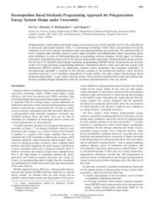
coordinate x. When the position of the anatomical reference point is the random variable X, the dose deposition matrix is the random matrix D(X). Since the calculation of D(·) is usually a subroutine in the treatment planning system and X is typically assumed to have a continuous distribution, there is no convenient way to use D(X) directly in subsequent analysis. Therefore, an approximation for the distribution of D(X) is in order. One method, known as the “multiple instance of geometry approximation” (MIGA) (McShan et al., 2006), is to approximate the distribution of setup position in each fraction with a discrete distribution over “setup instances.” Suppose that there are K setup instances used in the approximation, each of which is assigned probability pk , k = 1, . . . , K, of occurring. The k th setup instance is characterized by xk ∈ R3 and corresponds to a shift of the voxels, so that the anatomical reference point is located at xk . Figure 1 shows an example of a MIGA distribution for K = 7. The parameters of MIGA are selected to approximate the true distribution of X (1). A dose deposition matrix calculation can be performed for each setup instance of MIGA, storing the resulting matrices D(x1 ), D(x2 ), . . . , D(xK ). Thus the random dose deposition matrix D(X) is approximated by another random ) having the probability mass function (pmf) matrix D, ) = D

3.

   D(x1 ), with probability p1 ,     D(x2 ), with probability p2 ,

..   .    

.. . D(xK ), with probability pK .

(2)

Optimization models in adaptive treatment planning

As mentioned in the introduction, in the process of IMRT treatment planning, an optimization problem is often solved to obtain a treatment plan that optimizes a cost function that serves as a performance measure for comparing feasible plans that meet the constraints of the treatment protocol. A wide variety of optimization models have been proposed in medical and operations research literature. In this section, we will outline the structure of the objective function and constraints used in our models, and conclude the section with an outline of two approximate dynamic programming schemes for ART.

10


0.083 0.083

0.5

0.083

0.083

0.083 0.083

Figure 1. Multiple Instance of Geometry Approximation. The centers of the circles represent the position of each setup instance; the size of the circles and the numbers inside are the probabilities for each setup instance.

3.1. Objective function Let d ∈ Rv+ be the total dose delivered at the end of the treatment course. The cost function we will use to evaluate treatment plans is of the form f (d) ≡

L .

rl fl (d),

l=1

where L is the number of treatment criteria considered in the treatment plan, fl (d), l = 1, 2, . . . , L, are convex functions of d, and rl ≥ 0, l = 1, 2, . . . , L. Each function fl (d) represents a criterion used as a measure of performance for a single treatment region. Note that there might be several criteria for each treatment region. Therefore, L might be greater than the number of treatment regions in a treatment plan. A possible functional form for fl (d) is defined through an Equivalent Uniform Dose (EUD) function which summarizes a heterogenous dose distribution over a specific treatment region (a target or a healthy organ or tissue) by a single value: the uniform dose that would have the same biological effect on the region. The generalized EUD formula (Niemierko, 1999) is EUDa (d) =

/

1 . (di )a |S| i∈S

01/a

,

where S is the set of voxels of the treatment region, d is the delivered dose vector,


11

and a is a region-specific parameter. We make the following observations (Choi and Deasy, 2002): • As a → ∞, EUDa (d) approaches maxi∈S di . This function is suitable for a region of healthy organ tissue with a serial structure, in which damage to any part of the organ results in the failure of the entire organ. • When a = 1, EUDa (d) is equal to the average dose delivered to all voxels in 1 1 the treatment region, i.e., |S| i∈S di . This function is suitable for a region of healthy organ tissue with a parallel structure, in which even if some part of the organ is damaged, the undamaged portion still performs the functions of the organ. • As a → −∞, EUDa (d) approaches mini∈S di . This function can be utilized in cost functions for tumors. |S|

Notice that EUDa (·) defined over R+ is convex when a > 1, concave when a < 1, and linear when a = 1; see Choi and Deasy (2002). An alternative expression for EUD, referred to as “linear EUD” and denoted in the literature by αEUD, was presented in Thieke et al. (2002). αEUD is a convex combination of appropriate generalized EUD functions of Niemierko (1999), namely: • For tumors, αEUD(d) = α min di + (1 − α) i∈S

• For organs and healthy tissue, αEUD(d) = α max di + (1 − α) i∈S

1 . di . |S| i∈S

(3)

1 . di . |S| i∈S

(4)

In the above, α ∈ [0, 1] is a region-specific parameter. Note that the function in (3) is concave in d, while the function in (4) is convex. These formulas are attractive because they give rise to linear re-optimization problems as demonstrated in the rest of this paper (see also (Craft et al., 2005)). 3.2. Constraints Constraints typically imposed in treatment planning include: • Nonnegativity constraints for beamlet intensities: w ≥ 0.

(5)

12


• General constraints of the form gm (d) ≤ 0,

m = 1, 2, . . . , M,

(6)

where the convex functions gm (d) represent some measures of performance relevant to the outcome of the treatment but not incorporated into the cost function. In general, we will consider three types of treatment regions: the tumor(s), referred to as the clinical target volume (CTV), organ(s)-at-risk (OAR), and healthy (also called normal) tissue. We denote the set of voxels in the CTV by St , the set of voxels in the OAR by So , and the set of healthy tissue voxels by 2 2 Sh . S ≡ St So Sh denotes the set of all voxels. The constraints of (6) include lower and upper bound constraints: lt ≤ di ≤ ut , di ≤ uo ,

di ≤ uh ,

i ∈ St ,

(7)

i ∈ Sh ,

(9)

(8)

i ∈ So ,

where ut , uo and uh are the upper bounds on the total dose to be delivered to voxels in the CTV, OAR and healthy tissue, respectively, and lt is the lower bound on the dose to be delivered to voxels in the CTV. In addition, constraints on linear EUDs in different treatment regions are included: αEUDt (d) ≡ αt min di + (1 − αt ) i∈St

1 . di ≥ Lt , |St | i∈S

(10)

t

1 . αEUDo (d) ≡ αo max di + (1 − αo ) di ≤ Uo , i∈So |So | i∈S

(11)

αEUDh (d) ≡ αh max di + (1 − αh )

(12)

o

i∈Sh

1 . di ≤ Uh , |Sh | i∈S h

where Lt is the lower bound on αEUD in the CTV, and Uo and Uh are upper bounds on αEUD in the OAR and healthy tissue, respectively. 3.3. Approximate dynamic programming for adaptive radiation treatment ) is the Suppose there are N fractions remaining in the treatment, and d ) = 0 at the beginning of the total dose delivered in the prior fractions (we set d treatment). Let w1 , . . . , wN be the beamlet weight vectors used in the remaining


13

fractions. Then the (random) dose delivered at the end of the treatment is given by )+ d=d

N .

D(Xn )wn .

n=1

The Adaptive Radiation Therapy problem (with N remaining fractions) can then be stated as the problem of minimizing the expectation 3 /

)+ EX1 ,...,XN f d

N .

n=1

D(Xn )wn

04

over w1 , . . . , wN , subject to the constraints (5) and (6) with the qualification that wn is selected with the knowledge of realizations x1 , . . . , xn−1 , and hence ) + D(x1 )w1 + · · · + D(xn−1 )wn−1 . the dose d Two challenges are presented by the above optimization problem. Firstly, the presence of constraints (6) makes the standard dynamic programming algorithm inapplicable. Without these constraints, the dynamic programming algorithm is theoretically applicable, but becomes computationally intractable. To address these challenges we apply and compare the performance of two techniques of approximate dynamic programming: certainty equivalent control and open-loop feedback control (see, for example, Bertsekas, 2005, for details). • Certainty equivalent control (CEC): For the purposes of optimization, future stochastic fraction-to-fraction setup positions are replaced by a nominal deterministic one (e.g., the MIGA setup instance corresponding to the most likely position of the patient, or to the expected value of the random variable X). The expression for the total dose delivered is simplified to )+ d=d

N .

n=1

) + N Dnom w. Dnom w = d

where Dnom is the dose deposition matrix at the nominal setup position. The optimization problem for determining the beamlet intensities in this scheme becomes a deterministic optimization problem; the details of its formulation are described in Section 4. • Open-loop feedback control (OLFC): The stochastic nature of the doses to be delivered in future fractions is incorporated into the optimization, but it is assumed that no further measurements

14


will be taken, and therefore no further adjustment will be made to the plan. The resulting treatment plan design problem becomes that of minimizing the expected cost for the remaining fractions of the treatment course, and can be solved using stochastic programming techniques. The expression for the total dose delivered becomes )+ d=d

or, using MIGA,

N .

D(Xn )w,

n=1

)+ d=d

N .

n=1

) n w, D

) n is the dose deposition matrix in the nth fraction with pmf given where D by (2). The optimization problem for determining the beamlet intensities in this scheme becomes a stochastic programming problem; the details of its formulation are described in Section 5.

The adaptive radiation treatment planning proceeds as follows: with N frac) is observed/calculated, and the optimization tions remaining, the dose-to-date d problem for determining beamlet intensities is formulated in accordance to the approximate dynamic programming technique employed. The beamlet intensities obtained in the optimization are used for treatment in the next fraction, during which the setup position of the patient is observed and the dose-to-date vector is updated. The process is then repeated until the end of the treatment is reached. We will compare the performance of the CEC and OLFC schemes used within ART framework in Section 6. 4.

The re-optimization problem for CEC

In CEC, at every future fraction the dose deposition matrix is assumed to be Dnom . The resulting re-optimization problem becomes a deterministic open-loop control problem from the present fraction to the end of the treatment course: L .

rl fl (d)

(13)

) + N Dnom w subject to d = d

(14)

min f (d) ≡ w,d

l=1

gm (d) ≤ 0,

m = 1, 2, . . . , M

(15)


15

(16)

w≥0

Since the functions fl (d) and gm (d) are convex in d and d is an affine function of w, the problem (13)-(16) is a convex optimization problem. In the numerical examples that follow, we use EUD-based cost function f (d) = −rt αEUDt (d) + ro αEUDo (d) + rh αEUDh (d)

(17)

and constraints given in equations (7)-(12). Using standard transformation techniques, the resulting optimization problem can be rewritten as min

d,w,yt ,yo ,yh ,µt ,µo ,µh

5

−rt (αt yt + (1 − αt )µt ) + ro (αo yo + (1 − αo )µo ) 6

+ rh (αh yh + (1 − αh )µh ) ) + N Dnom w subject to d = d

(18) (19)

w≥0

(20)

yt ≤ di , i ∈ St 1 . µt = di |St | i∈S

(21)

di ≤ ut ,

(24)

CTV constraints: (22)

t

yt ≥ lt

i ∈ St

(23)

αt yt + (1 − αt )µt ≥ Lt

(25)

yo ≥ di , i ∈ So 1 . µo = di |So | i∈S

(26)

αo yo + (1 − αo )µo ≤ Uo

(29)

yh ≥ di , i ∈ Sh 1 . di µh = |Sh | i∈S

(30)

αh yh + (1 − αh )µh ≤ Uh

(33)

OAR constraints:

(27)

o

yo ≤ u o

(28)

Healthy tissue constraints: (31)

h

yh ≤ u h

(32)

16


Note that the optimization problem (18)-(33) is a linear program (LP), which can be solved efficiently. 5.

The re-optimization problem for OLFC

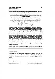
In OLFC, the stochastic nature of the doses delivered in future fractions is incorporated into the re-optimization. However, it is assumed that no further measurements of the delivered dose will be taken, and therefore no further adjustment will be made to the beamlet intensities (Sir, 2007, Chapter 4). The goal is to find the beamlet intensity vector which minimizes expected cost from the present fraction to the end of the treatment course and does not violate the constraints under any realization of the dose deposition matrices. This section discusses the resulting re-optimization problem when MIGA with K setup instances is used as the approximate model of uncertainty and how it can be solved using stochastic programming techniques (Birge and Louveaux, 1997; Ruszczynski and Shapiro, 2003; Diwekar et al., 2002). 5.1. Scenarios and the re-optimization problem formulation To derive the stochastic programming formulation for OLFC, we introduce the concept of a scenario: a scenario represents a sequence of setup positions of the patient in all (remaining) fractions. Using a MIGA model with K setup instances, with N remaining fractions, the number of scenarios is K N (see Figure 2). In view of the dose additivity assumption, to calculate the dose delivered to the patient in a particular scenario, it is sufficient to specify the number of times each MIGA setup instance occurs in this scenario. We thus refine the concept of a scenario: a scenario ξ is characterized by K nonnegative integers 1 N1 (ξ), N2 (ξ), . . . , NK (ξ) such that K k=1 Nk (ξ) = N , where Nk (ξ) is the number of times the setup instance k occurs in the remaining N fractions. The probability of this scenario occurring is given by q(ξ) = N !

N (ξ) K 7 pk k .

k=1

Nk (ξ)!

Let Ω be the set of all scenarios defined this way. Table 1 shows elements of Ω for +K−1)! K = 3 and N = 5. It can be shown that |Ω| = (N (K−1)!N ! , growing significantly slower than K N as a function of either K or N .


Fraction 1

Fraction n

Fraction 2

17

Fraction N

Figure 2. Illustration of the scenario tree with three setup instances (K = 3). Table 1 List of scenarios Ω for K = 3 and N = 5.

N1 N2 N3

1

2

3

4

5

6

7

8

9

0 0 5

0 1 4

0 2 3

0 3 2

0 4 1

0 5 0

1 0 4

1 1 3

1 2 2

Scenario index, ξ 10 11 12 13 14 1 3 1

1 4 0

2 0 3

2 1 2

2 2 1

15

16

17

18

19

20

21

2 3 0

3 0 2

3 1 1

3 2 0

4 0 1

4 1 0

5 0 0

We denote by D(ξ) the total dose deposition matrix under scenario ξ: D(ξ) ≡

K .

Nk (ξ)D(xk ),

k=1

and for every ξ ∈ Ω, we define ) + D(ξ)w), l = 1, 2, . . . , L, • f8l (w; ξ) ≡ fl (d

• f8(w; ξ) =

1L

8

l=1 rl fl (w; ξ),

and

) + D(ξ)w), m = 1, 2, . . . , M . • g8m (w; ξ) ≡ gm (d

18


Using the above notation, the re-optimization model for OLFC is a stochastic programming problem given by min w

.

ξ∈Ω

q(ξ)f8(w; ξ)

subject to g8m (w; ξ) ≤ 0, w ≥ 0.

(34) ∀m,

∀ξ

(35) (36)

Note that the functions f8(w; ξ) and g8m (w; ξ) are convex functions of w, and thus (34)-(36) is a convex optimization problem. The number of constraints in (35) can be significantly reduced by considering only basic scenarios. We define a basic scenario ξk" , k = 1, 2, . . . , K, to be one in which the patient will be in setup instance k in all of the remaining fractions of the treatment course (i.e., Nk (ξk" ) = N , Nj (ξk" ) = 0 for j *= k). Under this scenario the total dose deposition matrix is given by D(ξk" ) ≡ N D(xk ). For example, in Table 1, the basic scenarios are 1, 6 and 21. Proposition 5.1 shows that problem (34)-(36) is equivalent to min w

.

ξ∈Ω

q(ξ)f8(w; ξ)

subject to g8m (w; ξk" ) ≤ 0, w ≥ 0.

(37) ∀m,

∀k

(38) (39)

Proposition 5.1. Optimization problems (34)-(36) and (37)-(39) are equivalent. Proof of Proposition 5.1. The optimization problems have identical objective functions, and the feasible region of the former is easily seen to be contained in the feasible region of the latter. Suppose that w ≥ 0 satisfies (38). Consider an arbitrary scenario ξ ∈ Ω which is characterized by K nonnegative integers N1 , N2 , . . . , NK such that 1K k=1 Nk = N . Under this scenario, the total dose delivered at the end of the treatment course is equal to )+ d

K .

k=1

Nk D(xk )w.


19

Then, for any m, g8m (w; ξ) = gm

/

)+ d

K .

Nk D(xk )w

k=1

0

/K 0 : . Nk 9 ) d + N D(xk )w = gm k=1

≤ =

K . Nk

k=1 K .

N

N

9

) + N D(x )w gm d k

Nk g8m (w; ξk" ) ≤ 0, N k=1

:

where (40) follows by convexity of gm . Thus w satisfies (35).

(40)

!

As mentioned above, the framework presented in this paper can be easily extended to more realistic dose models, which take into account the biological effects of fluctuations in dose delivery over fractions. For example, it can be readily shown that the above proposition is still valid if the additive dose model is replaced with a linear-quadratic dose model (Bortfeld and Paganetti, 2006; Thames and Hendry, 1987) under the mild assumptions that • the fractions are temporally well separated;

• the constraint functions gm are convex functions of the biologic effect vector and monotonic in each argument (e.g., penalizing the deviations beyond a certain threshold). 5.2. Cutting plane algorithm The problem in (37)-(39) is a convex optimization problem. The difficulty in solving this problem lies in the functional form of the objective function, which can become intractable when the number of scenarios is large. Therefore, we will solve this problem by employing a cutting plane approach. In the remainder of this section, we will closely follow the terminology and notation of Ruszczynski and Shapiro (2003). They present a general cutting plane algorithm similar to Kelley’s cutting plane method (Kelley, 1960) in which a convex optimization problem is approximated by a master program where • the objective function is a convex piece-wise linear function which is a lower bound on the objective function of the original problem, and

20


• the feasible region is a polyhedron which contains the feasible region of the original problem. The master problem is solved using linear programming techniques, and its solution is used to generate cuts, i.e., linear inequality constraints that improve the approximation by either tightening the lower bound on the objective function, or reducing the size of the polyhedron containing the feasible region. The cuts are added to the master problem, and the process is repeated. In solving the problem (37)-(39), only objective function cuts will be generated, since the feasible region will be represented exactly in the master problem. We denote the set of all subgradients of a convex function h : Rn → R at a point x0 ∈ Rn (also called the subdifferential) by ∂h(x0 ), that is, z ∈ ∂h(x0 ) ⇔ h(x) − h(x0 ) ≥ zT(x − x0 ), ∀x ∈ Rn . For example, if h(·) is differentiable, its gradient at x0 is a unique element of the subdifferential, i.e., ∂h(x0 ) = {∇h(x0 )}. Suppose that w% satisfies (38)-(39) and let zl (w% , ξ) ∈ ∂ f8l (w% ; ξ). Then, from the definition of subgradient, for any w, L . l=1

i.e., z(w% ; ξ) ≡

rl f8l (w; ξ) ≥ L . l=1

L . l=1

rl f8l (w% ; ξ) +

L . ; l=1

Stochastic Programming for Off-line Adaptive Radiotherapy

Stochastic Programming for Off-line Adaptive Radiotherapy

Suggest Documents