Mar 1, 1985 - of the Langevin equation into an eigenvalue problem as the frame- work of the stochastic simulation of quantum systems. The potential of the ...
PHYSICAL REVIEW B
VOLUME 31, NUMBER 5
1
MARCH 1985
Stochastic simulation of quantum systems and critical dynamics T. Schneider, M. Zannetti, * and R. Badii IBM Zurich Research
I.
aboratory, 8803 Riischlikon, Switzerland (Received 20 August 1984)
We propose transformation of the Langevin equation into an eigenvalue problem as the framework of the stochastic simulation of quantum systems. The potential of the method is illustrated by numerical results for the low-lying energy levels of one-particle systems and coupled harmonic oscillators. Another application is the relationship between the dynamics of a d-dimensional system evolving according to the Langevin equation, an associated d-dimensional quantum system, and its (d+1)-dimensional classical counterpart. On this basis we relate the critical dynamics to the static properties of an associated quantum system and its (0+1)-dimensional classical analog. This then leads to equalities and scaling relations between the static and dynamic critical exponents. As a specific example, we treat the time-dependent Ginzburg-Landau model without conservation laws. In the large-n limit, the critical dynamics is traced back to Gaussian (tricritical Lifshitz) behavior of the associated (0+1)-dimensional classical model. The static exponents describing the critical dynamics are determined, however, by the crossover from Lifshitz to Gaussian (tricritical Lifshitz) behavior.
I. INTRODUCTION Stochastic processes, via Monte Carlo techniques' and the Langevin equation, ' are currently widely used in many areas of physics as a tool for numerical simulations. In these techniques stochastic processes are introduced with the, requirement that the associated equilibrium density coincides with the probability density of a quantum or classical system which is to be simulated. The equation of motion of the stochastic process can then be used to calculate expectation values of interest in terms of time averages. In this paper we present an alternative technique to simulate a quantum system, based on the Langevin equation. A preliminary account was given in Ref. 5. This is achieved by considering the Fokker-Planck equation associated with the Langevin equation. In fact, the FokkerPlanck equation can be reduced to the Schrodinger equation by appropriately choosing the variance of the random force. As a result, a system evolving according to the Langevin equation and specified by its potential energy 8', is related to a quantum system with potential energy Consequently, ground-state V, where V(8') is known. properties and the energy spectrum of the quantum system can then be investigated by simulating correlation functions in the stationary Langevin process. Another interesting aspect of this relationship between the Langevin equation and an associated quantum problem stems from the fact that the variables entering the quantum system are canonically conjugate. Accordingly, the quantum system can be mapped on a ( d + 1)dimensional classical model. On this basis, it becomes possible to relate the critical dynamics of a d-dimensional system evolving according to the Langevin equation to the static critical properties of the associated quantum system and in turn to the static critical properties of the corre31
sponding (d + 1)-dimensional classical system. This then leads to equalities and scaling relations between the dynamic and static critical exponents of these models. As a specific e'xample, we consider the n-component model without conservation laws, and Landau-Ginzburg construct the associated (d +1)-dimensional model. It is a highly anisotropic system with complex critical behavior. We study this model in the large-n limit and find a critical surface containing a line of Lifshitz points and a line of tricritical points intersecting at a Lifshitz mult&critical point. The approach to dynamic criticality in the d-dimensional system is then related to the static properties of a (d + 1)-dimensional system along a special trajectory in the parameter space, which terminates at the Gaussian (Lifshitz tricritical) point. The static and dynamic critical exponents of the d-dimensional model are then related to the static critical exporients of the (d + 1)-dimensional system by means of the Lifshitz-toGaussian (tricritical Lifshitz) crossover. Accordingly, the critical dynamics of the time-dependent Ginzburg-Landau model without conservation laws, is traced back to CzaussLifshitz) behavior in the associated ian (tricritical (d+1)-dimensional model. The static exponents describing the critical dynamics, however, are determined by the (Lifshitz tricritical) crossover from Lifshitz-to-Gaussian behavior. The paper is organized as follows. In Sec II we sketch the relationship between the model evolving according to the Langevin equation, the associated quantum system, and its (d +. ]. )-dimensional classical counterpart. Section III is devoted to explori. ng the potential of simulating quantum systems in terms of the Langevin process. We treat one-particle systems and a linear chain of coupled harmonic oscillators, allowing assessment of the accuracy of the method. The mappings of the critical dynamics of a d-dimensional Langevin process without conservation of an associated dlaws onto the static properties 2941
1985
The American Physical Society
T. SCHNEIDER, M. ZANNETTI, AND R. BADII
2942
dimensional quantum model and its (d+1)-dimensional classical counterpart are presented in Sec. IV.
and denoting
= —aW +r)(t),
(2. 1)
Bx
—
t') .
(x(t)x(0)) =
+
p
o.
Bp
reducing for t
In the stationary equilibrium independent solution —2 8'/o.
state, it admits
(2.4)
By invoking the transformation
p(x, t) =p,'q %(x, t),
(2.5)
it reduces to o 8 0'
O'P
QX
8' and
The potentials tion 20
V are related by the Riccati equa-
188'
2
aw
(2 6)
2
(2.7)
2'
c)x
The associated eigenvalue problem,
('e,
as
(2. 12)
t
two-time
ix') (2. 13)
=0 to
f pox dx .
(2. 14)
Ergodicity of the Langevin process implies that these quantities can also be obtained from the solution of the Langevin equation (2. 1) in terms of time averages, namely,
(x (t)x(0) ) =
1
lim n
n
m
—t —tm
x (t')x (t'+ t)dt'
X f,
(2. 15)
and
( x')
=
the tirne-
peq-~
(x)e yp(x') y
(O~x ~m)
(
(x(0)x(0)) =(x ) =
(2.2)
(2.3)
(x')
f dx f dx'xx'p„(x')p(x,
=g
density is
88'
condition
reducing for t =0 to Eq. (2. 11). Stationary correlation functions can then be expressed as
The associated Fokker-Planck equation for the probability
8
q
0
where q is a Gaussian random force with
( g(t) ) =0, (g(t)g(t') ) =o6(t
with this initial
g,
~
p(x, t ~x')=go(x)
In this section we sketch the relation between the Langevin-Fokker-Planck and the Schrodinger equations. This relationship allows estimation of quantum properties from the time evolution of an associated system satisfying the Langevin equation or vice versa. Moreover, it connects the dynamics of a d-dimensional Langevin system with a d-dimensional quantum system which in turn can be mapped on a (d +1)-dimensional classical system. To sketch the method, we first consider a one-particle system with time evolution defined by the stochastic differential equation of the Langevin type
dx dt
the solution
p(x, t x'), we obtain
II. BASIC FORMALISM
x=
31
lim
t„—t ~m
t„—tm
f
tm
x'(t')dt' .
(2. 16)
The long-time behavior of the Langevin process then proA, ~ estimates for the lowest eigenvalues with &O~x ~m, &~O, from
vides
(x~(t)x~(0))
)
(0
~
x& m ~
)
(
e
(2. 17)
This set of equations constitutes the framework for the correspondence between a Langevin process and a quantum problem. In fact, considering the Schrodinger equation
i
Qgg
3t
=— A%',' $
fg
A=-
g2
g2
2pyz
()x2
+ V(x),
(2. 18)
and setting
%'- e
—iA,
t
y~ (x),
(2. 19)
we obtain the eigenvalue
problem
r
0 BX
+~
gm =~mV'm
yields a non-negative
~0=0
(2.8)
~
BX2
energy spectrum, with 1/2
~
(2.9)
Wo=peq
The general solution of the Fokker-Planck then be expressed as 2 p(x, t) =(pa+go
g
m=1
c p e
t
equation
can
(2. 10)
By invoking the initial condition
x'), p(x, o) =6(x —
(2. 11)
1— + —V(x)
(2.20)
which is identical to the corresponding Fokker-Planck pressions, Eqs. (2.6) and (2.8), provided that
t~it,
o. =— fPl
—V(x)= V(x) . fi
ex-
(2.21)
From Eqs. (2. 13)— (2. 17) it then follows that the groundstate properties of this quantum system can be obtained as time averages from the solutions of the Langevin process (2. 1). For the purpose of numerical this simulation, correspondence might be used in two ways.
STOCHASTIC SIMULATION OF QUANTUM SYSTEMS AND. .
31
(i) The potential V entering the quantum problem is constructed from a given W by means of the Riccati equation (2.7). W entering the (ii) For a given V, the potential Langevin process must be obtained from an independent method of solution of the Schrodinger equation for the ground-state. In case (ii), W might be obtained by solving the Riccati equation (2.7), which now reads 2
1
18W
20
Bx
V(x) —A, p ——
(2.22)
In general, A. o does not vanish and must be determined from the Schrodinger equation. From the corresponding ground-state wave function W might then also be obtained as
W= —O. in@0 .
(2.23)
In fact, substitution of this expression into Eq. (2.22) Moreover, the eigenyields the Schrodinger equation. values in Eqs. (2. 13) and (2. 17) must then be replaced by —+A, =A, —A, p. The ground-state eigenvalue and eigenfunctions of the quantum problem defined by V(x) are denoted by A, o and cpo, respectively. The connection between the Langevin equation and the quantum problem can also be illustrated in terms of the probability distribution over sample paths, allowing a simpler generalization to the case of infinitely many degrees of freedom. From the Feynman-Kac formula, this is given by
dp
f
q[x(t)]-exp —
+ oo 2Q
oo
+ V(x)
dt Dx(t)
(2.24) where
Dx(t) is the usual formal measure on paths, and
V(x) is given by Eq. (2.7). Now, setting o =A'/m, the above expression is recognized as the probability measure arising in the Euclidean (imaginary time) representation of the ground-state expectations for the quantum problem with potential V(x). Finally, note that Eq. (2.24) can also be interpreted as the Gibbs equilibrium measure of a classical system in one space dimension, yielding for the partition function the expression
Z- f Dx (t)exp —f +
oo
+V
(2.25)
dt
The method is easily extended to X-particle systems. The laws is conservation without stochastic dynamics described by a set of coupled Langevin equations, which now read BX~
+pl(t) .
The N-independent &Rl(t)
&
=o,
(2.26)
-—
Gaussian noise sources satisfy &rll(t)rlt
(t')
&
= o5«5(t
t') .
(2.27)
As in the one-particle case, the associated Fokker-Planck equation leads to an eigenvalue problem [Eq. (2.8)], which
.
now reads
0 2
BXI
+ V(xl~ . . ~xn)
(2.28)
~nq'n
qn
of W by the Riccati equation
where Vis given in terms
aW
1
~B W
(2.29)
BXI
In terms of these eigenfunctions and eigenvalues, tion functions can be expressed as
C(q, t) = &x (q t)x ( — q 0) )
=g
(
&0
(
x (q)
(
n
correla-
) [ 'e (2.30)
where
x(q, t)=
ge'&'[x, (t)
&x,
. )] —
(2.31)
Correlation functions might also be obtained from the solution of the Langevin equations (2.26) in terms of time averages [Eqs. (2. 15) and (2. 16)],
x(q, t)x ( — q, 0) ) = —lim tn t — tm ~~t n — t— tm t — t x (q, t')x ( —l, t && 1
&
f
+ t')dt' . (2.32)
The long-time behavior then provides, as in the oneparticle case [Eq. (2. 17)], estimates for the lowest eigenvalues and the corresponding matrix element. Following the steps outlined in the one-particle case (2.21)], we obtain from Eq. (2.28) for the [Eqs. (2. 18)— Hamiltonian of the associated quantum system the expression
fi
2m
I
, +V=+I
gX(
mxl 2A
+v
(2.33)
the same eigenvalues and eigenfunctions as the Fokker-Planck eigenvalue problem (2.28), provided that o. =fz/m. Accordingly, the ground-state properties of this X-particle quantum system can be obtained from the solution of the Langevin equations (2.26) in terms of time having
averages. For the purpose of numerical simulation and in full analogy to the one-particle case, this correspondence can be used in two ways. (i) The potential V entering the quantum problem is constructed from a given 8' by means of the Riccati equation (2.29). (ii) For a given V, the potential W, entering the Langevin equation, must be obtained from an independent method of solution of the Schrodinger equation, such as the Green s-function Monte Carlo technique, providing the ground-state wave function and eigenvalue of the quantum problem with potential V. With use of Eq. (2.23), W can then be expressed in terms of the ground-state wave function. The connection between a d-dimensional system evolving according to the Langevin equation, an associated d-
T. SCHNEIDER, M. ZANNETTI, AND R. BADII
2944
and a corresponding problem quantum classical system can be established most conveniently in terms of the probability measure over sample paths, by the generalization of Eq. (2.24),
dimensional
(d+1)-dimensional
(2.34)
dp q[xl(&)]-& I
with the action functional
$[x&(r)]=
f
A—dr=
2
f
g
+V dr, (2.35)
8' by
V is given in terms of the Riccati equation (2.29). As in the one-particle case, the connection between the Langevin equation and the related quantum problem can be established after setting o. =A'/m and identifying Eq. (2.34) as the probability measure arising in the Euclidean (imaginary time) representation of ground-state expectations for the quantum system with potential V. Furthermore, by regarding t as a spacelike variable in (2.35), we can treat Eq. (2.34) as the ensemble probability density of a classical (d +1)-dimensional system, provided the system evolving according to the Langevin equations is embedded in d dimensions. Its partition function where
1S
s[x((t)]
As in the X-particle case, the connection between the system evolving according to the Langevin equation and the quantum model with Hamiltonian A is established by setting 0=4'/m and by identifying Eq. (2.40) with the ground-state probability measure in Euclidean quantumfield theory. Furthermore, by considering t as a spacelike variable in Eq. (2.40), we identify expression (2.40) as the ensemble probability density of a classical ( d + 1)dimensional system with interaction S. The formalism outlined in this section might then be used as follows. (i) Ground-state properties of a given quantum system can be simulated in terms of the Langevin process, provided the ground-state wave function and eigenvalue are known. (ii) The long-time behavior of a Langevin process provides information on the ground-state properties of an associated quantum system. (iii) The dynamics of a d-dimensional system evolving according to the Langevin process can be mapped onto an associated d-dimensional quantum system, specified by the Riccati equation (2.29) and with canonically conjugate variables. Such quantum systems do have a (d+1)-dimensional classical analog. Consequently, the critical dynamics of a Langevin process in d dimensions can be related to the static properties of the associated ddimensional quantum model and its (d +1)-dimensional classical counterpart. These implications will be discussed in detail in the following sections.
(2.36)
III. NUMERICAL SIMULATIONS
I
Finally, we quote the corresponding expressions for a system characterized by an n-component field P (x, t), d-dimensional cz = 1, . . . , n, in space. The Langevin equation then reads
5W[P]
+r) (x, r) .
a
W[P] is a functional noise with
(2.37)
of P(x, t) and g (x, t) is a Gaussian
(2.38)
The corresponding probability (2.34)] is now given by
dp, q[P(x, t)]-e
—
measure
over paths
+ DP (x, t),
[Eq. (2.39)
a=1
Adt—
with the action functional
S[P]=
f
+oo 1
=f
dt
++V(P
a
)
V[y ]
2~
(2.40)
a
The potential V can be expressed in terms of Riccati equation 1
5W
1
5P,
2
A. Simulation of ground-state properties of a given quantum system
In the case of one-particle systems, results can be compared with those obtained by direct integration of the Schrodinger equation or by diagonalization of the Hamiltonian. For many-particle systems, the method requires an independent knowledge of the ground-state eigenfunction and eigenvalue. These properties might be obtained ' by other techniques. As an example, we treat the quartic quantum oscillator with
V(x) =
2
f d"x .g
In this section we explore the potential of the Langevin approach to simulate quantum systems. To assess the accuracy of the method, we treat some single-particle systems and a chain of harmonic oscillators, where the properties of interest can also be calculated by other techniques. As mentioned above, there are two possible starting points: either the quantum potential V(x) is given, or W(x): In the latter case, a quantum system is defined in terms of the Raccati equation.
5 W
5y.'
8' by
the
X4
(3.1)
4
yo and ko are readily evaluated by means of standard Runge-Kutta integration of the Schrodinger equation (2.8). The corresponding classical potential
W(x) = —cr 1nyo(x), (2.41)
was then tabulated merical integration
(3.2)
for o. =1, in order to perform the nuof the Langevin equation (2. 1) and to
STOCHASTIC SIMULATION OF QUANTUM SYSTEMS AND.
31
compute the correlation functions (2. 17). All the simulations were performed using the algorithm outlined in Ref. 8. To obtain good statistics, averages ere taken over 4000 to 8000 independent runs with integration steps ranging from 0.01 to 0.001. Having reached equilibrium, these trajectories were sampled on a grid with time steps between 0.01 and 0.2 up to 4096 points, to calculate the correlation functions (2. 17). The first two energy levels from the long-time A, p and A. 2A, p were then extracted X] — behavior of (x(t)x(0)) and (x (t)x (0)) (Fig. 1), respectively. A comparison between these results and those obtained by direct integration is given in Table I, where 0.42080. In Fig. 2 the potentials V(x) and W(x) are Ao — displayed, where W(x) was shifted vertically to the origin for ease of comparison. Clearly, W(x) will change by varying o =A'/m. By keeping A' constant and decreasing the mass m, the energy levels of V(x) acquire both a larger separation and higher energies. The effect of o. on the shape of W(x) is to increase its steepness with increasing o..
B.
..
2945
l
I
I I
12/
1
2
/
/
/
/
/
/
I
4
X
FIG. 2. Comparison between the potential V(x) =x /4 of the quartic quantum oscillator (solid line) and W(x) [Eq. (2.23)] (dashed line) for o. = 1.
Simulation of the ground-state properties of a resulting quantum system
Next, we consider two examples where V(x) is derived from a suitable drift potential W(x), by invoking the Riccati equation (2.7). In the first example, W(x) is given by
W(x)=
8x — x +— 4 2 2
4
(3.3)
The resulting V(x) might exhibit a rich structure depending on the choice of parameters A and 8. The choice 3 = —1 and B = 1 yields a double-well quantum potential where tunnel splitting occurs for o. less than o., =1.2. In particular, for 0. =1, the first excited state has the eigen0.4229, which is slightly below the maximum value A, — of the potential at the origin V(0)=0. 5. When o. decreases, we obtain a dense spectrum of split levels below V(0)=0. 5. In the opposite case, o ~~1, the quantum fluctuations become so strong that tunnel splittings become suppressed. The cr dependence of the first few energy levels is displayed in Fig. 3. The two lowest energy levels were estimated from the &
2
long-time behavior of (x (t)x(0) ) and (x 2(t)x 2(0) ). results are listed in Table I. For comparison, we again included the corresponding values as obtained from the Runge-Kutta method. The last single-particle example is defined by
W(x) =1 —cosx,
(3.4)
yielding with the Riccati equation (2.7) the potential
V(x) =
1
20
sin x
——, cosx,
(3.5)
which is plotted in Fig. 4. This example differs from the previous ones, since there are no bound states. The band
v(x)
5
+- A, CC)
0
CQ
0
oI
v
—4-
1. Time dependence of the correlation function ln(x~(t)x~(0) ) /(x~(0)x~(0) ) as obtained from the Langevin simulation of the quartic quantum oscillator. Curve a, p =1; curve b, p =2. FICx.
FIG. 3. Potential V(x ) resulting from 8'(x ) = —1/2x +1/4x by invoking the Riccati equation (2.7) for various values of o. . Solid line, o. =0.5; dashed line, o. =1; dotted line,
a=2.
The first-excited states are displayed by the horizontal segments, with the same convention as for the potentials.
T. SCHNEIDER, M. ZANNETTI, AND R. BADIE
31 I I
c5
I I
N ~
~
I
I I I
0bQ
I I I I
a5 CD
O
I I
CD
I I
I
I
&D
+I
+I
CD
O
I
I
—0.2 a5
bQ
FICJ. 4. Potential W(x) = (1/2o. )sin x —2 cosx for a = 1.
0
+I It
Il
O N CD
b
O O
0
+I CV
O O O O
structure associated with the potential V(x) can be obin a basis of orthogonalized tained by diagonalization plane waves. In fact,
n
(P)
ya
(k)ei(k+g)x
(3.6)
yields the eigenvalue problem
I
II
6
cr
O O
0
CD
(k+g)'
+ V(0) —co a„g(k)+ g V(g')a„(h)=0, g'~p
CD
(3.7)
cj
where
0 W
~
CD II
+I oo
O O O
8
O O O
0O
W
~
+I
~
1
2m
f
(3.8)
V(x)cos(gx)dx,
and for o. =1,
V(0) = —, , V( 1 ) = ——, , V(2) = ——,
I
c5
V(g) =
(3.9)
it
G
OO
0 g -~ M
The resulting
band structure
is shown
in Fig. 5. It is
OO
CD
CD
C
dJ ~
M Ct
0
(Q
E'
+I
+
II
O O
+I
O
OO
cV
O
ce 4J
V
I
II
0.1 GO
o
CD
+I
~ O m O O O O
O
0.2 05 04 0.5
+I M
n
CD
O A O
05
0
0 CD ~
M
0.1 0.2 0.5 0.4 0.5
Q
g
5 ~ %+V
FIG. 5. Band structure associated with the potential V(x) Note that the gaps are appreciable given by Eq. (3.5) for o. only between the first and second as mell as the third and fourth
=1.
bands.
STOCHASTIC SIMULATION OF QUANTUM SYSTEMS AND. . .
31
readily seen that the gaps are very small except the ones between the first and second, as well as the third and fourth energy levels. From the diagonalization, it is also possible to evaluate
is defined by
correlation functions of the form (sin[qx(t)]sin[qx(0)]). For q =1, we obtain
yielding the Langevin equation
(sinx(t)sinx(0) ) =pc„(k =1)e
(3.10)
where
I
x, =
(3.12)
l'
ax— 2xt , C(—
With the transformation reduces to
x)+— ,
xi— , )+adit(t)
.
(2.31), the Langevin
co(q— )x (q, t)+q(q,
(3. 13) equation
t),
(3.14)
where
g
+ gacs(k =0)a„g+i(k =0)
2
.
(3.11)
g
These coefficients and the corresponding eigenvalues are listed in Table II. It is evident that the contribution of higher eigenvalues is negligible after a rather short time, giving an indication of the sampling time required and of the precision attainable in the stochastic simulation. By varying q from —, &q &1, it is possible to estimate the lowest bands from 0& k & 1 from the long-time behavior of the correlation functions. In fact the lowest two energy levels at k =0 are obtained from (sinx(t)sinx(0)) and (cosx(t)cosx(0)), respectively, while those at k = —,' follow from
(cos —,' x(t)cos —,' x(0) } and
( sin —,x ( t)sin —,' x (0) ) . The corresponding estimates as obtained from the simulation are listed in Table I, where we also included the results from the diagonalization to assess the accuracy. When o. is decreased, more energy gaps appear and accordingly more energy bands are in the wells of the poten' tial. Hence, we recover the classical regime where the particle is localized in a well. For large o., however, the quantum fluctuations become very strong, the particle is no longer affected by the details of the potential, behaving as nearly free. C. Extension to N-particle systems As an example of a many-particle system we treat a one-dimensional chain of coupled harmonic oscillators. 8 TABLE II. Eigenvalues A, „(K=0) of the potential V(x) [Eq. (3.5)] for cr = 1 and the associated coefficients C„of the correlation function Eq. (3.10). Note that the contributions of the higher-energy
C 8'= —+xi2 + — g (xi+t —xi)
x(q, t) =
c„(k =0)= —,' gaog(k =0)a„g t(k =0)
2947
levels become negligibly
small after a rather short
time.
—0.30 —0.48
0.823 683 0.823 683
0. 11
2.270 294 2.270 294 4.758 789 4.758 789 8.254 921 8.254 921
—0. 11 0.02. . .
—0.02. . . 0.001. . .
—0.001. . .
co( q)
= A = 2C ( 1 —cosq ) .
(3.15)
of the associated quantum problem (2.28) are readily determined. The result is the spectrum of the harmonic chain
The eigenvalues
A.
„(q) =neo(q),
n
=0, 1, 2, . . .
(3.16)
without the zero-point energy. Extraction of the quantum properties from the correlation functions of the stochastic process proceeds as in the one-particle case. The simulation was performed with 24 independent chains composed of 500 oscillators each. Results are again listed in Table I, for A 1, C = 1, and 0. =1, evaluated for q =0. As expected, the statistics is worse than in the one-particle cases, but still satisfactory. From the results presented here and summarized in Table I, it is evident that the stochastic approach a11ows rather accurate estimates of the eigenvalues of an associated quantum system. Clearly, it is only limited by the length of the integration step, the number of independent systems and the number of sampling steps. To disentangle the contribution of the lowest eigenvalue in the decay of a correlation function, it is necessary to choose the Moreover, algorithms have sampling time appropriately. been developed to disentangle several exponentially decaying terms by means of the Fade-Laplace method.
=
IV. MAPPING OF THE CRITICAL DYNAMICS ONTO THE STATIC PROPERTIES OF AN ASSOCIATED- ( d + 1)-DIMENSIONAL MODEL In Sec. II we have mapped the dynamics of a ddimensional system evolving according to the Langevin process (2.26) onto an associated d-dimensional quantum system with canonically conjugate variables. As indicated do have a ( d + 1)there, such quantum systems dimensional classical analog. This relationship implies that the critical dynamics of a d-dimensional Langevin process is related to the static critical properties of an associated ( d + 1)-dimensional classical system. In this section we derive an exact relation between static and dynamic critical exponents. Invoking then the dynamic scaling hypothesis, we obtain various scaling relations between the critical exponents of the associated models. Finally, we explore the interpretation of the dynamic critical properties in terms of the statics of the underlying (d +1)-dimensional model by using the I/n expansion.
T. SCHNEIDER, M. ZANNETTI, AND R. BADII
2948
~w+'YW=T~=Ps .
A. Exact relation between dynamic and static critical exponents We assume that our model W evolving according to the Langevin equation (2.37) exhibits critical slowing down of the order-parameter fluctuations, characterized by'
"
f
Cw(q =O, t)dt—
—(&w+y w),
~0c
(4.9)
Hence, the dynamic critical exponent Aw is traced back to the static susceptibility exponents of the associated quantum model and its (d + 1)-dimensional classical counterpart, S. Invoking the lower bound'
(4. 1)
~w&yw
(4. 10)
we obtain the inequality
where
Cw(q,
t)=(P
p (q, t)=
f
(q, t)P
(
—q, O)),
d xe'&'"[p (x, t) —(p
T.~='Vs & 2'V w
(4.2)
equal-time correlation function
Cw(q=O, t
=0)-
0
—ro
rw
of model W. Ew is the dynamic critical exponent characterizing the slowing down of the order-parameter fluctuations. As shown in Sec. II [Eq. (2.40)], the Langevin equation (2.37) is associated with a d-dimensional tum model defined by
Cw(q,
also imply that the dynamic form factor
~)= J
+V[/]
(4.4)
V is given in terms of W by the Riccati equation (2.41). The time integral of the correlation function Cw(q=G, t) [Eq. (4. 1)] and the zero-frequency susceptibility of the quantum system are then related by
Cw(q,
=g
((Oi P (q=O)
~
n))
= —,'X~(q=O, co=0) .
(4.5)
Xgq, co)
is the wave-vector- and frequency-dependent zero-temperature susceptibility of the associated quantum model A . At criticality r XO~(0, 0) diverges as
X~(q =0, co =0)—
ro ro —
Xs(q
(4.6)
~oc
Cw(q
—ro,
(4.8)
(4. 12)
(4. 13) theorem implies
~)-Cs(q ~) .
W
~)=kw
Integrating over scaling law'
(4. 14) relations
8' f(4wq kw~) .
8'
and using Eq. (4. 1), the usual static
co
—'g w)
=vow(2
(4. 15)
(4. 16)
is recovered. Turning to our (d + 1)-dimensional model S, and introducing the correlation length gii in the d-dimensional layers and gj in the remaining d+1 direction, we have from anisotropic scaling 4 —rg))
Xs(q, ~) =pi(
Xs(/iraq, g'gcv)
(4. 17)
'Xs(kiiq gl~)
(4. 18)
and
Xs(q ~) =Pi
—7l
From Eqs. (4.14), (4.15), and (4. 17), it then follows that
(4.7) Finally, from Eq. (2.39) we know that the d-dimensional quantum model P' does have a (2 +1)-dimensional classical analog with identical critical behavior. Its susceptibility or equal-time correlation function behaves at criticality ro, as
t),
~) = Cs(q, ~) .
2
Accordingly,
'Cw(q,
Next, we invoke static and dynamic scaling to derive additional relations between static and dynamic critical exponents. Dynamic scaling implies"'
—rA
Combining then Eqs. (4. 1), (4.5), and (4.6), we obtain the exponent equality
I'oc
'
Moreover, the fluctuation-dissipation
1 w
~0
dte
where Cw(q, t) is defined in Eq. (4.2), is identical to the equal-time correlation function in our (d +1)-dimensional model S, where the frequency co plays the role of an additional component (d + 1) of the wave vector. Hence,
quan-
where
Cs-Xs-
(4. 11)
B. Scaling
A=fdx g
Cw(q=O, t)dt
These mappings
)] .
It is understood that o. is fixed and the critical point ro, is reached by varying ro. yw denotes the exponent of the
f
31
kw
~
4l
8
(4. 19)
Ewe
yielding the following relations between the exponents:
= vw, zw — 2+qw
(4.20a)
vii
4— gi( 2
(4.20b)
7jJ
and
(4.20c)
STOCHASTIC SIMULATION OF QUANTUM SYSTEMS AND. . .
31 where W
W
Furthermore,
2S~=y
(4.20d)
8'
q, a
BP~(q, t)
f dt
at
from Eqs. (4. 13), (4. 14), (4. 17), and (4. 18) we
+ (ro+g—(y')+q')'
'
have
— v(((4 — ys — g~() =vj(2 rjg), implying
—o g(ro+g(P )+q
nw— ) .
verse susceptibility
In this subsection we consider as a specific example for a model 8' the n-component Landau-Ginzburg-Wilson functional. The associated (d+1)-dimensional model S is then constructed by the Riccati equation (2.41). This leads to a set of relations among the coupling constants of a more general d +1 model, generating a trajectory in the the parameter space of the embedding model. To unravel the connection between the critical properties of the embedding model and the Riccati trajectory, characterizing the critical dynamics, we perform I/n calculations to lowest order. For the W entering the Langevin equation (2.37), we consider the Landau-Ginzburg-%"ilson functional P
(4.25)
+ —(P ) + '(VP) —,
(4 23)
where
~o'+(ro+g
(4.24) Using Eq. (2.40) and the constraints imposed by the Riccati equation (2.41), we obtain in the large-n limit the effective expression
2oS[P
]= f dt
defining the
S model.
f d"x
a
S. The
in-
(4.26)
)
self-consistently
from
(4.27)
(P' &+q')'
From the last two equations and the scaling relations (4.20), the exponents of interest are readily deter(4. 17)— mined. The results are
2, d~4 Xs=2Xw=
4
d
—2
(4.28)
2(d (4
and
by
=g(VP ), a=i, . . . , n, g=gln .
must be determined
(P~)
model
is
)= +( o+g(y )+q
Xs (q,
where
(VQ)
~
)
for the associated (d+1)-dimensional
]= f d"x
p (q, t)
q, a
(4.22)
C. Dynamics from statics
8'[P
~
(4.21)
with Eqs. (4.20a) and (4.20b)
ys=&w(2+&w
2949
—2,
zg
—2 (4.29)
As expected, in the large-n limit we recover z~ — 2, corresponding to the prediction of the conventional or Van Hove theory of slowing down. For general values of the .coupling constants, Eqs. (2.40), (2.41), and (4.23) lead to the expression
"
+bP'+u„(P')'+u, (P')'+(V'P)'+a
gP
V'P
+UP'gP
V'P
+cP'
(4.30)
I
The Riccati equation (2.41) imposes the following constraints on the coupling constants, which define the model S, containing the information on the critical dynamics of the 8'system:
—ro2 —2go. ,
= —2ro, u4 —— 2rog, = —2g, 2 gcTB u6 =g, c = — U
intersection, we apply the renormalization group to the model S. In the neighborhood of the Gaussian fixed point, we obtain the scaling relations
a'=L u6
a
(4.31)
Accordingly, the S system, containing the information on the critical dynamics, can be viewed as a special trajectory defined by the Riccati constraints (4.31) in the parameter space of the S system [Eq. (4.30)]. This model is expected to exhibit a rich variety of critical behavior for general values of the coupling constants. In any case, the dynamics of model 8'is determined by the point where the Riccati trajectory (4.31) intersects the critical surface of the general model S. To elucidate the physical nature of this
L
a,
—— '
O'=L
b,
u4
L
——
"'u6, O'=L" "U,
u4, (4.32)
o'=oL",
the upper critical dimension d =6. This result differs from d*=4, as obtained from the large-n limit (4.28), or from the renormalization-group approach apThis plied to the Langevin dynamics of our model 8'. discrepancy suggests that the Riccati trajectory must exhibit multicritical behavior, reducing the upper critical dimension to four. Next, we investigate this possibility in the large-n limit. In the large-n limit the inverse susceptibility for S is
yielding
"
X
(q, to)=to +q +p, Lq
where r obeys the relation
+r,
(4.33)
T. SCHNEIDER, M. ZANNETTI, AND R. BADII
2950
— P1+P2rd 2/4+@
yd
—2/2
linear scaling fields in the neighborhood fixed point, with the scaling properties
2 P) P2 .
(4.34) the of the Gaussian
The coefficients pL, p&, p2, and p3 are essentially
—1. 'p;, i =I., 1,2, 3 d, y3 —2(4 —d) . yI =2, y, =4, y2 ——6 — 0 one obtains the transition surface. Setting p] —
Now, p2 is the crossover parameter (along the Lifshitz line) between the Gaussian (Lifshitz tricritical) and the ordinary Lifshitz fixed points (LP) (see Fig. 6). In the neighborhood of the Gaussian point, the crossover of the susceptibility is given by'
(4.35)
On this surface, the transition is second order for p2&0 (critical surface) and first order for @2&0. Furthermore, on the critical surface there is a line of Lifshitz points' for 0, issuing from the Gaussian fixed point [Lifshitz pL —— tricritical point (LTP)] as illustrated in Fig. 6. For d & 6, the Gaussian fixed point is unstable and the critical behavior of the Lifshitz line is dominated by the nontrivial Lifshitz fixed point (LP). Finally, the phase diagram is 0 line, separating the critical surcompleted by the p2 — face from the first-order region. For d &4, this is a line of tricritical points, dominated by the Gaussian fixed point. The point of intersection between the tricritical and the Lifshitz line, is accordingly a Lifshitz tricritical point. For d &4, one would expect from Eq. (4.35) the branching from the Gaussian to a nontrivial tricritical fixed point, which in the large-n limit, is expected to be unstable for d &4. ' From Eq. (4.34}, we obtain for the Lifshitz susceptibility exponent
(4.40)
C= P2
4/d
—2,
(4.36) 2&41 &6
(4.41)
p]
From Eq. (4.35), we obtain for the crossover exponent 6— d
3'2
(4.42)
and
I(
1, C«1
)
C1/(1 —P),
the trajectory
Along
C»1
given
by
P2~0,
'
d&6
(4.39)
'
p~
1, j L —'
31
C«1
for d
(4.44}
C))1
for
(4.45)
&4, d &4.
~G ~S r ~P ~G ~P2 ( ~P2
—1
(4 37)
at the Gaussian fixed point (Liftshitz tricritical point). In terms of the linear scaling fields p, the Riccati constraints (4.31) take the form ~oe PI. -~O —
~
Pi-(~0 —~o~) 2 i P2-(~0 —~a~)
i
(4.38)
while p3 has some finite value. Thus, as r goes to ro„ the Riccati trajectory approaches the critical surface at the Gaussian (or Lifshitz tricritical) point along the direction
characterized by
Eq. (4.39) we have, as
Accordingly, along this trajectory, the crossover from Gaussian (Lifshiftz tricritical) to non-Gaussian behavior occurs at d =4, yielding
and XG =yLT
.
(4.46)
with 2YG
Vs
for ~ + 4
2VLT
(4.47)
in agreement with Eq. (4.28). In view of the expected instability of the nontrivial Lifshitz tricritical point for d &4, we assume that also for d &4 the behavior along the Riccati trajectory is determined by the Gaussian-to-Lifshitz crossover. Since now C we obtain from Eqs. (4.39), (4.40), (4.42), and
»1,
(4.43),
ys =2yL
7L
VG
(4.48)
substitution of the large-n limit values for ) I and yG [Eqs. (4.36) and (4.37)] yields
ys
—— 2ym
— 4 2 d—
f'or
d &4
(4.49)
in agreement with the result obtained from the large-n limit of our model 5 (4.28). These results then show' that the static and the dynamic exponents of our model 8' can be obtained in terms of the FICx. 6. The plane represents the critical surface of our model
S, where the pL axis (p2 —0) is the line of tricritical points, and the p2 axis (pL — 0) that of Lifshitz points. LT denotes the Cxaussian (Lifshitz tricritical) fixed point, and LP the Lifshitz fixed point. The dashed line is the Riccati trajectory.
crossover from Lifshitz-to-Gaussian (tricritical Lifshitz) behavior in d +1 dimensions along the Riccati trajectory. The connection between dynamic critical behavior and static critical properties at a Lifshitz point in higher dimensions has also been suggested in the context of the
31
STOCHASTIC SIMULATION OF QUANTUM SYSTEMS AND. . .
two-dimensional one-spin-flip Ising model. ' Our analysis indicates, however, that this issue is rather delicate. In fact, to obtain the correct upper critical dimension, the above-mentioned crossover turns out be crocial. This we have verified in the large-n limit, where the exponent g vanishes. It would be very interesting to tackle the more general and complicated a problem by performing renormalization-group study of our model S to elucidate further the nature of the Riccati trajectory in the language
*Permanent address: Dipartimento di Fisica, Universita di Salerno, 84100 Salerno, Italy. D. M. Ceperley and M. H. Kalos, in Monte Carlo Methods in Statistical Physics, edited by K. Binder (Springer, Heidelberg,
1979). M. Creutz and B. Freedman, Ann. Phys. (N. Y.) 132, 427 (1981). G. Parisi and Y. S. Wu, Sci. Sin. 24, 483 (1981). 4J. R. Klauder, Phys. Rev. A 29, 2036 (1984). T. Schneider, M. Zannetti, R. Badii, and H. R. Jauslin (unpublished). See, for example,
N. G. van Kampen,
J. Stat.
Phys. 17, 71
(1977). 7J. B. Kogut, Rev. Mod. Phys. 51, 659 (1979). R. Morf and E. Stoll, in numerical Analysis, edited by J. Descloux and J. Marti (Birkhauser, Basel, 1977), Vol. 37, p. 139. A. N. Tikhonov and V. Y. Arsenin, Solution of Ill Posed Prob-
2951
of static critical phenomena. Finally, we note that the method presented here can be extended to stochastic models where the energy, the order parameter, or both, are conserved.
ACKNOWLEDGMENTS We acknowledge helpful and clarifying discussions with
A. Aharony and H. R. Jauslin.
lems (Wiley, New York, 1977). and T. Schneider,
E. Stoll, K. Binder,
Phys. Rev. B 8, 3266
(1973).
'B. I. Halperin, P. C. Hohenberg,
and S. Ma, Phys. Rev.
B 10,
139 (1979).
T. Schneider, Phys. Rev. B 9, 3819 (1974). '3S. K. Ma, Modern Theory of Critical Phenomena iBenjatnin, Reading, Mass. , 1976). R. M. Hornreich, M. Luban, and S. Shtrikman, Phys. Rev. Lett. 35, (1975). ~5V. Emery, Phys. Rev. B 11, 3397 (1975). S. Sarbach and T. Schneider, Phys. Rev. B 16, 347 (1977). 7E. K. Riedel and F. Wegner, Phys. Rev. B 9, 294 (1974). M. Zannetti and C. Di Castro, J. Phys. A 10, 1175 (1977). E. Domany, Phys. Rev. Lett. 52, 871 (1984). T. Schneider and R. Badii (unpublished).