Stochastic stability for model-based networked control systems

Luis Montestruque, Panos J.Antsaklis, “Stochastic Stability for Model-Based Networked Control Systems,” Proceedings of the 2003 American Control Conference, pp. 4119-4124, Denver, Colorado, June 4-6, 2003.

STOCHASTIC STABILITY FOR MODEL-BASED NETWORKED CONTROL SYSTEMS Luis A. Montestruque, Panos J. Antsaklis University of Notre Dame, Notre Dame, IN 46556, U.S.A. Department of Electrical Engineering fax: (574) 631-4393 e-mail: {lmontest, pantsakl}@nd.edu of tasks in the transmitter microprocessor. This allows the task of periodically transmitting the plant information to the controller/actuator to be executed at times tk that can vary according to certain probability distribution function. This translates into an update time h(k) that can acquire a certain value according to a probability distribution function. Most work on networked control systems assumes deterministic communication rates [4, 5] or time-varying rates without considering the stochastic behavior of these rates [8, 12]. Little work has concentrated in characterizing stability or performance on a networked control system under time-varying, stochastic communication.

Abstract In this paper we study the stochastic stability properties of certain networked control system. Specifically we study the stability of the Model-Based Network Control System introduced in [9] under time-varying communication. The Model-Based Network Control System uses knowledge of the plant to reduce the number of packet exchanges and thus the network traffic. Stability conditions for constant data packet exchange rates are analysed in [9, 10, 11]. Here we concentrate on the stochastic stability of the networked system when the packet exchange times are time varying and have some known statistical properties. Conditions are derived for Almost Sure and Mean Square stability for independent, identically distributed update times. Mean Square stability is also studied for Markov chain driven update times.

1 Introduction The use of data networks in control applications is rapidly increasing. Advantages of using networks in a control system include low cost installation, maintenance, and reconfigurability. In spite of the benefits, a networked control system also has some drawbacks inherent to data networks. Data networks are discrete systems that move information from one point to another at discrete times. Their impact on the system is that the controller will not have a continuous flow of information from the plant; in addition the information might be delayed.

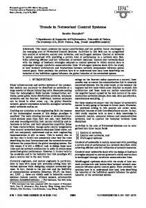
Figure 1. Model-Based Networked Control System

In [9] a model-based networked control system was introduced. The model-based networked control system architecture is shown in Figure 1. This control architecture has as main objective the reduction of the data packets transmitted over the network by a networked control system. To achieve this, the model-based networked control system uses knowledge of the plant. A model of the plant is used to predict the plant’s state vector dynamics and generate the appropriate control signal in between packet updates. In this way the amount of bandwidth necessitated by each control system using the network is minimized.

We will present different stability criteria that can be applied when the update times h(k) vary with time. The first case is when the statistical properties of h are unknown. The actual update times observed will jitter on the range [hmin, hmax]. This criterion may be used to provide a first cut on the stability properties of a system perhaps for comparison purposes. This is the strongest and most conservative stability criterion. This stability type is based on the classical Lyapunov function approach and thus will be referred to as Lyapunov Stability. Next we will present two stochastic stability criteria for systems in which the update times are independent, identically distributed random variables with probability distribution F(h). The first and strongest criterion is called Almost Sure Asymptotic Stability or Probability-1 Asymptotic Stability. This is the stochastic stability criterion that mostly resembles deterministic stability. The second and weaker type of stability is referred to as Mean Square Asymptotic Stability or Quadratic Asymptotic Stability.

The packets transmitted by the sensor contain the measured value of the plant state and are used to update the plant model on the actuator/controller node. These packets are transmitted at times tk. We define the update times as the times between transmissions or model updates: h(k)=tk+1-tk. In [9] we made the assumption that the update times h(k) are constant. This might not always be the case in applications. The transmission times of data packets from the plant output to the controller/actuator might not be completely periodic due to network contention and the usual nondeterministic nature of the transmitter task execution scheduler. Soft real time constraints provide a way to enforce the execution

0-7803-7896-2/03/$17.00 ©2003 IEEE

Finally a sufficient condition for Mean Square Stability for the model-based networked control system with update times following a finite state Markov chain is presented.

4119

Proceedings of the American Control Conference Denver, Colorado June 4-6, 2003


We focus our analysis on the Model-Based Networked Control System developed in [9], specifically the case where the plant is continuous and the states are available (full state feedback). Other networked systems (e.g. output feedback, discrete plants, etc) studied in [10,11] can be analyzed in a similar fashion.

matrix X such that Q = X − MXM T is positive definite for all

 I 0 Λh  I 0  e  . 0 0 0 0

h ∈ [hmin , hmax ] , where M = 

Proof. Noted that the output norm can be bounded by

2 Model-Based Networked Control System Response

 k  e Λ ( t − tk )  ∏ M ( j )  z0 ≤ e Λ ( t − tk ) ⋅  j =1 

The dynamics of the system shown in Figure 1 are given by:

− BK   x(t )   x(tk )   x(tk− )   x(t )   A + BK  , = e(t )  =   ;     A + BK Aˆ − BK  e(t )   e(tk )   0  (1) ∀t ∈ [tk , tk +1 ), with tk +1 − tk = h(k )

σ ( Λ ) hmax

≤e

z0 (3)

k

∏ M ( j) ⋅

z0

That is, since e Λ ( t − tk ) has a finite growth rate that will cease at most at hmax. Then convergence of the product of matrices M(j) to zero ensures the stability of the system.

representation, Aˆ and Bˆ are the matrices of plant model statespace representation, A = A − Aˆ and B = B − Bˆ represent the

It is clear that the range for h, that is the interval [hmin , hmax ] , will vary with the choice of X. Another observation is that the interval obtained this way will always be contained in the set of constant update times where the system is stable. That is, an update time contained in the interval [hmin , hmax ] will always be a stable constant update time.

modeling error matrices, and e(t ) = x(t ) − xˆ (t ) represents the error between the plant state and the plant model state. Define

 A + BK T e(t ) ] , and Λ =   A + BK

j =1

j =1

Where A and B are the matrices of actual plant state-space

now z (t ) = [ x(t )

⋅

k

∏ M ( j) ⋅

− BK   so Aˆ − BK 

that Equation (1) can be rewritten as z = Λz for t ∈ [tk , tk +1 ) . Proposition #1

4 Almost Sure Asymptotic Stability

The system described by Equation (1) with initial conditions

Now we assign to the update times some stochastic properties. We will assume that the update times h(j) are independent, identically distributed random variables. We now characterize the notion of stochastic stability. We will use the definition of almost sure asymptotic Lyapunov stability [6] that is the one that provides a stability criterion based on the sample path. Therefore, this stability definition resembles more the deterministic stability definition [7], and is of practical importance. It ensures that the system is asymptotically stable. The only weakness might be that the decaying rate may vary. But an expected decaying rate can still be specified. Since the stability condition has been relaxed, we expect to see less conservative results than those obtained using the Lyapunov stability previously considered. We now define Almost Sure or Probability-1 Asymptotic stability.

z (t0 ) = [ x(t0 ) 0] = z0 , has the following response: T

 k  z (t ) = e Λ (t −tk )  ∏ M ( j )  z0 ; t ∈ [tk , tk +1 ), tk +1 − tk = h(k ),  j =1    (2)  I 0  Λh ( j )  I 0  and M ( j ) =  e 0 0 . 0 0    The proof is similar to the one presented in [9] for constant update times and will be omitted here. We observe in Equation (2) that the response is given by a product of matrices that share the same structure but are in general different. Stability cannot be guaranteed even if all matrices in the product are stable or equivalently if they have their eigenvalues inside the unit circle. Next the stability criteria mentioned above are considered.

Definition #1 The equilibrium z = 0 of a system described by z = f (t , z ) with initial condition z (t0 ) = z0 is almost sure (or with probability-1) asymptotically stable at large (or globally) if for any β > 0 and

3 Lyapunov Stability

ε > 0 the solution of z = f ( t , z ) satisfies

This is the strongest and most conservative stability criterion. It is based on the well-known Lyapunov second method for determining the stability of a system. We will not consider the statistical properties of h(k). This criterion is not stochastic but provides a first approach to stability for cases in which the only thing that is known about the update times is that they are time varying and are contained within some interval.

  lim P sup z ( t , z0 , t0 ) > ε  = 0  t ≥δ 

δ →∞

(4)

Whenever z0 < β . This definition is similar to the one presented for deterministic systems. We will examine the conditions under which a full state feedback continuous networked system is stable. Let h=h(j) be independent identically distributed random sequence with probability distribution function F(h). We now present the

Theorem #1 The system described by Equation (2) is Lyapunov Stable for h ∈ [hmin , hmax ] if there exists a symmetric positive definite

4120



condition under which the system described by Equation (2) is asymptotically stable with probability 1.

1/ 2  h ( k * )   2  E  ∫ ξ k * (τ ) dτ    0     

Theorem #2 The system described by Equation (2), with update times h(j) independent identically distributed random variable with probability distribution F(h) is globally almost sure (or with probability-1) asymptotically stable around the solution

 h ( k * ) ≤ E  ∫ e Λτ   0

 x  0 z= =  e  0

 h ( k * ) ≤ E  ∫ eσ ( Λ )τ  0 

)

 h ( k * ) = E  ∫ eσ ( Λ )τ  0 

)

if

(

)

1/ 2 N = E  e 2σ ( Λ ) h − 1  < ∞  

and

0 Λh  I e  0 0

(

0 . 0

We will represent the system by using a technique similar to lifting [2] to obtain a discrete linear time invariant system. The system will be represented by

(

the operator Ω k as:

 E 

h(k )

(6)

 lim P sup ξ k (t0 , z0 ) δ →∞  k ≥δ

 >ε = 0 

2,[0,tk ]

z0 < β . It is obvious that the norm i

norm

 h( k )  2 =  ∫ ξ k (τ ) dτ     0 

bracketed

is

δ →∞

achieved

at

}

P sup ξ k > ε = P ξ k * > ε ≤ k ≥δ



j =1



∏ M ( j) 

z0

by

assumption

is

  = E  M  

(

)

k * −1

(10)

δ →∞

ε

(

) (

1/ 2 * 1   E  e 2σ ( Λ ) h ( k ) − 1  E  M  2σ (Λ)  

)

k * −1

(11)

z0

ε ~

[ ]

singular value E [σ M ] = E M < 1 . ♦

It is important to note that if this condition is applied directly over the test matrix M, we may end up with very conservative values. To correct this problem we can apply a similarity transformation over the test matrix M so to obtain a less conservative conclusion.

~ k * ≥ δ , that is

ε

k ≥δ

E  ξ k*   

identically zero (note that k * ≥ δ ) if the averaged maximum

is 2,[0, h ( k )]

. We will omit the

E  ξ k*   

}

It is obvious that the right hand side of the expression will be

An observation over the condition on the matrix N is that it ensures that the probability distribution function for the update times F(h) assigns smaller occurrence probabilities to increasingly long destabilizing update times. That is F(h) decays rapidly. In particular we observe that N can always be bounded if there exists hm such that F(h)=0 for h larger than hm. We can also bound the expression inside the expectation to obtain

k >δ

{

k * −1

δ →∞

(7)

positive random variables [13] to bound the probability in our definition:

}

k * −1

which

*   k −1 M ( j ) ≤ E   ∏ ∏ M ( j) j =1  j =1 

{

≤ lim

sup ξ k = ξ k * . So now we can use Chebyshev bound for

{

)

lim P sup ξ k > ε ≤ lim

subscript from now on. Now lets assume that the supremum of the

  E    

We can now evaluate the limit over the expression obtained.

1/ 2

2,[0, h ( k )]

 dτ   

(9)

k * −1

0

Now we can restructure the definition on almost sure stability or probability-1 stability given in Definition #1 to better fit the new system representation. We will say that the system represented by (5) is almost sure stable or stable with probability-1 if for any β > 0 and ε > 0 the solution of ξ k +1 = Ω k ξ k satisfies

given by ξ k

1/ 2

2

   

bounded. The second term can also be bounded by using the independency property of the update times h(j).

Here L2 e stands for the extended L2 . It is easy to obtain from (2)

whenever

z0

 dτ   

 M ( j ) z0  ∏  j =1 

1/ 2

 2 dτ   

1/ 2 * 1   E  e 2σ ( Λ ) h ( k ) − 1  2σ (Λ )  

ξ k +1 = Ω k ξ k , with ξ k ∈ L2 e and ξ k = z (t + tk ), t ∈ [0, hk ). (5)

∫ δ (τ − h(k ))ν (τ )dτ

∏ M ( j)

2

The last equation follows from the independency of the update times h(j). Analyzing the first term on the last equality we see that is bounded for the trival case where Λ = 0 . When Λ ≠ 0 , the integral can be solved, and can be showed to be equal to

Proof.

 I 0 (Ω kν )(t ) = eΛt   0 0

1/ 2

2

k * −1 j =1

(

the

expected value of the maximum singular value of the test matrix M, E  M  = E [σ M ] , is strictly less than one,

I where M =  0

2

(8)

(

)

E  e 2σ ( Λ ) h − 1 

Using (2) and basic norm properties, we proceed to bound the expectation on the right hand side

1/ 2

 < E eσ ( Λ ) h  and formulate the following   

corollary.

4121



Corollary #1

Definition #1

The system described by Equation (2), with update times h(j) that are independent identically distributed random variable with probability distribution F(h) is globally almost sure (or with probability-1) asymptotically stable around the solution

The equilibrium z = 0 of a system described by z = f (t , z ) with

z = [ x e] = [ 0 0] T

T

T = E  eσ ( Λ )h  < ∞

if

and

initial condition z (t0 ) = z0 is mean square stable asymptotically

stable at large (or globally) if the solution of z = f (t , z ) satisfies

the

expected value of the maximum singular value of the test matrix M, E M = E [σ M ] , is strictly less than one,

2 lim E  z ( t , z0 , t0 )  = 0  

[ ]

I 0

where M = 

0 Λh  I e  0 0

(12)

t →∞

0 . 0

A system that is mean square stable as defined previously will have the expectation of system states to be driven to zero with time. It is clear that this does not prevent the system states to be zero the whole time. For example, a system can have non-zero values at times that are separated in time by periods that increase with time can still satisfy the mean square stability condition since its average is converging to zero. So it is clear that this definition of stability is not as strong as probability-1 stability, but it is still attractive since many optimal control problems use the squared norm in their calculations. So we will present the conditions under which the networked control system described in (2) is mean square stable and how to these relate to the ones for probability-1 stability. Theorem #3

The system described by Equation (2), with update times h(j) independent identically distributed random variable with probability distribution F(h) is globally mean square

z = [ 0 0]

T

asymptotically stable around the solution

[ ]

(

for h~U(0.5,hmax) as a function of hmax.

E  M T M  = σ  E  M T M   , is        I 0 Λh  I 0 strictly less than one, where M =  e   . 0 0  0 0

Example use

)

 σ Λ h 2 K = E  e ( )  < ∞ and the maximum singular value of the  

Figure 2. Average Maximum Singular Value for σ M = E M

We

if

expected value of MTM,

an

unstable

plant,

the

double

integrator

0 1  0  where: A =  , B =   . For our plant model we chose: 0 0  1 0 0  ˆ  0  ˆ ˆ + Bu ˆ , xˆ = Ax Aˆ =   , B =   . Our feedback law is 0 0  0

Proof. Lets start by evaluating the expectation of the squared norm of the output of the system described by (2).

given by u=Kx with K = [ −1 −2] . We have seen in [9,10, 11]

  k  E  e Λ ( t − t k )  ∏ M ( j )  z0  j =1     

that the maximum constant update time h for which this system is stable is 1 second. We now assume a uniform probability distribution function U(0.5,hmax). The plot of averaged maximum singular value of a similarity transformation of the original test matrix M is shown in Figure 2. The similarity transformation used here was one that diagonalizes the matrix M for h=1.

 T = E  z0  

We see that the maximum value for hmax is around 1.3 seconds (maximum constant update time for stability is h=1 second.) So we see that, for example, a system with uniformly distributed update time from 0.5 to 1.2 seconds is stable, while a system with a constant update time of 1 second is unstable.

T

 k  ∏ M ( j)  j =1   

e Λ ( t − tk )

)

T

 k   e Λ ( t − t k )  ∏ M ( j )  z0   j =1     

)

e

 σ Λ h ( k +1) ≤ E e ( )  

)

 k  T z0  ∏ M ( j )   j =1   

(

We now present a weaker type of stability, namely Mean Square Asymptotic Stability that is defined next.

  

 ≤ E σ  eΛ (t −tk )   

(

5 Mean Square Asymptotic Stability

(

2

T

2

Λ ( t − tk )

z T  0 

T

 k  ∏ M ( j)  j =1    T

 k    ∏ M ( j )  z0     j =1  

 k    ∏ M ( j )  z0   j =1      (13)

4122



Now that the expectation is all in terms of the update times, we can use the independently identically distributed property of the update times and the assumption that K is bounded:

We now present a sufficient condition for the mean square stability of the system under markovian jumps. Theorem #4

 2  k   k   σ Λ h ( k +1) E e ( ) z0T  ∏ M ( j )   ∏ M ( j )  z0   j =1   j =1          T  k −1   k −1  T  = K ⋅ z0 E  ∏ M ( j )  M (k )T M (k )  ∏ M ( j )   z0   j =1   j =1     T  k −1   k −1  T  = K ⋅ z0 E  ∏ M ( j )  E  M T M   ∏ M ( j )   z0   j =1   j =1    

(

T

)

(

≤ K ⋅ σ E  M M  T

)

T z0 E

The system described by Equation (2), with update times h(k ) = hωk ≠ ∞ driven by a finite state Markov chain {ωk } with state space {1, 2,..., N } and transition probability matrix Γ with elements pi , j is globally mean square asymptotically stable around the solution z = [ x

(

( (

))

k

)

now

it

is

easy

to

see

T

z0 z0

that

 I 0 − z tk−+1 = e Λhk +1   z tk 0 0

( )

if

E  M T M  = σ  E  M T M   < 1 then the limit of the      

( )

Λhωk

(15)

 I 0   . Now 0 0 

we can represent the sampled networked control system as:

ς (k + 1) = H (ωk ) ς (k )

(16)

To ensure mean square stability we will make use of a Lyapunov function of quadratic form and analyze the expected value of its difference between two consecutive samples. We will use the following Lyapunov function:

V (ς (k ), ωk ) = ς (k )T P (ωk ) ς (k )

6 Mean Square Asymptotic Stability for Markovian Update Times

(17)

Now we can compute the expected value of the difference:

E [ ∆V | ς , i ]

Sometimes it is useful to represent the dynamics of the update times as driven by a Markov chain. A good example of this is when the network is susceptible to experience traffic congestion or has queues for message forwarding. We now present a stability criterion for the model-based control system in which the update times h(k) are driven by a finite state Markov chain. Assume that the update times can take a value from a finite set:

= E V (ς (k + 1), ωk +1 ) − V (ς (k ), ωk ) | ς (k ) = ς , ωk = i  = E ς (k + 1)T P ( ωk +1 ) ς (k + 1) | ς (k ) = ς , ωk = i  − ς T P ( i ) ς T = E ς T H (ωk ) P (ωk +1 ) H (ωk ) ς | ωk = i  − ς T P ( i ) ς  

(14)

N

(

)

= ∑ pi , j ς T H ( i ) P ( j ) H ( i ) ς − ς T P ( i ) ς

Lets represent the Markov chain process by {ωk } with state

j =1

T

 N  T = ς  ∑ pi , j H ( i ) P ( j ) H ( i ) − P ( i )  ς  j =1 

space {1, 2,..., N } and transition probability matrix Γ and NxN

T

matrix with elements pi , j . The transition probability matrix is

pi , j = Ρ{ωk +1 = j | ωk = i} .

and H ( ωk ) = e

−

The first thing we note is the similarity between the conditions given by Theorems #2 and #3. For the first and strongest one we require the expectation of the maximum singular value of the test matrix to be less than one. While for the second weaker stability it is required to have the maximum singular value of the expectation of MTM to be less than one.

defined as

( )

Lets define ς (k ) = z tk −1

expectation as time approaches infinity is zero, which concludes the proof.♦

h(k ) ∈ {h1 , h2 ,..., hN }

∀i, j = 1,..., N

We know that since the Markov chain has a finite number of states, and thus that the update times are bounded, we can analyze the system’s stability by sampling it at a certain time between each update time. We will evaluate the response of the system described by (2) at times tk− :

(11) So

if there exists

Proof.

We can repeat the last 3 steps recursively to finally obtain.

 ≤ K σ E M T M     

T

 N  T  ∑ pi , j H ( i ) P ( j ) H ( i ) − P ( i )  < 0  j =1  I 0   Λh with H ( i ) = e i  . 0 0 

T  k −1   k −1    ∏ M ( j )   ∏ M ( j )   z0   j =1   j =1    

2

T

positive definite matrices P(1), P(2), …, P(N) such that

(10)

  k  E  e Λ ( t − t k )  ∏ M ( j )  z0  j =1     

e] = [ 0 0]

So now we can

(

)

(18)

From this last equality is it obvious that to ensure mean square stability we need to have:

represent the update times more appropriately as h( k ) = hωk .

4123



 N  T  ∑ pi , j H ( i ) P ( j ) H ( i ) − P ( i )  < 0  j =1 

(

)

Proceedings Of The 40th IEEE Conference On Decision And Control, December 2001, pp. 191-196.

(19)♦

[6] F. Kozin, “A Survey of Stability of Stochastic Systems,” Automatica Vol5 pp. 95-112, 1968.

This type of stability criteria depend on our ability to find appropriate P(i) matrices. Several other results in jump system stability [1, 3] use a similar procedure that can be extended to obtain other conditions on stability of networked control systems. Note that most of the results available in the literature deal with similar but not identical type of systems. The relationship with Almost Sure stability can be studied by closely analyzing the implications of such simplification.

[7] M. Marion, “Jump Linear Systems in Automatic Control” Marcel Dekker, New York 1990. [8]A.S. Matveev, A.V. Savkin, “Optimal Control of Networked Systems via Asynchronous Communication Channels with Irregular Delays,” 40th IEEE Conference on Decision and Control, Orlando Florida, December 2001, pp. 2323-2332. [9] L.A. Montestruque, P.J. Antsaklis, “Model-Based Networked Control Systems: Necessary and Sufficient Conditions for Stability,” 10th Mediterranean Conference On Control And Automation, July 2002.

7 Conclusions In this paper four types of stability criteria for model-based networked control systems were presented. The first one ensures deterministic stability for an update time that can vary within an interval. The second stability criterion, called Almost Sure (or Probability-1) Stability, is a true stochastic stability criterion that ensures deterministic-like stability of a system. It assumes that the update times are independent identically distributed random variables. A weaker type of stochastic stability, Mean Square Stability, is also presented. It assumes independent identically distributed update times. Both stochastic stability criterion have similar structures and can be equivalent depending on the nature of the probability distribution function and the structure of the test matrix, as is the case for example when F(h)=0 for h>hm and the test matrix is diagonal. Finally, the case where the update time is governed by a Markov chain is studied and a sufficient condition for Mean Square Stability is derived.

[10] L.A. Montestruque, P.J. Antsaklis, “State And Output Feedback Control In Model-Based Networked Control Systems,” 41st IEEE Conference on Decision and Control, December 2002. [11] L.A. Montestruque and P.J. Antsaklis, “Model-Based Networked Control System - Stability,” ISIS Technical Report January 2001, ISIS-2002-001, http://www.nd.edu/~isis/techreports/isis-2002-001.pdf. [12] G. Walsh, H. Ye, and L. Bushnell, “Stability Analysis of Networked Control Systems,” Proceedings of American Control Conference, June 1999. [13] S. Woods, “Probability, Random Processes, and Estimation Theory for Engineers,” 2nd edition, Prentice Hall, Upper Saddle River 1994.

The stability types presented here only represent some of the different stochastic stability types available on the literature. We consider that the insight provided by the stability analysis studied here can be used to determine conditions for other stability types.

Acknowledgements The partial support of the DARPA/ITO-NEST Program (AFF30602-01-2-0526) is gratefully acknowledged.

References [1] O.L.V. Costa, M.D. Fragoso, “Stability Results for DiscreteTime Linear Systems with Markovian jumping Parameters,” Journal of Mathematical Analysis and Applications, Vol 179, pp. 154-178, 1993 [2] T. Chen, B. Francis, “Optimal Sampled-Data Control Systems,” 2nd edition, Springer, London 1996. [3]Y. Fang, “A New General Sufficient Condition for Almost Sure Stability of Jump Linear Systems,” IEEE Transactions on Automatic Control, Vol 42, No3, pp. 378-382, March 1997. [4] D. Hristu-Varsakelis, “Feedback Control Systems as Users of a Shared Network: Communication Sequences that Guarantee Stability,” Proceedings of the 40th IEEE Conference on Decision and Control, December 2001, pp. 3631-3636. [5] H. Ishii and B. Francis, “Stabilizing a Linear System by Switching Control and Output Feedback with Dwell Time,”

4124
