ABSTRACT. This paper presents computational approach for stock market prediction. Artificial Neural Network (ANN) forms a useful tool in predicting price ...
International Journal of Computer Applications (0975 – 8887) Volume 99– No.9, August 2014
Stock Market Prediction using Feed-forward Artificial Neural Network Suraiya Jabin Department of Computer Science, Jamia Millia Islamia, New Delhi
ABSTRACT This paper presents computational approach for stock market prediction. Artificial Neural Network (ANN) forms a useful tool in predicting price movement of a particular stock. In the short term, the pricing relationship between the elements of a sector holds firmly. An ANN can learn this pricing relationship to high degree of accuracy and be deployed to generate profits with sufficiently large amounts of data, preferably in times of low volatility and over a short time period. Experimental results are presented to demonstrate the performance of the proposed system. The paper also aims to suggest about training algorithms and training parameters that must be chosen in order to fit time series kind of complicated data to a neural network model. The proposed model succeeded in prediction of the trends of stock market with 100% prediction accuracy.
General Terms Pattern Recognition, Stock Market Prediction
Keywords BPNN, DAX, nntool, newff, trainbr, trainscg, trainrp
1. INTRODUCTION Prediction of stock market returns has been one of the most challenging problem to the AI community. For solving this problem, diverse kind of technical, fundamental, and statistical indicators have been proposed and used for example Regression, Support Vector Machines (SVM) with contrasting results. However, none of these techniques or combination of techniques had been successful enough. The objective of prediction research has been largely beyond the capability of traditional AI research which has mainly focused on developing intelligent systems that are supposed to emulate human intelligence. By its nature the stock market is mostly complex (non-linear) and volatile. With the development of artificial neural networks investors are benefitting by unleashing the market mysteries. These days’ artificial neural networks are considered as a common data mining method in different fields like economy, business, industry, weather forecasting and science. Artificial neural networks have been successfully used in stock market prediction during the last decade. The benchmark performance of neural network models in exchange rate forecasting has been established in a number of recent papers [1]. Neural network learning methods provide a robust approach to approximating real-valued, discrete valued, and vectorvalued target functions. The application of artificial neural networks in prediction problems is very promising due to some of their special characteristics. First, artificial neural networks can find the relationship between the input and output of the system even if this relationship might be very complicated because they are
general function approximations. Consequently, artificial neural networks are well applied to the problems in which extracting the relationships among data is really difficult but on the other hand there exists a large enough training data sets. Second, artificial neural networks have generalization ability meaning that after training they can recognize the new patterns even if they haven’t been in training set. Since in most of the pattern recognition problems predicting future events (unseen data) is based on previous data (training set), the application of artificial neural networks would be very beneficial. Third, artificial neural networks have been claimed to be excellent general function approximates. It is proved that a Multi-layer perceptrons (MLP) can approximate any complex continuous function that enables us to learn any complicated relationship between the input and the output of the system. Artificial neural networks are mostly used in predicting financial failures. This paper presents use of artificial neural networks to predict State Bank of India (SBI) Magnum Tax Gain scheme (Regular plan with growth option) Net Asset Value (NAV) value. The two year data set has been downloaded from bank’s website (www.sbimf.com). Multiple experiments were performed by taking different topologies of the feed forward network along with different training parameters like training function and transfer/output function. Experimental results are presented to demonstrate the performance of the error back propagation method for stock prediction.
2. REVIEW OF LITERATURE All ANNs are being used in various fields of application including business forecasting, credit scoring, bond rating, business failure prediction, medicine, pattern recognition, image processing, speech processing, computer vision and control systems. In the context of financial forecasting, Kuan and Liu [2] show that a properly designed ANN has lower out-of-sample mean squared prediction error relative to the random walk model. Jasic and Wood [3] discuss the profitability of trading signals generated from the out-ofsample short-term predictions for daily returns of S&P 500, DAX, TOPIX and FTSE stock market indices evaluated over the period 1965–99. The out-of sample prediction performance of neural networks is compared against a benchmark linear autoregressive model. They found that the buy and sell signals derived from neural network predictions are significantly different from unconditional one-day mean return and are likely to provide significant net profits for reasonable decision rules and transaction cost assumptions. They report that ANNs outperform the linear models from financial forecasting literature in terms of its predictive power. It is reported that the neural network models yield statistically lower forecast errors for the year-over year
4
International Journal of Computer Applications (0975 – 8887) Volume 99– No.9, August 2014 growth rate of real GDP relative to linear and univariate models. Huang et al. [4] report a comparative study of application of Support Vector Machines (SVM) and Backpropagation Neural Networks (BPNN) for an analysis of corporate credit ratings. They report that the performances of SVM and BNN in this problem were comparable and both these models achieved about 80 per cent prediction accuracy. It is reported that ANNs perform better than the statistical discriminant analysis both for training and hold-out samples. All the recent literatures [5, 6] have also echoed the same about neural networks.
3. BACK PROPAGATION METHOD Neural networks have been touted as all-powerful tools in stock-market prediction. Various companies claim amazing 199.2% returns over a 2-year period using their neural network prediction methods. Backpropagation neural network (BPNN) algorithm uses gradient descent to tune network parameters to best fit a training set of input-output pairs. BPNN has proven surprisingly successful in many practical problems such as learning to recognize hand written characters, to recognize spoken words and learning to recognize faces [7]. Backpropagation method combines Hill Climbing and Gradient Descent. It does Hill Climbing by Gradient Descent. Hill Climbing tries each possible step to choose a step that does the most good at every step. Gradient Descent tries moving in the direction of most rapid performance improvement. Gradient Descent requires a smooth threshold function and not the stair step threshold function which outputs 0 or 1 as stair step threshold function is discontinuous and is un-differentiable and hence unsuitable for gradient descent. One solution is the sigmoid unit, which is very much like a perceptron but based on a smoothed, differentiable threshold function. Athough in practice tansig (tan hyperbolic) function is preferred for faster learning. =1
.
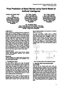
where D is the set of training examples, td is the target output for training example d, and od is the output of the linear unit for training example d. By this definition, E ( ) is simply half the squared difference between the target output td and thehear unit output od, summed over all training examples. Here we characterize E as a function of ( ), because the linear unit output o depends on this weight vector along with on a particular set of training examples. To understand the gradient descent algorithm it is helpful to visualize the entire hypothesis space of possible weight vectors and their associated error (E ( )) values, as illustrated in figure 2. This error surface is parabolic with a single global minimum for a single unit with just two inputs.
Fig 2: Error of different weight vectors for a linear unit with two weights Gradient descent search determines a weight vector that minimizes error E by starting with an arbitrary initial weight vector, then repeatedly modifying it in small steps. At each step, the weight vector is altered in the direction that produces the steepest descent along the error surface depicted in Figure 2. This process continues until the global minimum error is reached.
3.2 Backpropagation algorithm
. =
.
Fig 1: The Sigmoid Threshold Unit
3.1 Delta Training Rule The delta training rule is best understood by considering the task of training an unthresholded perceptron; that is, a linear unit for which the output O is given by:
Thus, a linear unit corresponds to the first stage of a perceptron, without the threshold. In order to derive a weight learning rule for linear units, let us begin by specifying a measure for the training error of a hypothesis (weight vector), relative to the training examples. Although there are many ways to define this error, one common measure that will turn out to be especially convenient is:
This algorithm learns the weights for a fully connected feedforward multilayer network. s. It employs gradient descent to attempt to minimize the squared error between the network output values and the target values for these outputs. Backpropagation (training_eaxamples, rate of learning ɳ, units in input layer nin, units in output layer nout, units in hidden layer nhidden) [7]: Each training example is a pair of the form ( , where is the vector of network input values, and is the vector of target network output values. The input from unit i into unit j is denoted xji, and the weight from unit i to unit j is denoted wji. a. Create a feed-forward network with nin, inputs, nhidden hidden units, and nout output units. b. Initialize all network weights to small random numbers (e.g., between -0.05 and +0.05). c. Until the termination condition is met, Do For each training eaxamples, do:
in
-Propagate the input forward through the network:
5
International Journal of Computer Applications (0975 – 8887) Volume 99– No.9, August 2014
Input the instance to the network and compute the output of every unit in the network.
-Propagate the errors backward through the network:
For each network output unit k, calculate its error term For each hidden unit h, calculate its error term
Update each network weight
One major difference in the case of multilayer networks is that the error surface can have multiple local minima, in contrast to the single minimum parabolic error surface shown in figure 2. Gradient descent is guaranteed only to converge toward some local minima, and not necessarily the global minimum error.
3.3 Convergence and local minima Despite the lack of assured convergence to the global minimum error, BPNN is a highly effective function approximation method in practice. In many practical applications the problem of local minima has not been found to be as severe as one might fear. To develop some intuition here, consider that networks with large numbers of weights correspond to error surfaces in very high dimensional spaces (one dimension per weight). When gradient descent falls into a local minimum with respect to one of these weights, it will not necessarily be in a local minimum with respect to the other weights. In fact, the more weights in the network, the more dimensions that might provide escape routes for gradient descent to fall away from the local minimum with respect to this single weight [7].
3.3.1 Accelerations to Backpropagation method A multilayer network, in general, learns much faster when the sigmoidal activation function is represented by a hyperbolic tangent (tanh). Also we can train multiple networks using the same data, but initializing each network with different random weights.
3.3.1.1 Use of momentum By making weight update on the nth iteration dependent on update during the (n-1) th iteration:
w ji (n) j x ji w ji (n 1)
here, 0 1, is a consant called momentum. traingdm is a network training function in MATLAB that updates weight and bias values according to gradient descent with momentum.
3.3.1.3 Adaptive learning rate If rate of learning is too large, the gradient descent search runs the risk of overstepping the minimum in the error surface rather than settling into it. To avoid it, common modification to the algorithm is to gradually reduce the value of learning rate as the no. of gradient descent steps grows. traingda is a network training function that updates weight and bias values according to gradient descent with adaptive learning rate. traingdx is a network training function in MATLAB that updates weight and bias values according to gradient descent momentum and an adaptive learning rate.
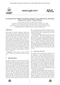
4. STOCK MARKET PREDICTION USING ANN 4.1 Data preprocessing A mutual fund (MF) is a financial product that pools money of different individuals and invest on their behalf into various assets such as equity, debt or gold. Based on one’s financial goal or risk appetite, there are several MF schemes to choose from. Few startling features that they offer are simplicity, affordability, professional management, diversification along with liquidity. The proposed work does prediction of Net Asset Value (NAV) of SBI mutual fund by training feedforward neural network. In stocks and businesses, NAV is an expression of the underlying value of the company; i.e. it is a statement of the value of the company's assets minus the value of its liabilities. One way of thinking about the net asset value is that it is the underlying value of a company, not the value dictated by the supply and demand of shares or its market capitalization. For the proposed work, the SBI magnum tax gain NAV values were taken for the duration of April 1, 2012 to April 4, 2014. Data is organized with regard to working days in Indian Stock Exchange. As a strategy, the sequences of 4 days’ index values were taken as input to predict each 5th day index value. In the training set 5th day’s NAV is the supervised value. The goal is to find such a weight matrix that minimizes the error at the output layer using backpropagation method. Next, the network topology is defined: what type of network, how many layers and how many neurons per layer are used. Actually, there is no rule for this, and usually it is determined experimentally. However the common type of network used for prediction is a multi layer perceptron. A recommendation is to have 2n+1 nodes for hidden-layer, where n is the number of the input nodes. The output layer has only one node in this case. The good results were obtained with the following topology and parameter set: maxIteration=10000, learningRate=0.7, maxerror=0.0001 also summarized in table 1 and table 2.
3.3.1.2 Use Incremental/ Stochastic gradient descent Stochastic gradient descent algorithm updates weights incrementally, upon examining each individual training example rather than computing weight updates after summing over the entire training example as was done in true gradient descent method. Here we have lesser computations. It can sometimes avoid falling into local minima as it uses the various gradients rather than just one gradient to guide its search.
6
International Journal of Computer Applications (0975 – 8887) Volume 99– No.9, August 2014 optimization. It minimizes a combination of squared errors and weights, and then determines the correct combination so as to produce a network that generalizes well. The process is called Bayesian regularization.
NAV at Day 1
NAV at Day 1
4.2.1.3 trainscg
Hidden unit 1 NAV at Day 5
NAV at Day 1
Hidden unit 2
NAV at Day 1 Input layer
Hidden layer
Output layer
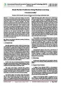
Fig 3: A simplified three-layer feed forward network to solve stock prediction on Day 5 when given input with previous four days values
4.2 Experiments Multiple experiments were performed by taking different topologies of the feed forward network along with different training parameters like training function and transfer/output function as summarized in table 1. Table 1. Parameters for creating network Training Function
Adaption Learning Function
trainrp
learngdm
trainbr
learngdm
trainscg
learngdm
Performance Function MSE (Mean Squared Error) SSE (Sum Squared Error) SSE (Mean Squared Error)
trainscg is a network training function that updates weight and bias values according to the scaled conjugate gradient method.
4.3 Results and Discussion The process of training a neural network involves tuning the values of weights and biases of the network to optimize network performance function. The default performance function for feed-forward network is mean square error (mse) i.e. the average squared error between the network outputs and the target outputs. Experimental results are presented to demonstrate the performance of the backpropagation method for stock prediction.Training occurs according to following training parameters, shown in table 2 with their experimental and default values. Table 2. The chosen training parameters Parameter
net.trainParam.epochs
Experimental Vaule 10000
net.trainParam.goal
0
Transfer Function
net.trainParam.max_fail
600
4-2020-201
Tansig /logsig
net.trainParam.min_grad
1e-7
4-2020-201
Tansig/ logsig
net.trainParam.mu
0.001
4-2020-201
Tansig/ logsig
net.trainParam.mu_dec net.trainParam.mu_inc net.trainParam.mu_max net.trainParam.show
0.1 10 1e10 25
net.trainParam.showCom mandLine net.trainParam.showWin dow net.trainParam.time
0
Topology
4.2.1 Training functions The default training function is trainlm but it could not do well for stock prediction. When training large networks and specially training for pattern recognition, trainbr, trainscg and trainrp are good choices. For training the feed forward network, different training functions were tried with different topologies of the network (e.g. 4-20-20-20-1, 4-20-20-1, 4-1515-1, 4-20-1, 4-40-1) and after exhaustive experiments with varying training functions, it was found that with following three training functions, good results can be obtained for learning time-series kind of data.
4.2.1.1 trainrp trainrp is a network training function that updates weight and bias values according to the resilient backpropagation algorithm (Rprop).
4.2.1.2 trainbr trainbr is a network training function that updates the weight and bias values according to Levenberg-Marquardt
1 Inf
Description with default value Maximum number of epochs to train; default value 1000 Performance goal (to minimize error) Maximum validation failures; default value=6 Minimum performance gradient Initial mu (the learning rate) mu decrease factor mu increase factor Maximum mu Epochs between displays (NaN for no displays) Generate commandline output Show training GUI Maximum time to train in seconds
Training stops when any of these conditions occurs [8]:
The maximum number of epochs (repetitions) is reached. The maximum amount of time is exceeded. Performance is minimized to the goal. The performance gradient falls below min_grad. mu exceeds mu_max. Validation performance has increased more than max_fail times since the last time it decreased (when using validation).
7
International Journal of Computer Applications (0975 – 8887) Volume 99– No.9, August 2014 The experimental results are summarized in table 3. It is found that the results were not satisfactory for networks with just one hidden layer. The training function trainbr performed well for 2 or 3 hidden layers. Table 3. Results of two most successful experiments with Feed-forward backpropagation network with best results from training function trainbr Topology
Training Function
Best Validation Performance
Regression Train -ing
Vali dati on
Test
4-20trainbr 0.13104 at 1 1 1 20-20-1 epoch 691 4-20trainbr 0.22893 at 1 0.89 0.95 20-1 epoch 3061 Experiments suggested that trainbr is the most suitable training method for stock market prediction.
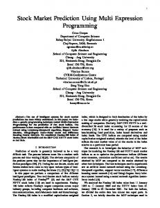
5. ANALYSIS OF NETWORK AFTER TRAINING The figure 4 shows the plot of validation performance versus each iteration for proposed feed-forward network model with topology 4-20-20-20-1 and trainbr as the training function chosen. Training stops when the performance on the nontraining validation set fails to decrease. The next step in validating the network is to create a regression plot, which shows the relationship between the outputs of the network and the targets. If the training were perfect, the network outputs and the targets would be exactly equal, but the relationship is rarely perfect in practice.
variations in no. of hidden layers, no. of neurons in hidden layers, and different training parameters. Larger numbers of neurons in the hidden layer give the network more flexibility because the network has more parameters it can optimize but at the same time it increases time and space complexity. Experiments were done by increasing the layer size gradually. If hidden layer size is made too large, it may cause the problem to be under-characterized and it may result in the network optimizing more parameters than there are data vectors to constrain these parameters. While experimenting with different training functions it was found that Bayesian regularization training with trainbr produces better generalization capability than using early stopping. The following conclusion can be drawn about ANNs; it has ability to extract useful information from large set of data therefore ANNs play very important role in stock market prediction.
7. ACKNOWLEDGMENTS My special thanks to the students (Deepak Bisht and Rajesh Maulekhi) who contributed towards preprocessing of the data set.
8. REFERENCES [1] Teo Jasic, Douglas Wood: Neural network protocols and model performance. Neurocomputing 55(3-4): 747-753 (2003) [2] Chung-Ming Kuan and Tung Liu. December (1995). Forecasting Exchange Rates Using Feedforward and Recurrent Neural Networks. Journal of Applied of Econometrics 10 (4): 347-364. [3] Mn Y. LeCun, L. D. Jackel, B. Boser, J. S. Denker, H. P. Graf, I. Guyon, D. Henderson, R. E. Howard and W. Hubbard: Handwritten Digit Recognition: Applications of Neural Net Chips and Automatic Learning, IEEE Communication, 41-46, invited paper, November 1989. [4] Min, J. H., & Lee, Y. C. (2005). Bankruptcy prediction using support vector machine with optimal choice of kernel function parameters. Expert systems with applications, 28(4), 603-614. [5] Najeb Masoud, Predicting Direction of Stock Prices Index Movement Using Artificial Neural Networks:The Case of Libyan Financial Market, British Journal of Economics, Management & Trade, 4(4): 597-619, 2014. [6] Akbilgic, O., Bozdogan, H., Balaban, M.E., (2013) A novel Hybrid RBF Neural Networks model as a forecaster, Statistics and Computing. DOI 10.1007/s11222-013-9375-7
Fig 4: Performance plot of feed-forward network with topology 4-20-20-20-1 and training function trainbr
[7] Mitchell, Tom M. "Machine learning. 1997." Burr Ridge, IL: McGraw Hill 45 (1997).
6. CONCLUSIONS This paper investigates stock market prediction using feedforward neural network. Experiments were done by doing
IJCATM : www.ijcaonline.org
8