Strabon: A Semantic Geospatial DBMS ⋆. Kostis Kyzirakos, Manos
Karpathiotakis, and Manolis Koubarakis. National and Kapodistrian University of
Athens, ...
Strabon: A Semantic Geospatial DBMS
?
Kostis Kyzirakos, Manos Karpathiotakis, and Manolis Koubarakis National and Kapodistrian University of Athens, Greece {kkyzir,mk,koubarak}@di.uoa.gr
Abstract. We present Strabon, a new RDF store that supports the state of the art semantic geospatial query languages stSPARQL and GeoSPARQL. To illustrate the expressive power offered by these query languages and their implementation in Strabon, we concentrate on the new version of the data model stRDF and the query language stSPARQL that we have developed ourselves. Like GeoSPARQL, these new versions use OGC standards to represent geometries where the original versions used linear constraints. We study the performance of Strabon experimentally and show that it scales to very large data volumes and performs, most of the times, better than all other geospatial RDF stores it has been compared with.
1
Introduction
The Web of data has recently started being populated with geospatial data. A representative example of this trend is project LinkedGeoData where OpenStreetMap data is made available as RDF and queried using the declarative query language SPARQL. Using the same technologies, Ordnance Survey makes available various geospatial datasets from the United Kingdom. The availability of geospatial data in the linked data “cloud” has motivated research on geospatial extensions of SPARQL [7, 9, 13]. These works have formed the basis for GeoSPARQL, a proposal for an Open Geospatial Consortium (OGC) standard which is currently at the “candidate standard” stage [1]. In addition, a number of papers have explored implementation issues for such languages [2, 3]. In this paper we present our recent achievements in both of these research directions and make the following technical contributions. We describe a new version of the data model stRDF and the query language stSPARQL, originally presented in [9], for representing and querying geospatial data that change over time. In the new version of stRDF, we use the widely adopted OGC standards Well Known Text (WKT) and Geography Markup Language (GML) to represent geospatial data as literals of datatype strdf:geometry (Section 2). The new version of stSPARQL is an extension of SPARQL 1.1 which, among other features, offers functions from the OGC standard “OpenGIS Simple Feature Access for SQL” for the manipulation of spatial ?
This work was supported in part by the European Commission project TELEIOS (http://www.earthobservatory.eu/)
literals and support for multiple coordinate reference systems (Section 3). The new version of stSPARQL and GeoSPARQL have been developed independently at about the same time. We discuss in detail their many similarities and few differences and compare their expressive power. We present the system Strabon1 , an open-source semantic geospatial DBMS that can be used to store linked geospatial data expressed in stRDF and query them using stSPARQL. Strabon can also store data expressed in RDF using the vocabularies and encodings proposed by GeoSPARQL and query this data using the subset of GeoSPARQL that is closer to stSPARQL (the union of the GeoSPARQL core, the geometry extension and the geometry topology extension [1]). Strabon extends the RDF store Sesame, allowing it to manage both thematic and spatial RDF data stored in PostGIS. In this way, Strabon exposes a variety of features similar to those offered by geospatial DBMS that make it one of the richest RDF store with geospatial support available today. Finally, we perform an extensive evaluation of Strabon using large data volumes. We use a real-world workload based on available geospatial linked datasets and a workload based on a synthetic dataset. Strabon can scale up to 500 million triples and answer complex stSPARQL queries involving the whole range of constructs offered by the language. We present our findings in Section 5, including a comparison between Strabon on top of PostgreSQL and a proprietary DBMS, the implementation presented in [3], the system Parliament [2], and a baseline implementation. Thus, we are the first to provide a systematic evaluation of RDF stores supporting languages like stSPARQL and GeoSPARQL and pointing out directions for future research in this area.
2
A new version of stRDF
In this section we present a new version of the data model stRDF that was initially presented in [9]. The presentation of the new versions of stRDF and stSPARQL (Section 3) is brief since the new versions are based on the initial ones published in [9]. In [9] we followed the ideas of constraint databases [12] and chose to represent spatial and temporal data as quantifier-free formulas in the first-order logic of linear constraints. These formulas define subsets of Qk called semi-linear point sets in the constraint database literature. In the original version of stRDF, we introduced the data type strdf:SemiLinearPointSet for modeling geometries. The values of this datatype are typed literals (called spatial literals) that encode geometries using Boolean combinations of linear constraints in Q2 . For example, (x ≥ 0 ∧ y ≥ 0 ∧ x + y ≤ 1) ∨ (x ≤ 0 ∧ y ≤ 0 ∧ x + y ≥ −1) is such a literal encoding the union of two polygons in Q2 . In [9] we also allow the representation of valid times of triples using the proposal of [6]. Valid times are again represented using order constraints over the time structure Q. In the rest of this paper we omit the temporal dimension of stRDF from our discussion and concentrate on the geospatial dimension only. 1
http://www.strabon.di.uoa.gr
Although our original approach in [9] results in a theoretically elegant framework, none of the application domains we worked with had geospatial data represented using constraints. Today’s GIS practitioners represent geospatial data using OGC standards such as WKT and GML. Thus, in the new version of stRDF and stSPARQL, which has been used in EU projects SemsorGrid4Env and TELEIOS, the linear constraint representation of spatial data was dropped in favour of OGC standards. As we demonstrate below, introducing OGC standards in stRDF and stSPARQL has been achieved easily without changing anything from the basic design choices of the data model and the query language. In the new version of stRDF, the datatypes strdf:WKT and strdf:GML are introduced to represent geometries serialized using the OGC standards WKT and GML. WKT is a widely accepted OGC standard2 and can be used for representing geometries, coordinate reference systems and transformations between coordinate reference systems. A coordinate system is a set of mathematical rules for specifying how coordinates are to be assigned to points. A coordinate reference system (CRS) is a coordinate system that is related to an object (e.g., the Earth, a planar projection of the Earth) through a so-called datum which specifies its origin, scale, and orientation. Geometries in WKT are restricted to 0-, 1- and 2-dimensional geometries that exist in R2 , R3 or R4 . Geometries that exist in R2 consist of points with coordinates x and y, e.g., POINT(1,2). Geometries that exist in R3 consist of points with coordinates x, y and z or x, y and m where m is a measurement. Geometries that exist in R4 consist of points with coordinates x, y, z and m. The WKT specification defines syntax for representing the following classes of geometries: points, line segments, polygons, triangles, triangulated irregular networks and collections of points, line segments and polygons. The interpretation of the coordinates of a geometry depends on the CRS that is associated with it. GML is an OGC standard3 that defines an XML grammar for modeling, exchanging and storing geographic information such as coordinate reference systems, geometries and units of measurement. The GML Simple Features specification (GML-SF) is a profile of GML that deals only with a subset of GML and describes geometries similar to the one defined by WKT. Given the OGC specification for WKT, the datatype strdf:WKT4 is defined as follows. The lexical space of this datatype includes finite-length sequences of characters that can be produced from the WKT grammar defined in the WKT specification, optionally followed by a semicolon and a URI that identifies the corresponding CRS. The default case is considered to be the WGS84 coordinate reference system. The value space is the set of geometry values defined in the WKT specification. These values are a subset of the union of the powersets of R2 and R3 . The lexical and value space for strdf:GML are defined similarly. The datatype strdf:geometry is also introduced to represent the serialization of a geometry independently of the serialization standard used. The datatype 2 3 4
http://portal.opengeospatial.org/files/?artifact_id=25355 http://portal.opengeospatial.org/files/?artifact_id=39853 http://strdf.di.uoa.gr/ontology
strdf:geometry is the union of the datatypes strdf:WKT and strdf:GML, and appropriate relationships hold for its lexical and value spaces. Both the original [9] and the new version of stRDF presented in this paper impose minimal new requirements to Semantic Web developers that want to represent spatial objects with stRDF; all they have to do is utilize a new literal datatype. These datatypes (strdf:WKT, strdf:GML and strdf:geometry) can be used in the definition of geospatial ontologies needed in applications, e.g., ontologies similar to the ones defined in [13]. In the examples of this paper we present stRDF triples that come from a fire monitoring and burnt area mapping application of project TELEIOS. The prefix noa used refers to the namespace of relevant vocabulary5 defined by the National Observatory of Athens (NOA) for this application. Example 1. stRDF triples derived from GeoNames that represent information about the Greek town Olympia including an approximation of its geometry. Also, stRDF triples that represent burnt areas. geonames:26 rdf:type dbpedia:Town. geonames:26 geonames:name "Olympia". geonames:26 strdf:hasGeometry "POLYGON((21 18,23 18,23 21,21 21,21 18)); "^^strdf:WKT. noa:BA1 rdf:type noa:BurntArea; strdf:hasGeometry "POLYGON((0 0,0 2,2 2,2 0,0 0))"^^strdf:WKT. noa:BA2 rdf:type noa:BurntArea; strdf:hasGeometry "POLYGON((3 8,4 9,3 9,3 8))"^^strdf:WKT.
Features can, in general, have many geometries (e.g., for representing the feature at different scales). Domain modelers are responsible for their appropriate utilization in their graphs and queries.
3
A new version of stSPARQL
In this section we present a new version of the query language stSPARQL that we originally introduced in [9]. The new version is an extension of SPARQL 1.1 with functions that take as arguments spatial terms and can be used in the SELECT, FILTER, and HAVING clause of a SPARQL 1.1 query. A spatial term is either a spatial literal (i.e., a typed literal with datatype strdf:geometry or its subtypes), a query variable that can be bound to a spatial literal, the result of a set operation on spatial literals (e.g., union), or the result of a geometric operation on spatial terms (e.g., buffer). In stSPARQL we use functions from the “OpenGIS Simple Feature Access - Part 2: SQL Option” standard (OGC-SFA)6 for querying stRDF data. This standard defines relational schemata that support the storage, retrieval, query and update of sets of simple features using SQL. A feature is a domain entity that can have various attributes that describe spatial and non-spatial (thematic) characteristics. The spatial characteristics of 5 6
http://www.earthobservatory.eu/ontologies/noaOntology.owl http://portal.opengeospatial.org/files/?artifact_id=25354
a feature are represented using geometries such as points, lines, polygons, etc. Each geometry is associated with a CRS. A simple feature is a feature with all spatial attributes described piecewise by a straight line or a planar interpolation between sets of points. The OGC-SFA standard defines functions for requesting a specific representation of a geometry (e.g., the function ST_AsText returns the WKT representation of a geometry), functions for checking whether some condition holds for a geometry (e.g., the function ST_IsEmpty returns true if a geometry is empty) and functions for returning some properties of the geometry (e.g., the function ST_Dimension returns its inherent dimension). In addition, the standard defines functions for testing named spatial relationships between two geometries (e.g., the function ST_Overlaps) and functions for constructing new geometries from existing geometries (e.g., the function ST_Envelope that returns the minimum bounding box of a geometry). The new version of stSPARQL extends SPARQL 1.1 with the machinery of the OGC-SFA standard. We achieve this by defining a URI for each of the SQL functions defined in the standard and use them in SPARQL queries. For example, for the function ST IsEmpty defined in the OGC-SFA standard, we introduce the SPARQL extension function xsd:boolean strdf:isEmpty(strdf:geometry g) which takes as argument a spatial term g, and returns true if g is the empty geometry. Similarly, we have defined a Boolean SPARQL extension function for each topological relation defined in OGC-SFA (topological relations for simple features), [5] (Egenhofer relations) and [4] (RCC-8 relations). In this way stSPARQL supports multiple families of topological relations our users might be familiar with. Using these functions stSPARQL can express spatial selections, i.e., queries with a FILTER function with arguments a variable and a constant (e.g., strdf:contains(?geo, "POINT(1 2)"^^strdf:WKT)), and spatial joins, i.e., queries with a FILTER function with arguments two variables (e.g., strdf:contains(?geoA, ?geoB)). The stSPARQL extension functions can also be used in the SELECT clause of a SPARQL query. As a result, new spatial literals can be generated on the fly during query time based on pre-existing spatial literals. For example, to obtain the buffer of a spatial literal that is bound to the variable ?geo, we would use the expression SELECT (strdf:buffer(?geo,0.01) AS ?geobuffer). In stSPARQL we have also the following three spatial aggregate functions: – strdf:geometry strdf:union(set of strdf:geometry a), returns a geometry that is the union of the set of input geometries. – strdf:geometry strdf:intersection(set of strdf:geometry a), returns a geometry that is the intersection of the set of input geometries. – strdf:geometry strdf:extent(set of strdf:geometry a), returns a geometry that is the minimum bounding box of the set of input geometries. stSPARQL also supports update operations (insertion, deletion, and update of stRDF triples) conforming to the declarative update language for SPARQL, SPARQL Update 1.1, which is a current proposal of W3C. The following examples demonstrate the functionality of stSPARQL.
Example 2. Return the names of towns that have been affected by fires. SELECT ?name WHERE { ?t a dbpedia:Town; geonames:name ?name; strdf:hasGeometry ?tGeo. ?ba a noa:BurntArea; strdf:hasGeometry ?baGeo. FILTER(strdf:intersects(?tGeo,?baGeo))}
The query above demonstrates how to use a topological function in a query. The results of this query are the names of the towns whose geometries “spatially overlap” the geometries corresponding to areas that have been burnt. Example 3. Isolate the parts of the burnt areas that lie in coniferous forests. SELECT ?ba (strdf:intersection(?baGeom,strdf:union(?fGeom)) AS ?burnt) WHERE { ?ba a noa:BurntArea. ?ba strdf:hasGeometry ?baGeom. ?f a noa:Area. ?f noa:hasLandCover noa:ConiferousForest. ?f strdf:hasGeometry ?fGeom. FILTER(strdf:intersects(?baGeom,?fGeom)) } GROUP BY ?ba ?baGeom
The query above tests whether a burnt area intersects with a coniferous forest. If this is the case, groupings are made depending on the burnt area. The geometries of the forests corresponding to each burnt area are unioned, and their intersection with the burnt area is calculated and returned to the user. Note that only strdf:union is an aggregate function in the SELECT clause; strdf:intersection performs a computation involving the result of the aggregation and the value of ?baGeom which is one of the variables determining the grouping according to which the aggregate computation is performed. More details of stRDF and stSPARQL are given in [11].
4
Implementation
Strabon 3.0 is a fully-implemented, open-source, storage and query evaluation system for stRDF/stSPARQL and the corresponding subset of GeoSPARQL. We concentrate on stSPARQL only, but given the similarities with GeoSPARQL to be discussed in Section 6, the applicability to GeoSPARQL is immediate. Strabon has been implemented by extending the widely-known RDF store Sesame. We chose Sesame because of its open-source nature, layered architecture, wide range of functionalities and the ability to have PostGIS, a ‘spatially enabled’ DBMS, as a backend to exploit its variety of spatial functions and operators. Strabon is implemented by creating a layer that is included in Sesame’s software stack in a transparent way so that it does not affect its range of functionalities, while benefitting from new versions of Sesame. Strabon 3.0 uses Sesame 2.6.3 and comprises three modules: the storage manager, the query engine and PostGIS. The storage manager utilizes a bulk loader to store stRDF triples using the “one table per predicate” scheme of Sesame and dictionary encoding. For each predicate table, two B+ tree two-column indices are created. For each dictionary table a B+ tree index on the id column is created. All spatial literals are
also stored in a table with schema geo values(id int, value geometry, srid int). Each tuple in the geo values table has an id that is the unique encoding of the spatial literal based on the mapping dictionary. The attribute value is a spatial column whose data type is the PostGIS type geometry and is used to store the geometry that is described by the spatial literal. The geometry is transformed to a uniform, user-defined CRS and the original CRS is stored in the attribute srid. Additionally, a B+ tree index on the id column and an R-tree-over-GiST spatial index on the value column are created. Query processing in Strabon is performed by the query engine which consists of a parser, an optimizer, an evaluator and a transaction manager. The parser and the transaction manager are identical to the ones in Sesame. The optimizer and the evaluator have been implemented by modifying the corresponding components of Sesame as we describe below. The query engine works as follows. First, the parser generates an abstract syntax tree. Then, this tree is mapped to the internal algebra of Sesame, resulting in a query tree. The query tree is then processed by the optimizer that progressively modifies it, implementing the various optimization techniques of Strabon. Afterwards, the query tree is passed to the evaluator to produce the corresponding SQL query that will be evaluated by PostgreSQL. After the SQL query has been posed, the evaluator receives the results and performs any postprocessing actions needed. The final step involves formatting the results. Besides the standard formats offered by RDF stores, Strabon offers KML and GeoJSON encodings, which are widely used in the mapping industry. We now discuss how the optimizer works. First, it applies all the Sesame optimizations that deal with the standard SPARQL part of an stSPARQL query (e.g., it pushes down FILTERs to minimize intermediate results etc.). Then, two optimizations specific to stSPARQL are applied. The first optimization has to do with the extension functions of stSPARQL. By default, Sesame evaluates these after all bindings for the variables present in the query are retrieved. In Strabon, we modify the behaviour of the Sesame optimizer to incorporate all extension functions present in the SELECT and FILTER clause of an stSPARQL query into the query tree prior to its transformation to SQL. In this way, these extension functions will be evaluated using PostGIS spatial functions instead of relying on external libraries that would add an unneeded post-processing cost. The second optimization makes the underlying DBMS aware of the existence of spatial joins in stSPARQL queries so that they would be evaluated efficiently. Let us consider the query of Example 2. The first three triple patterns of the query are related to the rest via the topological function strdf:intersects. The query tree that is produced by the Sesame optimizer, fails to deal with this spatial join appropriately. It will generate a Cartesian product for the third and the fifth triple pattern of the query, and the evaluation of the spatial predicate strdf:intersects will be wrongly postponed after the calculation of this Cartesian product. Using a query graph as an intermediate representation of the query, we identify such spatial joins and modify the query tree with appropriate nodes so that Cartesian products are avoided. For the query of Example 2, the
modified query tree will result in a SQL query that contains a θ-join where θ is the spatial function ST Intersects. More details of the query engine including examples of query trees and the SQL queries produced are given in the long version of this paper7 . To quantify the gains of the optimization techniques used in Strabon, we also developed a naive, baseline implementation of stSPARQL which has none of the optimization enhancements to Sesame discussed above. The naive implementation uses the native store of Sesame as a backend instead of PostGIS (since the native store outperforms all other Sesame implementations using a DBMS). Data is stored on disk using atomic operations and indexed using B-Trees.
5
Experimental Evaluation
This section presents a detailed evaluation of the system Strabon using two different workloads: a workload based on linked data and a synthetic workload. For both workloads, we compare the response time of Strabon on top of PostgreSQL (called Strabon PG from now on) with our closest competitor implementation in [3], the naive, baseline implementation described in Section 4, and the RDF store Parliament. To identify potential benefits from using a different DBMS as a relational backend for Strabon, we also executed the SQL queries produced by Strabon in a proprietary spatially-enabled DBMS (which we will call System X, and Strabon X the resulting combination). [3] presents an implementation which enhances the RDF-3X triple store with the ability to perform spatial selections using an R-tree index. The implementation of [3] is not a complete system like Strabon and does not support a full-fledged query language such as stSPARQL. In addition, the only way to load data in the system is the use of a generator which has been especially designed for the experiments of [3] thus it cannot be used to load other datasets in the implementation. Moreover, the geospatial indexing support of this implementation is limited to spatial selections. Spatial selections are pushed down in the query tree (i.e., they are evaluated before other operators). Parliament is an RDF storage engine recently enhanced with GeoSPARQL processing capabilities [2], which is coupled with Jena to provide a complete RDF system. Our experiments were carried out on an Ubuntu 11.04 installation on an Intel Xeon E5620 with 12MB L2 cache running at 2.4 GHz. The system has 16GB of RAM and 2 disks of striped RAID (level 0). We measured the response time for each query posed by measuring the elapsed time from query submission till a complete iteration over the results had been completed. We ran all queries five times on cold and warm caches. For warm caches, we ran each query once before measuring the response time, in order to warm up the caches. 7
http://www.strabon.di.uoa.gr/files/Strabon-ISWC-2012-long-version.pdf
Dataset
Size
Triples
Spatial terms
Distinct spatial terms
Points
DBpedia GeoNames LGD
7.1 GB 2.1GB 6.6GB
58,727,893 17,688,602 46,296,978
386,205 1,262,356 5,414,032
375,087 1,099,964 5,035,981
375,087 1,099,964 3,205,015
Linestrings (min/ max/ avg # of points/ linestring) 353,714 (4/20/9)
Pachube SwissEx CLC
828KB 33MB 14GB
6,333 277,919 19,711,926
101 687 2,190,214
70 623 2,190,214
70 623 -
-
GADM
146MB
255
51
51
-
-
Polygons (min/max/avg # of points/ polygon) 1,704,650 (4/20/9) 2,190,214 (4/1,255,917/129) 51 (96/ 510,018/ 79,831)
Fig. 1: Summary of unified linked datasets
5.1
Evaluation using Linked Data
This section describes the experiments we did to evaluate Strabon using a workload based on linked data. We combined multiple popular datasets that include geospatial information: DBpedia, GeoNames, LinkedGeoData, Pachube, Swiss Experiment. We also used the datasets Corine Land Use/Land Cover and Global Administrative Areas that were published in RDF by us in the context of the EU projects TELEIOS and SemsorGrid4Env. The size of the unified dataset is 30GB and consists of 137 million triples that include 176 million distinct RDF terms, of which 9 million are spatial literals. As we can see in Table 1, the complexity of the spatial literals varies significantly. More information on the datasets mentioned and the process followed can be found in the long version of the paper. It should be noted that we could not use the implementation of [3] to execute this workload since it is not a complete system like Strabon as we explained above. Storing stRDF Documents. For our experimental evaluation, we used the bulk loader mentioned in Section 4 emulating the “per-predicate” scheme since preliminary experiments indicated that the query response times in PostgreSQL were significantly faster when using this scheme compared to the “monolithic” scheme. This decision led to the creation of 48,405 predicate tables. Figure 2a presents the time required by each system to store the unified dataset. The difference in times between Strabon and the naive implementation is natural given the very large number of predicate tables that had to be produced, processed and indexed. In this dataset, 80% of the total triples used only 17 distinct predicates. The overhead imposed to process the rest 48,388 predicates cancels the benefits of the bulk loader. A hybrid solution storing triples with popular predicates in separate tables while storing the rest triples in a single table, would have been more appropriate for balancing the tradeoff between storage time and query response time but we have not experimented with this option. In Section 5.2 we show that the loader scales much better when fewer distinct predicates are present in our dataset, regardless its size. In the case of Strabon X, we followed the same process with Strabon PG. System X required double the amount of time that it took PostgreSQL to store and index the data. In the case of Parliament we modified the dataset to conform
to GeoSPARQL and measured the time required for storing the resulting file. After incorporating the additional triples required by GeoSPARQL, the resulting dataset had approximately 15% more triples than the original RDF file. Evaluating stSPARQL Queries. In this experiment we chose to evaluate Strabon using eight real-world queries. Our intention was to have enough queries to demonstrate Strabon’s performance and functionality based on the following criteria: query patterns should be frequently used in Semantic Web applications or demonstrate the spatial extensions of Strabon. The first criterion was fulfilled by taking into account the results of [14] when designing the queries. [14] presents statistics on real-world SPARQL queries based on the logs of DBpedia. We also studied the query logs of the LinkedGeoData endpoint (which were kindly provided to us) to determine what kind of spatial queries are popular. According to this criterion, we composed the queries Q1, Q2 and Q7. According to [14] queries like Q1 and Q2 that consist of a few triple patterns are very common. Query Q7 consists of few triple patterns and a topological FILTER function, a structure similar to the queries most frequently posed to the LGD endpoint. The second criterion was fulfilled by incorporating spatial selections (Q4 and Q5) and spatial joins (Q3,Q6,Q7 and Q8) in the queries. In addition, we used nontopological functions that create new geometries from existing ones (Q4 and Q8) since these functions are frequently used in geospatial relational databases. In Table 2b we report the response time results. In queries Q1 and Q2, the baseline implementation outperforms all other systems as these queries do not include any spatial function. As mentioned earlier, the native store of Sesame outperforms Sesame implementations on top of a DBMS. All other systems produce comparable result times for these non-spatial queries. In all other queries the DBMS-based implementations outperform Parliament and the naive implementation. Strabon PG outperforms the naive implementation since it incorporates the two stSPARQL-specific optimizations discussed in Section 4. Thus, spatial operations are evaluated by PostGIS using a spatial index, instead of being evaluated after all the results have been retrieved. The naive implementation and Parliament fail to execute Q3 as this query involves a spatial join that is very expensive for systems using a naive approach. The only exception in the behavior of the naive implementation is Q4 in the case of warm caches, where the nonspatial part of the query produces very few results and the file blocks needed for query evaluation are cached in main memory. In this case, the non-spatial part of the query is executed rapidly while the evaluation of the spatial function over the results thus far is not significant. All queries except Q8 are executed significantly faster when run using Strabon on warm caches. Q8 involves many triple patterns and spatial functions which result in the production of a large number of intermediate results. As these do not fit in the system’s cache, the response time is unaffected by the cache contents. System X decides to ignore the spatial index in queries Q3, Q6-Q8 and evaluate any spatial predicate exhaustively over the results of a thematic join. In queries Q6-Q8, it also uses Cartesian products in the query plan as it considers their evaluation more profitable. These decisions are correct in the case of Q8 where it outperforms all other systems significantly, but very costly in the cases of Q3, Q6 and Q7.
Total time (sec) System Linked 10mil 100mil 500mil Data Naive 9,480 1,053 12,305 72,433 Strabon PG 19,543 458 3,241 21,155 Strabon X 28,146 818 7,274 40,378 RDF-3X * 780 8,040 43,201 Parliament 81,378 734 6,415 >36h
Caches System Cold Naive (sec.) Strabon-PG Strabon-X Parliament Warm Naive (sec.) Strabon-PG Strabon-X Parliament
Q1 Q2 Q3 0.08 1.65 >8h 2.01 6.79 41.39 1.74 3.05 1623.57 2.12 6.46 >8h 0.01 0.03 >8h 0.01 0.81 0.96 0.01 0.26 1604.9 0.01 0.04 >8h
(a)
Q4 Q5 28.88 89 10.11 78.69 46.52 12.57 229.72 1130.98 0.79 43.07 1.66 38.74 35.59 0.18 10.91 358.92
Q6 170 60.25 2409.98 872.48 88 1.22 3196.78 483.29
Q7 844 9.23 >8h 3627.62 708 2.92 >8h 2771
Q8 1.699 702.55 57.83 3786.36 1712 648.1 44.72 3502.53
(b)
Fig. 2: (a) Storage time for each dataset (b) Response time for real-world queries
5.2
Evaluation using a Synthetic Dataset
Although we had tested Strabon with datasets up to 137 million triples (Section 5.1), we wanted better control over the size and the characteristics of the spatial dataset being used for evaluation. By using a generator to produce a synthetic dataset, we could alter the thematic and spatial selectivities of our queries and closely monitor the performance of our system, based on both spatial and thematic criteria. Since we could produce a dataset of arbitrary size, we were able to stress our system by producing datasets of size up to 500 million triples. Storing stRDF Documents. The generator we used to produce our datasets is a modified version of the generator used by the authors of [3], which was kindly provided to us. The data produced follows a general version of the schema of Open Street Map depicted in Figure 3. Each node has a spatial extent (the location of the node) and is placed uniformly on a grid. By modifying the step of the grid, we produce datasets of arbitrary size. In addition, each node is assigned a number of tags each of which consists of a key-value pair of strings. Every node is tagged with key 1, every second node with key 2, every fourth node with key 4, etc. up to key 1024. We generated three datasets consisting of 10 million, 100 million and 500 million triples and stored them in Strabon using the per-predicate scheme. Figure 2a shows the time required to store these datasets. In the case of [3], the generator produces directly a binary file using the internal format of RDF-3X and computes exhaustively all indices, resulting in higher storage times. On the contrary, Strabon, Parliament and the naive implementation store an RDF file for each dataset. We observed that Strabon’s bulk loader is very efficient when dealing with any dataset not including an excessive amount of scarcely used distinct predicates, and regardless of the underlying DBMS. In the case of Parliament, the dataset resulting from the conversion to GeoSPARQL was 27% bigger than the original 100 million triples dataset. Its storage time was shorter than that of all other systems but Strabon PG. However, Parliament failed to store the 500 million triples dataset after 36 hours. Evaluating stSPARQL Queries. In this experiment we used the following query template that is identical to the query template used in [3]: SELECT * WHERE {?node geordf:hasTag ?tag. ?node strdf:hasGeography ?geo. ?tag geordf:key PARAM A. FILTER (strdf:inside(?geo, PARAM B))}
In this query template, PARAM A is one of the values used when tagging a node and PARAM B is the WKT representation of a polygon. We define the
“1”
“1”
osm:key osm:Tag
rdf:type
osm:value
osm:Tag1
osm:hasTag osm:Node
rdf:type
osm:Node23
geordf: hasGeometry1 “POINT(37.9 23.1)”
osm:id “14”
Fig. 3: LGD schema
Fig. 4: Plan A
Fig. 5: Plan B
thematic selectivity of an instantiation of the query template as the fraction of the total nodes that are tagged with a key equal to PARAM A. For example, by altering the value of PARAM A from 2 to 4, we reduce the thematic selectivity of the query by selecting half the nodes we previously did. We define the spatial selectivity of an instantiation of the query template as the fraction of the total nodes that are inside the polygon defined by PARAM B. We modify the size of the polygon in order to select from 10 up to 106 nodes. We will now discuss representative experiments with the 100 and 500 million triples datasets. For each dataset we present graphs depicting results based on various combinations of parameters PARAM A and PARAM B in the case of cold or warm caches. These graphs are presented in Figure 6. In the case of Strabon, the stSPARQL query template is mapped to a SQL query, which is subsequently executed by PostgreSQL or System X. This query involves the predicate tables key(subj,obj), hasTag(subj,obj) and hasGeography(subj,obj) and the spatial table geo values(id,value,srid). We created two B+ tree two-column indices for each predicate table and an R-tree index on the value column of the spatial table. The main point of interest in this SQL query is the order of join execution in the following sub-query: σobj=T (key) o n hastag o n σvalue inside S (hasgeography) where T and S are values of the parameters PARAM A and PARAM B respectively. Different orders give significant differences in query execution time. After consulting the query logs of PostgreSQL, we noticed that the vast majority of the SQL queries that were posed and derived from the query template adhered to one of the query plans of Figures 4,5. According to plan A, query evaluation starts by evaluating the thematic selection over table key using the appropriate index. The results are retrieved and joined with the hasTag and hasGeography predicate tables using appropriate indices. Finally, the spatial selection is evaluated by scanning the spatial index and the results are joined with the intermediate results of the previous operations. On the contrary, plan B starts with the evaluation of the spatial selection, leaving the application of the thematic selection for the end. Unfortunately, in the current version of PostGIS spatial selectivities are not computed properly. The functions that estimate the selectivity of a spatial selection/join return a constant number regardless of the actual selectivity of the operator. Thus, only the thematic selectivity affects the choice of a query plan. To state it in terms of our query template, altering the value PARAM A between 1 and 1024 was the only factor influencing the selection of a query plan.
A representative example is shown in Figure 6g, where we present the response times for all values of PARAM A and observe two patterns. When thematic selectivity is high (values 1-2), the response time is low when the spatial selectivity (captured by the x-axis) is low, while it increases along with the spatial selectivity. This happens because for these values PostgreSQL chooses plan B, which is good only when the spatial selectivity is low. In cases of lower thematic selectivity (values 4-1024), the response time is initially high but only increases slightly as spatial selectivity increases. In this case, PostgreSQL chooses plan A, which is good only when the spatial selectivity is high. The absence of dynamic estimation of spatial selectivity is affecting the system performance since it does not necessarily begin with a good plan and fails to switch between plans when the spatial selectivity passes the turning point observed in the graph. Similar findings were observed for System X. The decision of which query plan to select was influenced by PARAM A. In most cases, a plan similar to plan B is selected, with the only variation that in the case of the 500 million triples dataset the access methods defined in plan B are full table scans instead of index scans. The only case in which System X selected another plan was when posing a query with very low thematic selectivity (PARAM A = 1024) on the 500 million triples dataset, in which case System X switched to a plan similar to plan A. In Figures 6a-6d we present the results for the 100 million dataset for the extreme values 1 and 1024 of PARAM A. Strabon PG outperforms the other systems in the case of warm caches, while the implementation of [3] and Strabon X outperform Strabon PG for value 1024 in the case of cold caches (Figure 6b). In this case, as previously discussed, PostgreSQL does not select a good plan and the response times are even higher than the times where PARAM A is equal to 1 (Figure 6a), despite producing significantly more intermediate results. In Figures 6e, 6f and 6h we present the respective graphs for the 500 million dataset and observe similar behavior as before, with a small deviation in Figure 6e, where the implementation of [3] outperforms Strabon. In this scenario, Strabon X also gradually outperforms Strabon PG as spatial selectivity increases, although PostgreSQL had chosen the correct query plan. Taking this into account, we tuned PostgreSQL to make better use of the system resources. We allowed the usage of more shared buffers and the allocation of larger amounts of memory for internal sort operations and hash tables. As observed in Figure 6e, the result of these modifications (labeled Strabon PG2) led to significant performance improvement. This is quite typical with relational DBMS; the more you know about their internals and the more able you are to tune them for queries of interest, the better performance you will get. In general, Strabon X performs well in cases of high spatial selectivity. In Figure 6f, the response time of Strabon X is almost constant. In this case a plan similar to plan A is selected, with the variation that the spatial index is not utilized for the evaluation of the spatial predicate. This decision would be correct only for queries with high spatial selectivity. The effect of this plan is more visible in Figure 6h, where the large number of intermediate results prevent the system to utilize its caches, resulting in constant, yet high response times.
Naive RDF3X-*
Strabon PG Strabon X
Naive RDF3X-*
Parliament
10
4
104
103
103
Strabon PG Strabon X
Parliament
Naive RDF3X-*
Strabon PG Strabon X
Parliament
104
Naive RDF3X-*
Strabon PG Strabon X
Parliament
104
103
103
response time [sec]
102 102
102
102
101 101 100
1
101
10
100
10-1
100 2 10
0
103
104
105
106
(a) 100 mil.,tag 1 (cold) 104
Strabon PG2
10
102
103
104
105
106
10-2 2 10
103
104
105
106
103
104
105
106
(b) 100 mil.,tag 1024 (cold) (c) 100 mil.,tag 1 (warm) (d) 100 mil.,tag 1024(warm) 103
103
102
102
102
103 response time [sec]
101
102
100
101
101
key=1 key=2 key=4 key=16 key=32 key=64 key=128 key=256 key=512 key=1024
101
100 3 10
10-1 2 10
104
105
106
number of Nodes in query region
(e) 500 mil.,tag 1 (cold)
100 3 10
104
105
106
number of Nodes in query region
(f) 500 mil.,tag 1024(cold)
100 3 10
104
105
106
number of Nodes in query region
(g) 500 mil. (cold)
10-1
10-2 3 10
104
105
106
number of Nodes in query region
(h) 500 mil.,tag 1024(warm)
Fig. 6: Response times
Regarding Parliament, although the results returned by each query posed were correct, the fact that the response time was very high did not allow us to execute queries using all instantiations of the query template. We instantiated the query template using the extreme values of PARAM A and PARAM B and executed them to have an indication of the system’s performance. In all datasets used, we observe that the naive implementation has constant performance regardless of the spatial selectivity of a query since the spatial operator is evaluated against all bindings retrieved thus far. The baseline implementation also outperforms System X and the implementation of [3] in queries with low thematic selectivity (value 1024) over warm caches. In summary, Strabon PG outperforms the other implementations when caches are warmed up. Results over cold caches are mixed, but we showed that aggressive tuning of PostgreSQL can increase the performance of Strabon resulting to response times slightly better than the implementation of [3]. Nevertheless, modifications to the optimizer of PostgreSQL are needed in order to estimate accurately the spatial selectivity of a query to produce better plans by combining this estimation with the thematic selectivity of the query. Given the significantly better performance of RDF-3X over Sesame for standard SPARQL queries, an-
other open question in our work is how to go beyond [3] and modify the optimizer of RDF-3X so that it can deal with the full stSPARQL query language.
6
Related Work
Geospatial extensions of RDF and SPARQL have been presented recently in [7, 9, 13]. An important addition to this line of research is the recent OGC candidate standard GeoSPARQL discussed in [1] and the new version of stRDF/stSPARQL presented in this paper. Like stRDF/stSPARQL, GeoSPARQL aims at providing a basic framework for the representation and querying of geospatial data on the Semantic Web. The two approaches have been developed independently at around the same time, and have concluded with very similar representational and querying constructs. Both approaches represent geometries as literals of an appropriate datatype. These literals may be encoded in various formats like GML, WKT etc. Both approaches map spatial predicates and functions that support spatial analysis to SPARQL extension functions. GeoSPARQL goes beyond stSPARQL in that it allows binary topological relations to be used as RDF properties anticipating their possible utilization by spatial reasoners (this is the topological extension and the related query rewrite extension of GeoSPARQL). In our group, such geospatial reasoning functionality is being studied in the more general context of “incomplete information in RDF” of which a preliminary overview is given in [10]. Since stSPARQL has been defined as an extension of SPARQL 1.1, it goes beyond GeoSPARQL by offering geospatial aggregate functions and update statements that have not been considered at all by GeoSPARQL. Another difference between the two frameworks is that GeoSPARQL imposes an RDFS ontology for the representation of features and geometries. On the contrary, stRDF only asks that a specific literal datatype is used and leaves the responsibility of developing any ontology to the users. In the future, we expect user communities to develop more specialized ontologies that extend the basic ontologies of GeoSPARQL with relevant geospatial concepts from their own application domain. In summary, strictly speaking, stSPARQL and GeoSPARQL are incomparable in terms of representational power. If we omit aggregate functions and updates from stSPARQL, its features are a subset of the features offered by the GeoSPARQL core, geometry extension and geometry topology extension components. Thus, it was easy to offer full support in Strabon for these three parts of GeoSPARQL. Recent work has also considered implementation issues for geospatial extensions of RDF and SPARQL. [3] presents an implementation based on RDF-3X, which we already discussed in detail. Virtuoso provides support for the representation and querying of two-dimensional point geometries expressed in multiple reference systems. Virtuoso models geometries by typed literals like stSPARQL and GeoSPARQL. Vocabulary is offered for a subset of the SQL/MM standard to perform geospatial queries using SPARQL. The open-source edition does not incorporate these geospatial extensions. [2] introduces GeoSPARQL and the implementation of a part of it in the RDF store Parliament. [2] discusses interesting
ideas regarding query processing in Parliament but does not give implementation details or a performance evaluation. A more detailed discussion of current proposals for adding geospatial features to RDF stores is given in our recent survey [8]. None of these proposals goes beyond the expressive power of stSPARQL or GeoSPARQL discussed in detail above.
7
Conclusions and Future Work
We presented the new version of the data model stRDF and the query language stSPARQL, the system Strabon which implements the complete functionality of stSPARQL (and, therefore, a big subset of GeoSPARQL) and an experimental evaluation of Strabon. Future work concentrates on experiments with even larger datasets, comparison of Strabon with other systems such as Virtuoso, and stSPARQL query processing in the column store MonetDB.
References 1. Open Geospatial Consortium. OGC GeoSPARQL - A geographic query language for RDF data. OGC Candidate Implementation Standard (02 2012) 2. Battle, R., Kolas, D.: Enabling the Geospatial Semantic Web with Parliament and GeoSPARQL. In: Semantic Web Interoperability, Usability, Applicability (2011) 3. Brodt, A., Nicklas, D., Mitschang, B.: Deep integration of spatial query processing into native RDF triple stores. In: ACM SIGSPATIAL (2010) 4. Cohn, A., Bennett, B., Gooday, J., Gotts, N.: Qualitative Spatial Representation and Reasoning with the Region Connection Calculus. Geoinformatica (1997) 5. Egenhofer, M.J.: A Formal Definition of Binary Topological Relationships. In: FODO. LNCS, vol. 367, pp. 457–472. Springer (1989) 6. Gutierrez, C., Hurtado, C., Vaisman, A.: Introducing Time into RDF. IEEE Trans. Knowl. Data Eng. 19(2), 207–218 (2007) 7. Kolas, D., Self, T.: Spatially Augmented Knowledgebase. In: ISWC/ASWC (2007) 8. Koubarakis, M., Karpathiotakis, M., Kyzirakos, K., Nikolaou, C., Sioutis, M.: Data Models and Query Languages for Linked Geospatial Data. LNCS, vol. 7487, pp. 291–328. Springer (2012) 9. Koubarakis, M., Kyzirakos, K.: Modeling and Querying Metadata in the Semantic Sensor Web: The Model stRDF and the Query Language stSPARQL. In: ESWC. pp. 425–439 (2010) 10. Koubarakis, M., Kyzirakos, K., Karpathiotakis, M., Nikolaou, C., Sioutis, M., Vassos, S., Michail, D., Herekakis, T., Kontoes, C., Papoutsis, I.: Challenges for Qualitative Spatial Reasoning in Linked Geospatial Data. In: BASR 2011 11. Koubarakis, M., Kyzirakos, K., Nikolaou, B., Sioutis, M., Vassos, S.: A data model and query language for an extension of RDF with time and space. Del. 2.1, TELEIOS 12. Kuper, G., Ramaswamy, S., Shim, K., Su, J.: A Constraint-based Spatial Extension to SQL. In: ACM-GIS. pp. 112–117 (1998) 13. Perry, M.: A Framework to Support Spatial, Temporal and Thematic Analytics over Semantic Web Data. Ph.D. thesis, Wright State University (2008) 14. Picalausa, F., Vansummeren, S.: What are real SPARQL queries like? In: International Workshop on Semantic Web Information Management (2011)