Strategic Interactions Between Channel Structure and Demand Enhancing Services Yusen Xia∗, Stephen M. Gilbert
†
June 13, 2006
Abstract In this paper, we investigate how opportunities to invest in demand enhancing services for a product line affect the interactions between a manufacturer and her dealer. Many demand enhancing services, e.g. after sales support, warranty repair etc. can be provided either by the manufacturer or they can be delegated to the dealer. We first show that when a manufacturer retains control of such services, the dealer will have an incentive to choose a decentralized organizational structure as a means of committing to non-product-line pricing since this will encourage the manufacturer to invest more in demand enhancing services. We then consider a game that is played between the manufacturer and the dealer in which the dealer chooses between centralized (product-line pricing) or decentralized (non-product line pricing) operations, and the manufacturer chooses between insourcing the services, i.e. providing them herself, or outsourcing them to the dealer. We find that the equilibrium depends on which, if any, channel partner has the ability to act as a Stackelberg leader. If the dealer can move first, then the equilibrium will always be outsourced services and centralized dealer operations. However, if either the manufacturer moves first or if neither partner can move first, then the equilibrium can be either insourced services and decentralized dealer operations or outsourced service and centralized dealer operations. Keywords: Supply Chain Management, Service Outsourcing, Channels of Distribution, Pricing
∗
Department of Managerial Sciences, Robinson College of Business, Georgia State University, Atlanta, GA 30303,
[email protected] †
Department of Management, McCombs School of Business, The University of Texas at Austin, Austin, TX 78712
1.
Introduction
In spite of the wealth of literature about how to optimally set prices for a line of products, it is not uncommon to observe situations in which dealers intentionally decentralize their operations by assigning responsibility for different products to different managers, i.e., using non-product line pricing (NPL). For example, in the automobile industry, there are many examples where a single dealership divides responsibility for related, and partially substitutable products, e.g. Honda and Acura, Buick and Pontiac, etc. Certainly, one explanation for this sort of decentralization is that it exploits the benefits of product focus. However, it is also important to recognize that the dealer’s choice between centralization and decentralization may play a strategic role in supply chain interactions. One important dimension of supply chain performance that may be affected by the dealer’s decision to centralize (or decentralize) is the delivery of services that come with the purchase of a product in the manufacturer’s line. Such services often include information about how to install or use the product, maintenance service, or warranty repairs. Each of these can increase the consumer’s perceived value of the product. However, unlike other aspects of product quality, the services that are included in a product bundle can often be performed by either a manufacturer or by a dealer. For example, in the automobile industry, warranty repair services are almost universally performed by the dealer. However, the consumer electronics industry provides an interesting contrast to this approach. In our interactions with major dealers of consumer electronics, we found that there are two basic approaches to warranty repairs. Depending on the specific dealer and manufacturer, consumers are either instructed to interact directly with the manufacturer or to go to the dealer from which they purchased the product. When performed by the dealer, the manufacturer typically reimburses the dealer a standard amount for the estimated parts and labor costs for each specific repair. In spite of these standardized reimbursements, there is ample anecdotal evidence that there is tremendous variability in the amount that dealers invest in providing a high level of service. In the automobile industry, some dealers do only the bare minimum to perform warranty repairs while others go to extraordinary lengths to make it convenient for their customers including: holding large inventories of spare parts to facilitate timely repairs, scheduling appointments, shuttle services, etc. Motivated by our observation of differing amounts of operational decentralization at
dealers as well as different approaches to delivering services, we investigate how a dealer’s organizational structure, centralized versus decentralized, interacts with a manufacturer’s decision about whether to deliver the services directly to a consumer or to outsource these services to the dealer. Clearly, there are often issues of efficiency, economies of scale, labor costs, etc. that influence whether the service is more appropriately provided by the manufacturer versus by the dealer. However, our interest is in understanding how the strategic interactions between the manufacturer and the dealer affect how and when the service should be delivered directly by the manufacturer, versus outsourced to the dealer. The remainder of our paper is organized as follows: In Section 2, we present a review of the related literature. In Section 3, we present the setting of our model and in Section 4, we explore the subgame perfect equilibrium. We summarize our findings and identify directions for future research in Section 5.
2.
Related Literature
Our research is closely related to studies of channel structure and service-enhancing efforts. There is a substantial amount of research in the realm of channel structure. A particularly noteworthy example is that of Jeuland and Shugan’s [12] study of the one-manufacturer and one-retailer supply chain structure. The authors provide several contract types to coordinate the supply chain in this scenario. In examining competing manufacturers producing partially substitutable products, McGuire and Staelin [15] find that two independent retailers can act as buffers to dampen price competition between two manufacturers when there exists sufficient product substitutability. Examples extend the work of Jeuland and Shugan [12] to include multiple retailers, more general contractual types etc., for instance, Ingene and Parry [10] study two competing non-homogeneous retailers. Various papers extend the study of McGuire and Staelin [15], e.g., the study of nonuniform pricing by Coughlan and Wernerfelt [4], the incorporation of process innovation by Gupta and Loulou [8] and the research of non-exclusive retailers by Trivedi [18]. One of the main differences of this paper from the rest of the literature is that this study focuses on the interaction between a manufacturer producing a line of products and a dealer that sells the products whereas the previous studies concentrate on either one product or two substitutable products produced by different manufacturers. One of the issues that we investigate is how the equilibrium channel structure depends 3
upon the ability of either the manufacturer or the dealer to act as a Stackelberg leader. Choi [2] considers a similar question in the context of a supply chain having two manufacturers and one dealer. Among the most intriguing of his results is the conclusion that whether a firm benefits from acting as a leader depends upon the form of the demand function. Lee and Staelin [14] generalize these results by showing that different demand functions lead to different types of vertical strategic interaction between supply chain partners. They characterize the three different types of strategic vertical interaction as: vertical strategic substitutability (VSS), vertical strategic complementarity (VSC), and vertical strategic independence (VSI). While Stackelberg price leadership is beneficial under VSS, it can be detrimental under VSC. The issue of Stackelberg price leadership in a channel is also addressed in Trivedi [18], who considers two manufacturers with three different channel structures: an integrated distribution channel, a decentralized distribution channel, and a full distribution channel. For the latter two channel structures, Trivedi [18] considers both the manufacturer Stackelberg leader and the retailer Stackelberg leader. The author focuses on linear demand, and finds that the benefit of the leadership depends on the level of competition. In contrast to the existing work on Stackelberg leadership in a channel, we are concerned more with leadership with respect to the structure of the channel rather than with price setting after the structure is established. Specifically, we endow the manufacturer with the ability to determine whether to provide value-added services herself or to delegate this to the dealer, and we endow the dealer with the ability to determine whether she should engage in centralized or decentralized operations. Both of these decisions affect the structure of the channel. We assume that the manufacturer always acts as a Stackelberg leader to set the wholesale price, and focus instead on whether the manufacturer or the dealer has the power to commit first to its structural decision. Regarding service provision, most papers in the literature concentrate on designing a contractual mechanism to improve the coordination in the channel. Winter [20] studies a manufacturer with competing retailers who specify both price and service. The author finds that vertical restraints could achieve the first-best solution. Desiraju and Moorthy [5] find that when the retailer has private demand information, the manufacturer could achieve higher profit by enforcing retail price and service performance requirements. Perry and Porter [16] show that resale price maintenance and franchise fees could correct the suboptimal level of retail service although resale price maintenance alone is not enough. Iyer [11] studies how a manufacturer should respond to the consumer’s location difference and 4
the difference of the willingness to pay for the retail service when two dealers specify both the retail price and the quality of service for the manufacturer’s product. Tsay and Agrawal [19] study a setting in which a single manufacturer sells its product through two different retailers. Although the retailers are naturally differentiated, they compete both in price and service. In contrast to our setting, the retailers are operated separately from one another, and the manufacturer cannot control the delivery of service. Tsay and Agrawal [19] find that the dealers are better off when service plays a role in their competition than when they compete only based on price. Although our demand model is similar to the one this paper, our perspective is quite different. One specific form of service that could enhance demand is that of warranty repair, and several papers have investigated how warranty repair services should be delivered to consumers. One such paper is Cohen and Whang [3] which investigates the interaction between the warranty provided by a manufacturer and an additional extended warranty that consumers can purchase from independent service providers. While Cohen and Whang [3] explicitly model the product life cycle, we do not consider the length of the product life. Interested readers could refer to Thomas and Rao [17] for a review of models that deal with warranty. Our study is also closely related to the recent paper of Gilbert et al. [7] that explores whether downstream dealers should merge or remain separate when both the manufacturer and the dealers can make investments to enhance demand.
3.
The Model
Consider a supply chain composed of a single manufacturer and a single dealer. The manufacturer produces two partially substitutable products that are sold through the dealer. Moreover, the products have opportunities for investment in service improvement. Examples of such service provisions can be providing information about the product’s use, or providing better maintenance and warranty repair services. These would all serve to increase the perceived value of the product. We assume that the demand for each of the products depends on both the relative prices and the levels of service provisions. Denote the price and the level of service of product i by pi and si respectively. We define the demand for product i as follows: qi (p1 , p2 , s1 , s2 ) = ai − bp pi + θp (pj − pi ) + bs si − θs (sj − si ) 5
(3.1)
for i, j ∈ {1, 2} and i 6= j, where a describes the base-case potential market size for each product. Specifically, it describes the demand for product i when both products’ prices are 0 and there is no investment in service provisions. Note for ease of exposition, we have assumed that this potential market size is the same for both products. bp and bs are the responsiveness of each product’s market demand to its own price and quality, respectively. θp measures the willingness of consumers to substitute one product for the other based on price, whereas θs measures their willingness to substitute based on differences in service levels. Note that this demand model is similar to the ones used by Dixit [6] and Banker et al. [1] to model the effect of a general measure of product quality, and by Tsay and Agrawal [19] to model service quality specifically. As in these papers, we assume that all of the parameters of this demand model are positive. However, the analysis remains valid for service improvements that exhibit positive externalities (i.e., θs < 0). We define the cost of investment for a service level si as follows. If the dealer invests in the service provision and he adopts a decentralized operation, then the cost is ηs2i . On the other hand, if either the dealer invests in the service provision with centralized operations or the manufacturer provides the service, then we assume that the cost of service improvement can be expressed as follows: I(s1 , s2 ) = η(M ax{s1 , s2 })2 + (1 − r)η(M in{s1 , s2 })2
(3.2)
where η is a parameter that determines how expensive it is to improve quality, and r ∈ [0, 1] is a synergy parameter. Note that this cost function is increasing and convex, reflecting the implicit assumption that service improvement efforts target the easiest opportunities first. The purpose of the synergy parameter (r) is to reflect the fact that if the level of quality for product i is improved to si , then the incremental cost to improve the service of product j to the same level may be lower. Combining the above demand and cost models, the total supply chain profits can be defined as follows: πT (s1 , s2 , p1 , p2 ) = p1 q1 (p1 , p2 , s1 , s2 ) + p2 q2 (p1 , p2 , s1 , s2 ) − I(s1 , s2 ) and we impose the restriction that
bp η(2−r) b2s
(3.3)
> 0.5. This restriction implies that the demand
enhancing potential is not too great relative to sensitivity to price or the cost of service provisions, and is necessary to insure that optimal prices and service improvements are positive. Also, to ensure that the profit functions are concave, we assume that 4η(bp + θp ) − (bs + θs )2 > 0. 6
Theorem 3.1 The total supply chain profits are maximized at the following point: aη(2 − r) 2bp η(2 − r) − b2s abs = 2bp η(2 − r) − b2s
p1 = p2 = s1 = s2
Proof. Consider a variation of the profit maximization problem in which we impose a constraint requiring that s1 = s2 . This version of the problem can be expressed in terms of maximizing πT (s, s, p1 , p2 ) over the positive real numbers. Note that this objective function has only three decision variables. It is easy to show that the principal minors alternate in sign, and that the first one is negative. Thus, the Hessian matrix is negative definite, and the objective function is jointly concave in p1 , p2 and s. Therefore, first-order conditions are sufficient to identify an optimal solution. From the first order conditions, we have: p1 = p2 =
aη(2−r) , 2bp η(2−r)−b2s
and s1 = s2 =
abs 2bp η(2−r)−b2s
We must show that the value of this solution dominates any solution in which s1 6= s2 . By symmetry, it suffices to show that the above solution dominates any solution in which s1 < s2 . By the definition of the investment function, I(s1 , s2 ), we can express the original profit function as: πT (s1 , s2 , p1 , p2 ) = p1 q1 (p1 , p2 , s1 , s2 ) + p2 q2 (p1 , p2 , s1 , s2 ) − ηs22 − (1 − r)ηs21
(3.4)
when s1 ≤ s2 . It can be confirmed that there does not exist a stationary point for 3.4 in which s1 < s2 . Since our profit function is continuously differentiable in this range, this implies that the maximum must occur at the extreme point: s1 = s2 . The above result serves two purpose. First, it establishes a baseline against which we can compare the performance of a decentralized supply chain. Second, it establishes that there is no benefit to further differentiate the products by offering different levels of service or price since this would not increase the total combined profits of the two products. In the next section, we will analyze the subgame perfect equilibrium for the manufacturer and the dealer, and identify conditions for when the manufacturer should provide the service enhancement by herself and when she should delegate the delivery of the service to the dealer. From the dealer’s point of view, we will investigate when he should use a centralized versus a decentralized operation. Since centralization is the same as product line pricing (PLP) in the marketing literature, we use these terms interchangeably. 7
4.
The Subgame Perfect Equilibrium
Both the manufacturer and the dealer have two strategic decisions. The manufacturer decides whether to provide the service herself (insourcing) or to delegate it to the dealer (outsourcing). The dealer determines whether to centralize (PLP) or decentralize (NPL) its operations. We view these as strategic decisions in the sense that they are made in an attempt to influence the subsequent tactical decisions that will be made with regard to pricing and the level of service provisions. For simplicity, we assume that it is impractical for the manufacturer and the dealer to both perform a partial service provision. That is, if the manufacturer insources the service provision, then the dealer does not supplement this with its own value added services. In addition, we assume that the level of service is uni-dimensional. We denote I as insourcing, O as outsourcing, P as product line pricing and N as nonproduct line pricing. We then have four possible combinations of strategic decisions: IP, IN, OP and ON, where the first position (I or O) represents the manufacturer’s decision to insource or outsource the service, and the latter position (P or N ) represents the dealer’s decision to use product line pricing or non-product line pricing. Table 1 characterizes the strategic game between the manufacturer and the dealer with respect to the manufacturer’s insource / outsource decision and the dealer’s PLP / NPL decision. As shown in the table, the profits of the manufacturer and the dealer depend upon these strategic decisions. Manufactuer insource (I)
Manufacturer outsource (O)
PLP
IP (πdIP , πm )
OP (πdOP , πm )
NPL
IN (πdIN , πm )
ON (πdON , πm )
Table 1: The strategic game
Our objective is to characterize the equilibrium outcomes and provide managerial insights into when the manufacturer should provide service investment by herself and when she should delegate the service provision to the dealer as well as when the dealer should use product line pricing and when he should use non-product line pricing.
8
4.1
The Dealer’s Pricing Decision when the Manufacturer Invests in Demand-enhancing Services
If the manufacturer insources the service by providing it herself, this may affect the dealer’s strategic decision of organizational structure which in turn will influence how the retailer sets his prices. If the dealer decentralizes, then the pricing of individual products will be delegated to different product managers (to use NPL), whereas if he centralizes his operations, then prices will be coordinated across the entire product line (to use PLP). The manufacturer makes both a wholesale pricing decision as well as an investment decision. For the wholesale pricing decision, we assume that the manufacturer announces a single per-unit wholesale price. As discussed in Lariviere and Porteus [13], such linear wholesale pricing is common in practice. Based on Theorem 3.1, we assume that when the manufacturer determines the wholesale price and service, she does so symmetrically. Specifically, we assume that the manufacturer sets one wholesale price, denoted w = w1 = w2 , and one level of service, s = s1 = s2 for both products. To simplify notation, we substitute s for the service vector (s, s) wherever appropriate. The manufacturer’s profit can be represented as follows: πm (w, s) = w(q1 (p1 (w, s), p2 (w, s), s) + q2 (p1 (w, s), p2 (w, s), s)) − I(s)
(4.5)
where pi (w, s) = pPi LP (w, s) if the dealer has a centralized organizational structure, and PL pi (w, s) = pN (w, s) if the dealer has a decentralized organization with separate product i
managers. If the dealer uses a decentralized operational structure with separate product managers accountable for each product, then each product manager i = 1, 2 will attempt to set price pi to maximize the profits associated with only the product for which s/he is responsible: πiN P L (p1 , p2 , w, s) = (pi − w)qi (p1 , p2 , s)
(4.6)
and the total profit for the dealer can be represented as πdN P L (p1 , p2 , w, s) = π1N P L (p1 , p2 , w, s)+ π2N P L (p1 , p2 , w, s). With both product managers simultaneously setting prices to maximize their own individual profits, it is easy to show that the unique Nash equilibrium is reached when each product manager sets its price to: pN P L (w, s) =
a + (bp + θp )w + bs s 2bp + θp 9
(4.7)
In contrast, if the dealer uses a centralized operational structure and jointly optimizes its prices across the product line, then he will set p1 and p2 in order to maximize the following profit function: πdP LP (p1 , p2 , w, s) = (p1 − w)q1 (p1 , p2 , s) + (p2 − w)q2 (p1 , p2 , s)
(4.8)
It can be shown that this is jointly concave in p1 and p2 , and that it is maximized when p1 = p2 = pP LP (w, s) =
a + bp w + bs s 2bp
(4.9)
By substituting pP LP (w, s) and pN P L (w, s) into (4.5), it is easy to confirm that the manufacturer’s profits are jointly concave in w and s, regardless of whether the dealer centralizes or decentralizes its pricing decisions. From first order conditions, it can be shown that if the dealer is centralized and using product line pricing, the manufacturer’s optimal wholesale price and service are: 2a(2 − r)η 4bp (2 − r)η − b2s abs = 4bp (2 − r)η − b2s
wP LP =
(4.10)
sP LP
(4.11)
If the dealer instead uses non-product line pricing, then the manufacturer’s optimal wholesale price and service are: a(2 − r)η(2bp + θp ) − r)η − b2s θp + bp (2(2 − r)ηθp − b2s ) abs (bp + θp ) = 2 4bp (2 − r)η − b2s θp + bp (2(2 − r)ηθp − b2s )
wN P L = sN P L
4b2p (2
(4.12) (4.13)
The retail prices and profits that will be earned by the manufacturer and the dealer under either PLP or NPL are summarized in Table 2. Theorem 4.2 There exists a threshold T P LP such that the dealer will optimally implement decentralized operations to signal that the pricing decisions for the two products will be made independently if and only if (2 − r)η < T P LP , where: ³
T P LP =
b2s bp + θp +
q
´
bp (bp + θp )
2bp θp
(4.14)
Alternatively, if (2 − r)η > T P LP , then the dealer will optimally centralize its operations and use product line pricing. 10
Proof. From Table 2, it can be seen that the dealer’s profits under product line pricing exceed those under non-product line pricing so long as: Ã
2a2 bp (2 − r)2 η 2 abp η(2 − r) − 2(bp + θp ) 2 2 2 (4bp (2 − r)η − bs ) 4bp (2 − r)η − b2s θp + bp (2(2 − r)ηθp − b2s )
!2
> 0 (4.15)
Solving the above equation for (2 − r)η, it is easy to show that T P LP is the only root in the range that satisfies the assumption that (2 − r)η >
b2s . 2bp
Theorem 4.2 is similar to a result of Theorem 3.1 in Gilbert et al. [7]. We include it here since the demand functions between these two papers are different and we need this theorem to explore the subgame perfect equilibrium later on. Insourcing and Product Line Pricing (IP)
Insourcing and Non-Product Line Pricing (IN)
w
2a(2−r)η 4bp (2−r)η−b2s
a(2−r)η(2bp +θp ) 4b2p (2−r)η−b2s θp +bp (2(2−r)ηθp −b2s )
s
abs 4bp (2−r)η−b2s
abs (bp +θp ) 4b2p (2−r)η−b2s θp +bp (2(2−r)ηθp −b2s )
p
3a(2−r)η 4bp (2−r)η−b2s
a(2−r)η(3bp +θp ) 4b2p (2−r)η+bp (2(2−r)ηθp −b2s )−b2s θp
q
2abp (2−r)η 4bp (2−r)η−b2s
2a(2−r)ηbp (bp +θp ) 4b2p (2−r)η+bp (2(2−r)ηθp −b2s )−b2s θp
πd
2a2 bp (2−r)2 η 2 (4bp (2−r)η−b2s )2
πm
a2 (2−r)η 4bp (2−r)η−b2s
µ
2(bp + θp )
abp η(2−r) 4b2p (2−r)η−b2s θp +bp (2(2−r)ηθp −b2s )
¶2
a2 (2−r)η(bp +θp ) 4b2p (2−r)η+bp (2(2−r)ηθp −b2s )−b2s θp
Table 2: Comparison of PLP and NPL with insourcing the service
4.2
The Dealer’s Pricing Decision when the Dealer Provides Demandenhancing Services
If the manufacturer outsources the service to the dealer and the dealer chooses to centralize its operations and implement PLP, then we have outcome OP . The profit functions for the
11
dealer and the manufacturer are: πdOP (p1 , p2 , s) =
X i
OP πm (w)
= w
(pi − w)qi (p1 , p2 , s) − (2 − r)ηs2
X
³
´
qi pOP (w), pOP (w), sOP (w)
i
where pOP (w) and sOP (w) are the dealer’s optimal pricing and service responses to wholesale price w when he provides the service and uses product line pricing. Note that the wholesale price w can be interpreted as the net expected payment from the dealer to the manufacturer for every unit sold. For example, if the manufacturer reimburses the dealer for the parts and labor cost of warranty repairs, then this wholesale price can be interpreted as the actual wholesale price exclusive of expected reimbursement for each unit sold. Note that if it can be verified that the dealer has performed the repairs for which he requests reimbursement, then the manufacturer’s total parts and labor cost for warranty repairs is independent of whether she insources or outsources this service, and there is no problem of moral hazard. Alternatively, if the manufacturer oursources the service and the dealer decentralizes its operations to signal NPL pricing, then the dealer’s profit will be: X³
πdON (p1 , p2 , s1 , s2 ) =
(pi − w)qi (p1 , p2 , s1 , s2 ) − ηs2i
´
i
where i = 1, 2 and s1 = s2 in equilibrium. Note that we have assumed that, by decentralizing its operations to signal that he will be using NPL pricing, the dealer also gives up the ability to exploit potential synergies in the delivery of services. This is consistent with the fact that to make the signal credible, the dealer must truly operate its two channels independently, evaluating each as an independent profit center. The profit function for the manufacturer is: ON πm (w) = w
X
³
´
qi pON (w), pON (w), sON (w)
i
where pON (w) and sON (w) are the dealer’s optimal pricing and service responses to wholesale price w when he provides the service and uses non-product line pricing. Note, although the ON OP (w), the dealer’s response, (q1 , q2 , s), (w) is similar in form to that for πm definition of πm
will differ. Table 3 characterizes the equilibrium outcomes in the pricing and service setting game given that the service is outsourced to the dealer and the dealer implements either PLP or NPL. 12
Outsourcing and Product Line Pricing (OP)
Outsourcing and Non-Product Line Pricing (ON)
w
a 2bp
a 2bp
s
abs 2(2(2−r)ηbp −b2s )
a(bs +θs ) 2(4ηbp −b2s +2ηθp −bs θs )
p
3a(2−r)ηbp −ab2s 2bp (2(2−r)ηbp −b2s )
a(6ηbp −b2s +2ηθp −bs θs ) 2bp (4ηbp −b2s +2ηθp −bs θs )
q
a(2−r)bp η 2(2−r)ηbp −b2s
2aη(bp +θp ) 4ηbp −b2s +2ηθp −bs θs
πd
a2 (2−r)η 4(2(2−r)ηbp −b2s )
ηa2 (4ηbp −b2s +4ηθp −2bs θs −θs2 ) 2(4ηbp −b2s +2ηθp −bs θs )2
πm
a2 (2−r)η 2(2(2−r)ηbp −b2s )
a2 η(bp +θp ) bp (4ηbp −b2s +2ηθp −bs θs )
Table 3: Comparison of PLP and NPL with outsourcing the service Theorem 4.3 πdOP > πdON , i.e., when the manufacturer outsources the service, the dealer has a larger profit by product line pricing. From Table 3, it can be observed that the manufacturer’s wholesale price w is the same regardless of whether the dealer uses product line pricing or non-product line pricing. Thus, the dealer always achieves higher profit by having product line pricing.
4.3
The Subgame Perfect Nash Equilibrium
Based on Tables 1, 2 and 3, we are now prepared to analyze the strategic game in which the manufacturer determines whether to insource/outsource the provision of service, and the dealer decides whether to implement centralized (PLP) or decentralized (NPL) operations. As we will show, the equilibrium to this strategic super-game depends upon whether the dealer or the manufacturer has the clout to move first in a strategic leadership role. If neither the manufacturer nor the dealer dominates the relationship, then it is reasonable to conceptualize the strategic interaction in terms of a Nash equilibrium in which neither one has an incentive to change its strategic response to the other’s strategic move. From Theorem 4.2, we know that if the manufacturer insources the service, then the dealer will respond with decentralized operations if and only if (2 − r)η < T P LP . On the other hand, 13
according to Theorem 4.3, if the manufacturer outsources the service, then the dealer will always respond by centralizing its operations. To fully characterize the subgame perfect Nash equilibrium, we must also understand how the manufacturer will respond to the dealer’s strategic decision. The following result characterizes the manufacturer’s strategic response when the dealer commits to use nonproduct line pricing. It is analogous to the one presented in Theorem 4.2 in which we characterized the dealer’s strategic response when the manufacturer was assumed to control the level of service. Theorem 4.4 Given that the dealer’s strategic decision is to implement decentralized operations to signal NPL, there exists a threshold level of synergy rO , such that the manufacturer’s optimal response is to outsource the service if and only if r ≤ rO , where: rO =
bp (bs + 2θs ) − bs θp bp (bs + θs )
Otherwise the manufacturer will respond by providing the service directly, i.e. insourcing. Proof. When the dealer commits to have non-product line pricing, the manufacturer’s profit difference between insourcing the service and outsourcing the service level is, IN ON f (r) = πm − πm =
(2 − r)ηa2 (bp + θp ) ηa2 (bp + θp ) − 4(2 − r)ηb2p − b2s θp − bp (b2s − 2(2 − r)ηθP ) bp (4ηbp − b2s + 2ηθp − bs θs )
Differentiating f (r) over r, we have, df (r) ηa2 b2s (bp + θp )2 = >0 dr (4(2 − r)ηb2p − b2s θp − bp (b2s − 2(2 − r)ηθp ))2 The result follows by observing that f (r) increasing in r and f (rO ) = 0. Note that when the synergy is high, the manufacturer has an efficiency advantage over the dealer, given that the dealer has committed to decentralized operations. As a result, the manufacturer benefits from retaining control of the service. On the other hand, outsourcing the service to a decentralized dealer tends to intensify the competition between the two products. Thus when the synergy is sufficiently low, the manufacturer prefers outsourcing since the competitive effect dominates the efficiency loss. By taking derivatives of rO , it can be confirmed that this threshold is increasing in absolute sensitivity to price bp , and is decreasing in absolute sensitivity to service bs . The 14
intuition for this can be explained as follows: When price sensitivity is high, the manufacturer can reduce the effects of double marginalization by outsourcing the service. Hence the range over which the manufacturer outsources expands, i.e. rO increases. On the other hand, when sensitivity to service increases, then there is a greater need to avoid the efficiency loss of outsourcing to the decentralized dealer, and the range over which the manufacturer outsources contracts, i.e. rO decreases. When the dealer and the manufacturer simultaneously make their strategic decisions, i.e. a situation where neither of them is able to dominate the other, then the equilibrium of their strategic interaction can be characterized as follows: Theorem 4.5 When the manufacturer and the dealer make their strategic decisions simultaneously, then outcome OP is always a subgame perfect equilibrium, and when r ≥ max{ 2η−Tη
P LP
, rO }, then outcome IN is also a subgame perfect equilibrium.
Proof. From Theorem 4.3, we know πdOP > πdON . From Tables 2 and 3, we can derive that OP IP πm > πm , thus outcome OP is always a subgame perfect equilibrium.
From Theorem 4.2, we have that in order for πdIN > πdIP we must have that (2 − r)η < T P LP , which implies that r >
2η−T P LP η
. From Theorem 4.4, we know that we must have
IN ON r > rO in order for πm > πm . Thus, when r > max{ 2η−Tη
P LP
, rO }, outcome IN is also a
subgame perfect equilibrium. In many supply chains, either the manufacturer or the dealer has sufficient clout to effectively make the first move in the strategic game. For example, in the automobile industry, where manufacturers traditionally dominated a fragmented network of independent dealers, it was credible that a manufacturer’s decision to either insource or outsource service would not be reversed on the basis of a given dealer’s response. In that environment, manufacturers had the ability to act as strategic leaders. However, in recent years, there has been a tremendous amount of consolidation among independent dealers, e.g. Huzinga, McCombs, etc., which has diminished the manufacturer’s ability to make a credible commitment to its strategic decision. In other industries, e.g. books, the situation is reversed so that a few Goliath dealers, such as Barnes & Noble, Amazon.com, etc., dominate the manufacturers. In the case in which the manufacturer is dominant, the equilibrium can be characterized as follows:
15
Theorem 4.6 There exists a threshold T 0 such that outcome IN, in which the manufacture provides the service and the dealer implements non-product line pricing, is a subgame perfect equilibrium if and only if T 0 ≤ (2 − r)η ≤ T P LP , where: T0 =
b2s (bp + θp ) 2bp θp
and T P LP is specified in Theorem 4.2. Otherwise, outcome OP, where the manufacturer outsources the service to the dealer and the dealer implements product line pricing, is a subgame perfect equilibrium. Proof. From Theorem 4.3, the manufacturer anticipates that if she outsources the service, then the dealer will always respond with PLP. Recall from Theorem 4.2 that if the manufacturer decides to insource the service, then the dealer chooses PLP if and only if (2 − r)η ≥ T P LP . Otherwise, the dealer implements NPL. From Lemma A.2 1 , the manufacturer always prefers to outsource the service given that the dealer will implement PLP. It follows that, if (2 − r)η > T P LP , because the manufacturer anticipates that the dealer will respond to insourcing with PLP, the manufacturer will prefer to outsource the service. On the other hand, if (2 − r)η ≤ T P LP , then the manufacturer will anticipate an NPL response if she insources. In this case, we know from Lemma A.1 that the manufacturer will prefer insourcing only so long as T 0 < (2 − r)η. The above result demonstrates that the manufacturer should prefer to delegate the provision of service to the dealer in situations where either: the marginal cost, (2 − r)η, of jointly improving the service of the two products is very low; or where the dealer would implement product line pricing if the manufacturer were to outsource. Note that, regardless of whether the provision of service is performed by the manufacturer or the dealer, it is always done in a way to exploit the potential synergy. That is, unless the manufacturer invests in service improvement, the dealer has no incentive to use decentralized operations. To understand why the manufacturer prefers to outsource the service when (2 − r)η > T P LP , recall that in this range, the dealer will centralize operations even if the manufacturer makes the service investment. By comparing the manufacturer’s profits under IP in Table OP IP . That is, if the < πm 2 to those under OP in Table 3, it can be confirmed that πm
dealer is going to centralize its operations, then the manufacturer has no strategic reason to 1
Lemmas A.1 and A.2 are in the appendix
16
provide the service directly. As a result, as soon as the marginal cost of jointly improving service becomes large enough to cause the dealer to revert to centralized operations, the manufacturer is best served by pushing the service provision down to the dealer. When the marginal cost of service improvement, (2 − r)η, falls in an intermediate range, the manufacturer benefits from the fact that the dealer will use decentralized operations. Because this decentralization, i.e. non-product line pricing, drives prices down and increases the total sales volume associated with any given level of service, it provides the manufacturer with a more direct benefit from investing. To understand why the manufacturer prefers to outsource the service delivery when (2 − r)η falls below T 0 , it is useful to compare q IN and sIN from Table 2 to q OP and sOP in Table 3. It can be shown that q IN ≤ q OP and sIN ≤ sOP if and only if (2 − r)η ≤ T 0 . Thus, as the marginal cost of service improvement falls to the point where outsourcing would result in both higher service and larger quantity, the manufacturer’s preference also shifts to outsourcing. As a result, the manufacturer is willing to sacrifice the additional margin that she earns under insourcing in order to obtain the higher volume as a result of the dealer’s stronger incentive to invest in service improvement. Let us now explore the situation in which the dealer is the one who has the power to adopt a leadership role by either centralizing or decentralizing before the manufacturer determines whether to delegate control of service. Theorem 4.7 If the dealer can act as a Stackelberg leader and make the first move, the unique subgame perfect equilibrium is outcome OP, where the dealer centralizes its operations and the manufacturer outsources the service. Proof. From Lemma A.2, we know that if the dealer commits to centralized operations, i.e. PLP, then the manufacturer will always respond by outsourcing the service. From Theorem 4.3, we know that if the manufacturer is going to outsource, then the dealer will always prefer to centralize, i.e. πdOP ≥ πdON . Therefore, the only reason for the dealer to commit to NPL would be to induce the manufacturer to insource the service. To complete the proof, it suffices to show that from the dealer’s point of view, outcome OP dominates outcome IN. To see this, we can use the expressions in Tables 2 and 3 to show that: Ã
πdOP
−
πdIN
8(2 − r)ηb2p (bp + θp ) 1 1 = (2 − r)ηa2 − 4 2(2 − r)ηbp − b2s (4(2 − r)ηb2p − b2s θp − bp (b2s − 2(2 − r)ηθp ))2 17
!
The sign of the above profit difference is determined by the term inside of the parenthesis, which is positive since: (4(2 − r)ηb2p − b2s θp − bp (b2s − 2(2 − r)ηθp ))2 − (8(2 − r)ηb2p (bp + θp ))(2(2 − r)ηbp − b2s ) = (b2s θp + bp (b2s − 2(2 − r)ηθp ))2 ≥ 0
Note that sOP − sIP ≥ 0 and q OP − q IP ≥ 0. Thus, when the dealer commits to have product line pricing, there is always more service provided and a larger quantity of products sold with the manufacturer outsourcing the service as opposed to insourcing. The manufacturer benefits from the greater demand and thus would always prefer to outsource the service to the dealer. By comparing Theorem 4.6 to 4.7, it is clear that the equilibrium structure of the service delivery channel can depend upon whether it is the manufacturer or the dealer that has the ability to play the role of a strategic leader. Specifically, when the marginal cost ((2 − r)η) of jointly improving service provision is either very low or very high, then the equilibrium outcome will be outsourcing of the service and PLP regardless of whether the manufacturer or the dealer acts as the leader. However, when this marginal cost is in the interval [T 0 , T P LP ], then the equilibrium outcome would depend on which party acted as a leader. It is also of interest to understand whether the ability to act as a leader with respect to the channel structure decisions is beneficial to the manufacturer or the dealer. Indeed, by comparing the dealer’s profits under outcome IN in Table 2 with those under outcome OP in Table 3, it can be confirmed that πdOP ≥ πdIN , so that the dealer would never benefit from deferring leadership. Similarly, by comparing the manufacturer’s profits under these IN OP two outcomes, it can be seen that πm ≥ πm so long as (2 − r)η > T 0 . Therefore, the
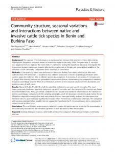
manufacturer would never benefit from deferring leadership. This observation that leadership is beneficial to both the manufacturer and the dealer is consistent with our observation that Wal-mart provides the warranty service for many of the electronics products purchased at its stores while smaller dealers that lack its negotiating leverage often do not. The following Figures 1 and 2 illustrate the profits of the manufacturer and the dealer respectively. In the figures, the parameters are taken as, a = 100, bp = bs = 20, θp = θs = 10 and r = 0.85. Figure 1 gives the manufacturer’s profit where the intersection point between 18
220 210 200
OP T PLP 2−r
T′ 2−r
IN is the equilibrium
190
OP is the 180 equilibrium
OP is the equilibrium
IN
170 160 25
30
35
40
45
50
η
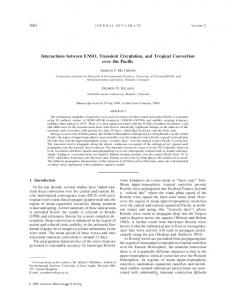
Figure 1: The manufacturer’s profit outcome OP and outcome IN is η1 = 26.1. The manufacturer receives a higher profit for outcome OP when η < 26.1. However, she achieves a larger profit when η > 26.1 for the outcome IN. Figure 2 gives the dealer’s profit. The dealer always gets the highest profit from product line pricing if the manufacturer outsources the service. However, there is an intersection point at η = 47.4 between outcomes IN and IP. If the manufacturer dominates the relationship and decides to insource the service, then the dealer might get a lower profit. Specifically, when 26.1 < η < 47.4, the dealer achieves a lower profit for the equilibrium of IN than that of outcome OP, which is the equilibrium if he is a leader in the relationship.
19
80
78
IP
OP
76
74
IN 45
50
55
60
η
Figure 2: The dealer’s profit
5.
Conclusions
Motivated by observations of differences in how services such as warranty services are delivered to consumers and the extent to which dealers attempt to coordinate pricing decisions across a product line in both the automotive and consumer electronics industries, we have undertaken an investigation of the economic forces that are involved in the relationship between a manufacturer and its dealer. We have focused on two strategic decisions for each of the two firms: the manufacturer’s decision about whether to deliver value adding services directly to the consumer versus delegating this responsibility to the dealer, and the dealer’s decision about whether to decentralize its operations by delegating responsibility for different products to different product managers or centralize its operations. We have shown that by decentralizing, the dealer can credibly signal to the manufacturer that he will adopt a more aggressive pricing policy for the product line, which has the effect of inducing the manufacturer to invest more in service improvement. We have analyzed the subgame perfect equilibrium for the strategic game and found that the equilibrium depends on the market power between the manufacturer and the dealer. A dominant manufacturer would delegate the service to the dealer only when the marginal costs of service provisions were either very low or very high. However, in environments in which the dealer is dominant, we would expect to see the service delivery outsourced to the dealer. 20
There are two main directions in which further research would be fruitful. First, it would be useful to understand how a dealer’s organizational structure and investments in service provisions interact with a manufacturer’s investments in improving the quality of its physical product. Second, it would be useful to understand how a dealer’s decision to centralize or decentralize its operations interact with investment in service improvement when more than one manufacturer is involved.
21
References [1] Banker, R., I. Khosla and K. Sinha. 1998. Quality and competition. Management Science. 44. pp: 1179-1192. [2] Choi, S.C. 1991. Price competition in a channel structure with a common retailer. Marketing Science. 10. pp: 271-297. [3] Cohen, M. A. and S. Whang. 1997. Competing in product and service: a product lifecycle model. Management Science. 43. pp: 535-545. [4] Coughlan, A. T. and B. Wernerfelt. 1989. On credible delegation by oligopolists: a discussion of distribution channel management. it Management Science. 35, pp: 226239. [5] Desiraju, R. and S. Moorthy. 1997. Managing a distribution channel under asymmetric information with performance requirements. Management Science. 43 (12). pp: 16281644. [6] Dixit, Avinish. 1979. A model of duopoly suggesting a theory of entry barriers. Bell Journal of Economics. 10. pp: 20-32. [7] Gilbert, S. M., Y. S. Xia and G. Yu. 2004. The strategic effects of a merger upon supplier interactions. Working paper. [8] Gupta, S. and R. Loulou. 1998. Process innovation, production differentiation, and channel structure: strategic incentives in a duopoly. Marketing Science. 17 (4). pp: 301-316. [9] Harhoff, D. 1996. Strategic spllovers and incentives for research and development. Management Science. 42. pp: 907 - 925. [10] Ingene, C. and M. Parry. 1995. Channel coordination when retailers compete. Marketing Science. 14 (4), pp: 338 - 355. [11] Iyer, G. 1998. Coordination channels under price and non-price competition. Marketing Science. 17 (4), pp: 338 - 355.
22
[12] Jeuland, A. P. and S. M. Shugan. 1983. Managing channel profits. Marketing Science. 2 (3), pp: 239 - 272. [13] Lariviere, M. A. and E. L. Porteus. 2001. Selling to the newsvendor: an analysis of price-only contracts. Manufacturing & Service Operations Management. 3 (4). pp: 293 - 305. [14] Lee, E. and R. Staelin. 1997. Vertical strategic interaction: implications for channel pricing strategy. Marketing Science. 16 (3). pp: 185 - 207. [15] McGuire, T. and R. Staelin. 1983. An industry equilibrium analysis of downstream vertical integration. Marketing Science. 2 (2), pp: 161 - 191. [16] Perry, M. and R. Porter. 1990. Can resale price maintenance franchise fees correct suboptimal levels of retail service. International Journal of Industrial Organization. 8. pp: 115-141. [17] Thomas, M. and S. Rao. 1999. Warranty economic decision models: a summary and some suggested directions for future research. Operations Research. 47. pp: 807 - 820. [18] Trivedi, M. 1998. Distribution channels: an extension of exclusive retailership. Management Science. 44. pp: 896 - 909. [19] Tsay, A. A. and N. Agrawal. 2000. Channel dynamics under price and service competition. Manufacturing & Service Operations Management. 2 (4). pp: 372-391. [20] Winter, R. 1993. Vertical control and price versus nonprice competition. The Quarterly Journal of Economics. 108 (1). pp: 61-76.
23
Appendix b2s (bp +θp ) , such that if (2 − r)η > 2bp θp IN OP then πm < πm , and for T =
Lemma A.1 There exists a synergy threshold level T 0 =
T 0,
IN OP then πm > πm . Alternatively, if (2 − r)η < T 0 ,
T 0,
IN OP πm = πm .
Proof. From Tables 2 and 3, we have: 1 2(bp + θp ) 1 IN OP ) πm − πm = a2 (2 − r)η( − 2 2 2 2 4(2 − r)ηbp − bs θp − bp (bs − 2(2 − r)ηθp ) 2(2 − r)ηbp − b2s Further, the sign of the above equation is determined by the term in the parenthesis which is, f ((2 − r)η) = 2(bp + θp )(2(2 − r)ηbp − b2s ) − (4(2 − r)ηb2p − b2s θp + bp (2(2 − r)ηθp − b2s )) The first derivative of f ((2 − r)η) with respect to (2 − r)η is positive. Therefore, the result follows immediately from the solution to f ((2 − r)η) = 0. IP OP Lemma A.2 πm ≤ πm , that is, if the dealer decides to have product line pricing, the
manufacturer will always outsource the services to the dealer. Thus, outcome IP could never be an equilibrium. Proof. From Tables 2 and 3, it can be observed that, if the dealer uses PLP, the manufacturer will always prefer to outsource the service because:
IP OP πm − πm =−
(2 − r)ηa2 b2s ≤0 2(2(2 − r)ηbp − b2s )(4(2 − r)ηbp − b2s )
24