Strategies for Humanoid Robots to Dynamically Walk over ... - LAAS

1

Strategies for Humanoid Robots to Dynamically Walk over Large Obstacles Olivier Stasse, Bj¨orn Verrelst, Bram Vanderborght and Kazuhito Yokoi1 Abstract— This study proposes a complete solution to make the humanoid robot HRP-2 dynamically step over large obstacles. As compared to previous results using quasi-static stability [1] where the robot crosses over a 15 cm obstacle in 40 s, our solution allows HRP-2 to step over the same obstacle in 4 s. This approach allows the robot to clear obstacles as high as 21% of the robot’s leg length (15 cm) while walking. Simulations show the possibility to step over an obstacle that is 35% of the length(25 cm) with a margin of 3 cm.

0 1 1 0 0 1 0 1 0 1 0 1 0 1 0 1 0 1 0 1 0 1 0 1 0 1 Z ads 0 1 0 1 0 1 0 1 0 1 0 1 0 1 0 1 0 1 0 1 0 1 0 1 0 1 0 1 0 1 0 1 0 1 0 1 0 1

0000000X ads 1111111 1111 0000 11 00 1 X hds 0

L1

L7

L6 O3 1 0 00 11 0 1 00 11 0 1 00 11 0 1 000 111 1 0 0 0 1 000 111 1 Sh O2111 000 000 111 000 L5 111 000 111 Ow Oh 000 111 1111 0000 000 111 000 111 O1 1 O4 1 0 11 00 Sw 000 111 0 000 111 000 111 0 1 000 111

L2

L3

L4

1111 0000 0000 1111 0000 1111 0000 1111 0000 1111 0000 1111

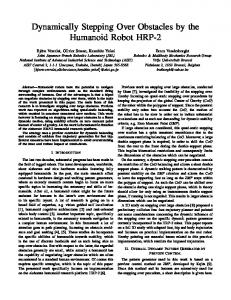
Fig. 1. The key configuration in the doublesupport phase with parameters Xhds , Xads , and Zhds .

Index Terms— Humanoid Robots, Obstacle Negotiation, Trajectory Planning

I. I NTRODUCTION In path planning for humanoid robots, obstacle avoidance and goal seeking [2], [3], [4], [5], [6] incorporate the specific abilities of humanoid robots to step over obstacles. Generally, the obstacles considered are small, although a humanoid robot actually has the capability of negotiating larger obstacles often encountered in a standard human environment. There are wellknown examples of robots that can smoothly step over small obstacles, such as Johnnie [7] (5 cm obstacles) and ASIMO [8] (flat obstacles). Recent studies have reported on the stepping over capabilities of the BHR-2 humanoid robot [9]. Related studies reported on achieving jumping motions using legged robots. Such robots are highly dynamic and can move on irregular terrains. The best known examples were developed by Raibert [10] in the 1980s, who realized large jumping motions using robots with telescopic legs. Thus far, these studies have not involved the negotiation of large obstacles. Previous studies on stepping over large obstacles, conducted by Guan et al., investigated the feasibility of stepping over [1] and performed experiments using the HRP-2 robot [11]. This study focuses on quasi-static stepping over procedures by keeping the projection of the total Center of Mass (CoM) of the robot within the support polygon. Since the postural stability only considers the CoM, the motion of the robot has to be slow in order to avoid inducing substantial accelerations and as such, it does not involve dynamic stability criteria, e.g., for instance the Zero Moment Point (ZMP) [12]. Here, we propose improvements in the capabilities of HRP2 to walk over obstacles by implementing dynamic motions instead of using a quasi-static approach. This has an advantage in that the robot does not need to come to a complete stop before negotiating an obstacle, and higher obstacles can be negotiated faster. The method presented here relies on the work of Kajita et al. [13] and it implements some key techniques that allow stepping over large obstacles. Our main contributions are as follows: 1 B. Verrelst was at the CNRS-AIST Joint Robotics Laboratory (JRL), UMI 3218/CRT, AIST Central 2, 1-1-1 Umezono, Tsukuba, Ibaraki, Japan 305-8568 during this study. O. Stasse and K. Yokoi are also at the JRL. B. Verrelst and B. Vanderborght are at the Robotics & Multibody Mechanics Research Group, Vrije Universiteit Brussel Pleinlaan 2, 1050 Brussel, Belgium. email: {bjorn.verrelst, bram.vanderborght}@vub.ac.be, {olivier.stasse, kazuhito.yokoi}@aist.go.jp

1) determine the CoM height trajectory necessary to step over obstacles along with a dynamic pattern generator; 2) experimentally show that it is possible to dynamically step over obstacles as large as 15 cm × 5 cm, and deal with impacts at the planning level; 3) show via simulation that the robot can clear an obstacle having dimensions of 25 cm × 5cm. Walking dynamically allows also the robot to have a very short double-support phase, as shown by the key configuration depicted in Fig.1. This configuration has three parameters Xads the step length , Xhds the distance between the rear foot and the waist, and Zhds the waist height from the ground. It is constrained by the robot shape represented by the lines connecting the points Li , i = 1, ...7, and the obstacle Oj , j = 1, ..., 4. Section II presents some important remarks based on a simple formulation of the problem. Section III describes the trajectory generator. The simulation results described in Section IV show that, HRP-2 can even step over 25-cm-high obstacles. The experimental successfulness of the proposed trajectory generator is described in Section V. It shows that HRP-2 is capable of dynamically stepping over a 15-cm-high obstacle with a safety margin of 3 cm. II. P ROBLEM S TATEMENT Following Guan et al. [1], stepping over an obstacle is defined by three phases: Phase 1 is a single-support phase and involves putting one foot in the rear of the obstacle. Phase 2 is a double-support phase where both feet are on the ground and on each side of the obstacle. Phase 3 is a singlesupport phase where the rear foot is brought over the obstacle. As compared to normal walking, additional constraints have to be imposed on the motion: (1) collision free constraint, (2) kinematic limits, (3) stability and, (4) impact reduction constraint. Constraints 1 and 2 are quite obvious. Guan et al. [1] considered the quasi-static stability criteria for the balance constraint 3. The motion generated was quite slow and thus did not consider constraint 4. A. Stepping over with quasi-static constraints In order to illustrate the relationship between the kinematics and stability constraints, let us consider a 2D bipedal model

TRANSACTION ON ROBOTICS, SHORT PAPER, CORRESPONDING AUTHOR: OLIVIER STASSE

with c = [cx , cy , cz ]⊤ , the Center of Mass of the robot; and T P i , the time when phase i finishes. The joint trajectories during phase i are denoted by qP i (t). While (1) is the constraint on the joint limits, (2) states the continuity of the poses between the phases, (3)-(4) state that this a double support phase, (5) represent the constraints to avoid collision with an obstacle, (6) is the stability constraint at end of phase 1, (7) is the stability constraint during phase 2 and (8) is the stability constraint at the beginning of phase 3. Axi xi+1 oj oj+1 is the crossproduct defined by: −−→(t) × − −−→(t) (t) = − x−x o−o (9) A xi xi+1 oj oj+1

i i+1

j j+1

−−−−→ −−→ x− where Axi xi+1 oj oj+1 < 0 if and only if − i xi+1 and oj oj+1 intersect [14]. From (4), two degrees of freedom are fixed by setting x1z (t) = 0 and x5z (t) = 0, and by fixing x1 at the origin, a third one is fixed; thus, 3 DOFs are left. The remaining 3 DOFs can be used on imposing conditions on the parameters Xads , Xhds , and Zhds . In Fig.2 we have plotted the domain for which, given a pair (Xads , Zhds ), it is ⊤ possible to find a corresponding [Xhds q(t)⊤ ]⊤ that satisfies the constraints. From those graphs, we can formulate the following remarks: Remark 1: The domain of a solution for phase 2 of stepping over with quasi-static criteria is mostly limited at the beginning (upper graph in Fig.2) and the end (lower graph in Fig.2). Remark 2: Let us consider the constraint given by (7), and the feasibility domain plotted in the middle graph of Fig.2. It appears that when Zhds ∈ [0.47, 0.7], lowering Zhds increases the domain of Xads . Those two remarks are in agreement with the work of Guan et al. [1], who found a critical configuration at the beginning of phase 2 (Fig.9, p.964), and lowered the waist height if the inverse kinematics failed (Fig.14, p.968). Remark 3: Finally, it appears that once a suitable Xads is found, phase 1 mostly involves finding a trajectory for the first foot (x5 ) while having the robot having its CoM under the

x3

l2

q

3

Feasibility domain at beginning of Phase 2 with quasi static stability

l3

q2

x4

x2

o2

x1

Y

0.7 0.6

l4

q1

q4 x5

o1

X

0.8

o3

l1 Z

Z hds

Zhds

Xhds

0.4

0.2

Fw

Fw

0.5

0.3

o4

0.1 0.0 0.0

Xads Feasibility domain during Phase 2 with quasi static stability

0.8

0.8

0.7

0.7

0.6

0.6

0.5

0.5

0.4

0.4

0.6

0.8 Xads

1.0

1.2 1.3

0.4

0.3

0.3

0.2

0.2

0.1

0.2

Feasibility domain at the end of Phase 2 with quasi static stability

Zhds

with 4 links l = {l1 , l2 , l3 , l4 }, its 4 related joints q = {q1 , q2 , q3 , q4 }, and the corresponding position in the Cartesian space x = {x1 , x2 , x3 , x4 , x5 } (cf. Fig.2). Let us now focus on phase 2 of the stepping over, i.e. when the robot is in the double-support phase, this will be helpfull to consider phase 1 and phase 3. For the quasi-static case, the goal of stepping over is to find a trajectory [x1 (t)⊤ q(t)⊤ ]⊤ such that the following constraints are met during phase 2, i.e., ∀ t ∈ [T P 1 ; T P 2 ] unless specified otherwise:  qmin ≤ qP 2 (t) ≤ qmax (1)    P1 P1 P2 P1 P2 P2 P3 P2   q (T ) = q (T ), q (T ) = q (T ) (2)    2 P1 P1 2 P1 P1   xP ), xP ) (3)  1 (t) = x1 (T 5 (t) = x5 (T   P1 P2 P2 P2   (t) = 0, ∀ t ∈ [T ; T ] (4) (t) = x x  5z 1   z Axi xi+1 oj oj+1 < 0, ∀i ∈ {1, 2, 3, 4}∀j ∈ {1, 2, 3} (5)  FW FW   ≤ cxP 2 (T P 1 ) ≤ (6) −    2 2    FW FW   − ≤ cxP 2 (t) ≤ Xads + , ∀ t ∈]T P 1 ; T P 2 [ (7)   2 2     FW  − FW + X P2 P2 ) ≤ Xads + (8) ads ≤ cx (T 2 2

Zhds

2

0.1

0.0

0.0 0.0

0.2

0.4

0.6

0.8 Xads

1.0

1.2 1.3

0.0

0.2

0.4

0.6

0.8 Xads

1.0

1.2 1.3

Fig. 2. (top left) Simple model of a 2D bipedal robot in the double-support phase. The other graphs depicts its feasibility domain as follows: red depicts a feasible combination, while blue states a combination for which at least one constraint is always violated. The right-upper graph correspond to the case where the constraint given by (6) is violated. The right bottom graph correspond to the case where the constraint given by (8) is violated. The obstacle considered here is 5 × 15 cm.

constraint of (6). Conversely, phase 3 mostly involves finding a trajectory for the second foot (x1 ) while having the robot having its CoM under the constraint of (8). B. Stepping over with dynamical stable constraints 1) Single mass model: The stability criteria considered in this work is the ZMP, and it is written as p = [px , py , pz ]⊤ . Hence, from the previous set of constraints (1)-(8), the quasistatic constraints (6)-(8) should be changed to the following equations:  F FW W 2 P1  ≤ pP )≤ (10) −  x (T   2 2    FW  FW 2 − ≤ pP , ∀ t ∈]T P 1 ; T P 2 [(11) x (t) ≤ Xads + 2 2   F FW  2 P2  − W + Xads ≤ pP ) ≤ Xads + (12)  x (T  2   P 22 P 1 p (T ) = pP 1 (T P 1 ), pP 3 (T P 2 ) = pP 2 (T P 2 )(13)

Because this is a dynamic constraint, we now have to ensure the continuity with (13). Then the problem is to find a trajectory [x1 (t)⊤ q(t)⊤ ]⊤ . Let us recall some standard results on bipedal walking. The first assumption is to assume that the robot can be reduced to a point mass to which one contact force and gravity is applied. This assumption is admissible for a robot such as HRP-2 because 72% of its mass is in the upper body2 . From this assumption, the robot’s simplified model can be written as: mgcx + pz m¨ cx − m(cz c¨x − cx c¨z ) (14) px = mg + m¨ cz

2 However, a robot having heavy legs cannot neglect the inertial effect induced by the swinging legs. This usually necessitates more complex models than the single mass model[15].

3 0.28

⊤ L with pN x (k + 1) . . . px (k + NL )] , cx (k) = x (k + 1) = [p... ... ... ⊤ c NL [cx (k) c˙x (k) c¨x (k)] , x (k) = [ c x (k) . . . c x (k + NL )]⊤ , and Px and Pu are matrices built upon the stack of NL (15). ... L The control, written as c N x , minimizes:

1 ... 2 1 Q(px (k + 1) − pref1 (k + 1))2 + R c NL x (k) (17) min ... NL 2 2 c (k) x

This can be solved analytically by: R ...NL 1 c x (k) = −(PTu Pu + I)−1 PTu (Px cx (k)−pref (k)) (18) x Q where I is an identity matrix; Q, the gain for the preview win1 , the ZMP reference dow; R, the gain for the command; pref x trajectory defined from Xads and Xhds . The discrepancies between the single mass model (15) and the multibody robot’s model are compensated by a second stage of (16). The ZMP reference is given by B 1 2 (k) − pM (k) (k) = pref pref x x x B (k) pM x

(19)

is the ZMP along the x-axis computed using where the robot multibody model. The result is a difference added to cx (k). In addition to the multibody model, this second stage compensates for the variation introduced by the planning of cz , and some motions introduced in section III-D. 3) Key configuration: Considering the CoM trajectory generated by the preview control during the double-support phase, which is very short as compared to the quasi-static phase (40 ms instead of 15 s), the range of motion is very small 5 mm, as will be seen in Section V. Contribution 2: Thus, the disadvantage suggested by remark 1 with regard to the quasi-static stepping over does not

Adapted Classical

0.26 0.24 0.22 Height (m)

where m is the mass of the robot. Then a standard is to impose other constraint to solve (14) in real-time. Here, we describe the linearization of this equation. Imposing z¨ = 0 leads to the linear inverted pendulum also called as the cart model: c¨x (pz − cz ) px = cx + (15) g Remark 4: For a robot with a mass distribution equivalent to that of HRP-2, the relationship between the CoM height and the waist height can be approximated by x3z = cz + cst. Therefore, considering the second graph of Fig.2, the feasibility domain for Xads is the segment defined by the line Zhds = x3z = cz + cst. Of course, this considerably reduces the feasibility domain. Practically, however, recent works by Kajita et al. [16] and Morisawa et al. [17] have shown that it is possible to modify cz provided that c¨z is sufficiently small to satisfy (15). Contribution 1: Considering remarks 2 and 4, we propose to extend the feasibility domain to step over dynamically for a robot reduced to a linearized inverted pendulum by planning the CoM height under the assumption that c¨z ≪ g. 2) CoM trajectory generation and multibody model: Let us recall the preview control method [13] using Wieber notations [18]. First, the system described by (15) over NL iterations is written as: ...NL L (16) pN x (k + 1) = Px cx (k) + Pu c x (k)

0.2 0.18 0.14 0.15 0.12 0.1 0

Fig. 3.

0.2

0.4

0.6

0.8

1 1.2 Time (s)

1.4

1.6

1.8

2

Foot trajectories adaptation to minimize impact

apply in this case. Moreover, as the variation is quite small, the double-support phase trajectory can be reduced to one position that we call the key configuration. Finally, based on remark 3, we assume, for now, that with a robot similar to our simplified model once the key configuration is found, the generation of phase 1 and 2 is a direct application of the preview control with the foot trajectory generation described in paragraph III-B. Paragraph III-E proposes a solution when this assumption does not hold anymore. In order to have a clear view of the other constraints to maintain the assumption of (15), let us consider the 3D version of (14): px =

mgcy + pz P˙ y − L˙ x mgcx + pz P˙ x − L˙ y , py = mg + P˙ z mg + P˙ z

(20)

where Px is the linear momentum along the x-axis and Lx the angular momentum around the x-axis. The same notation is used for the momentum related to the other axes. In order to maintain (15), i.e., decoupling of the axes between each other, we should impose L˙ = [mcz c¨y mcz c¨x 0]⊤

(21)

with the trajectory of the CoM given by the preview control [13]. Kajita et al. [19] proposed a controller based on a L reference. However, to avoid a collision with the obstacle we also have to ensure that the key configuration Xads , Xhds and Zhds found is not changed. Therefore, when using such a controller, we would have to impose the position of the waist and the legs’ articular values. Consequently, considering the mass distribution of the robot, we are assuming that by maintaining the upper part of the robot under the constraint given by (21), the use of the dynamic filter in the preview control method and our foot trajectory strategies are sufficient to satisfy (15). This is confirmed by the experiments described in Section V. C. Impact reduction constraint Avoiding high-impact shocks at landing is a recurrent problem in bipeds. The feet of HRP-2 [20] or ASIMO have rubbers between the surface in contact with the floor and the force sensor, as depicted in Fig.3. The passive joint added to the system is then compensated by using the commercial stabilizer

4

TRANSACTION ON ROBOTICS, SHORT PAPER, CORRESPONDING AUTHOR: OLIVIER STASSE

Feasibility Unit (FU)

ow oh sw sh

Xads Xhds

L1 Feet Trajectory Generator (FTG)

ZMPdes

Z hds CoM and Waist Traj. Generator (CWTG 1) L R W

Feet Trajectory Adaptator (FTA)

R1

W2 CoM 2

W1 CoM1 CoM and Waist Traj. Generator (CWTG 2)

Inverse Kinematics (IK) Upper Body Motion Generator (UBMG)

Legs 1 W1 UB 1

ZMPdes

L1

Fig. 4.

The overall algorithm for stepping over obstacles

of HRP-2, on which no information is currently available. However, the stepping over mechanism proposed in this paper generates a large step-length (40 cm in the case of a 15-cmhigh obstacle, whereas the standard length is 20 cm). Using a fourth order polynomial for the height-foot trajectory (x5 in the simplified model) has two disadvantages: the swinging foot has a zero velocity late in phase 1, and because of the lack of control points, the velocity is quite important. The stabilizer is not able to compensate properly for the flexibility at the end of phase 1. Thus, the dashed trajectory depicted in Fig.3. is slightly rotated, and the foot hits the floor with a non-zero speed. The impact of the foot measured in this case is twice the weight of the robot. Because we are bound to keep the commercial stabilizer, we propose to shape the foot trajectory such it has a low-velocity phase before landing. Having a high speed for the foot makes its inertial effect not negligible, and the assumption given by (21) does not hold. Reducing the speed avoids the compression of the flexible material. This is dealt with by the Feet Trajectory Generator. III. S TEPPING OVER TRAJECTORY GENERATOR The obstacle is regarded to be rectangular with width ow = ||o2 − o3 || and height oh = ||o2 − o1 || (as depicted in Fig.1). For the stepping over trajectory planning, a safety margin (sw , sh ) around the obstacle is included. This margin cope with the uncertainty related to tracking and measurement errors. The computation giving the trajectories of the legs (L(t), R(t)), waist W (t), CoM CoM (t), and the upper body U B(t) is described by Algorithm 1 and depicted in Fig.4. Algorithm 1 (L(t), R(t), W (t), CoM (t), U B(t)) ← SteppingOverObstacle(ow , oh , sw , sh ) 1. (Xads , Xhds , Zhds ) ← F U (ow , oh , sw , sh ) 2. (L1 (t), R1 (t), ZM Pdes (t)) ← F T G(ow , oh , sw , sh , Xads , Xhds ) 3. (CoM1 (t), W1 (t)) ← CW T G1(ZM Pdes , Zhds ) 4. Legs(t) ← IK(L1 (t), R1 (t), W1 (t)) 5. U B(t) ← U BM G(CoM1 (t), W1 (t)) 6. (CoM (t), W2 (t)) ← CW T G2(ZM Pdes (t), Legs(t), U B(t), L1 (t), R1 (t)) 7. (L(t), R(t), W (t)) ← F T A(L1 (t), R1 (t), W2 (t)) The Feasibility Unit (FU) calculates the required step-length (Xads ), hip-forward position (Xhds ), and hip-height (Zhds )

based on the kinematic and collision free constraints. Using the foothold positions, the feet trajectories (L1 (t), R1 (t)) and the desired ZMP trajectory (ZM Pdes (t)) are calculated by the Feet Trajectory Generator (FTG); this requires the collisionfree and impact-reduction constraints. Subsequently, the CoM and the Waist Trajectory Generator (CWTG) calculates the horizontal and vertical CoM motions (CoM1 (t)) and the waist trajectory (W1 (t)). The preview method calculates the horizontal CoM motion considering the balance constraints. The vertical CoM motion is calculated from the required hip height (Zhds ) during the double-support phase. Using the feet trajectories and the waist trajectory, we can then compute the leg joint trajectories (Legs(t)) by using Inverse Kinematics (IK). To avoid knee over-stretch, the Upper Body Motion Generator (UBMG) let the arm swing to create a variation of CoM; we thus define the upper body joint trajectories (U B(t)) accordingly. These trajectories are then checked against collisions. The CoM height trajectory is modified accordingly, and finally, using the second stage of preview control proposed by Kajita et al. [13], a new CoM horizontal trajectory is generated. Those operations are realized by the second CoM and Waist Trajectory Generator (CWTG2). Finally, the Feet Trajectory Adaptor (FTA) adapts the feet trajectory to cope with intermediate collisions and consequently considers the collision constraints. The trajectories of the feet L(t), R(t), CoM CoM (t), waist W (t) and arm trajectories U B(t) describe the complete motion of the robot. The inverse kinematic unit calculates the different joint trajectories that are adapted by the stabilizer before sending them to the local motor controllers. Each unit is now discussed in more detail.

A. Feasibility Unit (FU) The feasibility unit is a kinematical study that calculates if an obstacle can be negotiated or not. If possible, it provides a collision-free configuration by determining the step-length (Xads ) and the waist-height (Zhds ). This configuration is called the key configuration. The selection of these parameters begins with a minimal step length and normal-walking waist height. In the case of a collision, the step length is increased and the waist height is decreased until a collision-free configuration is found. The geometrical model used is a simplification of HRP-2’s full model for fast collision checking [21]. It is based on line segments such as the ones depicted by points Li i = 1, ..., 7 in Fig.1. Theoretically, for each (Xads ), the associated ZMP and CoM trajectories should be computed in order to obtain the proper Xhds . However, this would be very time consuming. Therefore, we use a parameter δDS given as: Xhds = δDS Xads

(22)

The value of parameter δDS originates from simulations for normal walking with an estimation for different step-lengths using (16). Simulations show that the value of δDS does not vary significantly when stepping over is considered. We believe that finding this parameter, or a look-up-table, for other robots is feasible (here, δDS = 0.5). More information about this unit can be found in [21].

5

B. Feet Trajectory Generator (FTG) For the three translations and pitch rotation of the foot, clamped cubic splines (CCS) are chosen over the more traditional polynomials because the later tend to oscillate when different control points are chosen. The control points are introduced according to the step-length (Xads ) and the obstacle dimension. In order to lower the impact at touch down, intermediate points are added to obtain a decreasing linear distribution of the speed over the trajectory, as depicted in Fig.3. The impact force was reduced from 1200 N to 625 N, which is 1.1 times the robot’s weight. A detailed description of the trajectory generator which allows avoiding the obstacle and controlling the speed can be found in [22].

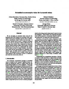
Fig. 5. Stick diagram of HRP showing intersection of the rear leg with the boundary of the obstacle

C. CoM and Waist Trajectory Generator (CWTG1)

D. Upper body motion generator (UBMG) and Second CoM and Waist Trajectory Generator (CWTG2) Using the 3 units described above, the stepping over trajectory generator can negotiate obstacles up to a height of 20 cm. For higher obstacles, near overstretching must be avoided, specifically during experiments, as we observed that the extra stabilizing control loop [23], currently implemented in the HRP-2 robot, generates high accelerations in this situation. These high accelerations trigger the robot’s low-level security system.

ZMP and waist positions (m)

Waist Position Before Waist Adaption

1,6

Waist Position Final

1,4

X ZMPdesired

1,2 1 0,8

Double support over obstacle

0,6 0,4 0,2 0 0

1

2

3

4

5

6

7

8

9

10

Time (s)

2

Foot positions (m)

1) Vertical Waist trajectory: The waist-height selection requires planning of the vertical waist motion, which has to be changed (lowered) from the normal walking height to reach (Zhds ) during the double support over the obstacle, which was determined by the feasibility study. During the step over of the first leg, the waist is lowered such that it reaches Zhds . Subsequently, it is raised during the second step. Both motions are achieved by regular third order polynomials that include boundary conditions at the position and velocity levels. Note that as long as the condition c¨z ≪ g is satisfied, we can independently plan the height from the other two axes. 2) Horizontal CoM trajectory: The horizontal CoM motion is calculated from the desired ZMP trajectory and the feet trajectories using the first stage of the ZMP preview control method [13]. This implies that only the point mass model specified in (15) is considered at this stage. L1 (t) and R1 (t) are used to compute the ZMP desired trajectory. 3) Rotational waist motion: In order to clear more space during the double support over the obstacle and consequently allow for larger obstacles to be stepped over, the waist of the robot is rotated. The HRP-2 robot includes 2 extra DOFs (yaw and pitch) between the waist and upper body; thus the yaw angle is rotated such that the waist is not parallel to the obstacle anymore while the upper body and head (with vision system) are still oriented towards the walking direction. We experimentally determined that the condition L¨z ≡ 0 is verified because of the HRP-2 mass distribution when its the upper body does not move. This motion is achieved with an analogous polynomial structure as in the case of the vertical waist motion.

2 1,8

Left Foot Positions X Before Adaptation

Left Foot Positions X Final

1,8

Left Foot Positions Z Before Adaption

Left Foot Positions Z Final

1,6

right foot positions

X ZMPdesired

1,4 1,2 1 0,8

Double support over obstacle

0,6 0,4 0,2 0 0

1

2

3

4

5

6

7

8

9

10

Time (s)

Fig. 7. Stepping over a 25-cm-high and 5-cm-wide obstacle of (plus 3 cm safety boundary - 2 × 3 cm safety boundary, respectively): ZMP and waist position in walking direction (X) and horizontal and vertical foot positions

The knee-over-stretch of the swinging leg during the first step occurs due to the fact that the waist has not moved sufficiently far to the front with respect to the foot motion. If the CoM of the robot is shifted to the rear by a specifically chosen upper body motion, the dynamic filter (19) compensates for the shift on the total CoM by moving the waist forward in order to maintain the desired ZMP. If the perturbation is ... 2 (k) < 0, it in turn allows c x (k) > 0 in such that pref x (18) for generating a forward motion of the waist. This is realized by creating a backward motion of the arm so that B 1 (k) < pM (k). It is not possible to use the chest as the pref x x robot is limited with this joint in the backward direction.

6

TRANSACTION ON ROBOTICS, SHORT PAPER, CORRESPONDING AUTHOR: OLIVIER STASSE

(1) First Step P1 Fig. 6.

(2) No Overstretch

(3) Double Support

(4) No Intersection

(5) No Intersection

Snapshots of the step over procedure for an obstacle of 25 cm plus 3 cm safety boundary zone after waist and foot trajectory adaptation

E. Feet trajectory adaptor (FTA) There is no guarantee that finding the key configuration in the feasibility unit will result in collision-free stepping over since it only provides a collision-free double-support phase. This especially occurs when large obstacles are negotiated, due to the complex movement and the shape of the leg itself. Therefore, the last tool required is a trajectory adapter that makes small corrections to the planned base trajectories. This mainly acts during the third phase of the motion (i.e., second leg stepping over). Indeed, the knee intersects the safety boundary on top of the obstacle, as depicted in Fig.5. In order to detect collisions, the line segments on the leg (L1 , ..., L7 ) and the obstacles (O1 , ..., O4 ) depicted in Fig.1 are used, as described in [1]. Three methods are presented to modify the foot trajectory appropriately: (1) modifying the foot trajectory, (2) modifying the height of the waist, and (3) using a penetration distance based controller. 1) Foot trajectory modification: The swinging foot trajectory is modified by shifting the horizontal position to the rear until no collision occurs. 2) Waist height modification: In addition to the foot trajectory alteration, the waist height trajectory is increased such that the knee does not intersect the safety boundary on top of the obstacle. After applying the waist-height variations, collisions may still occur, and thus the foot trajectory is adapted incrementally. 3) Controller on penetration distance: During phase 3 if a collision occurs between the lift-off leg and the obstacle, a horizontal penetration vector dS is calculated. Subsequently, an appropriate ankle displacement vector dP is computed in order to avoid the intersection with the boundary around the obstacle. It is assumed that the calculated penetration dS is small whenever a collision is detected. Therefore, Jacobian calculations can be used to link the displacements dS and dP. The joints angles of the HRP-2 robot legs are represented by q, and dq denotes the displacement dP. Analogous dS and dP are expressed with respect to a coordinate frame attached to the waist: dS = Js dq

(23)

dP = Jp dq

(24)

The Jacobian matrix Js is calculated starting from the intersection point with the safety boundary around the obstacle and Jp always from the ankle point. Thus, eliminating the vector changes dq in (23) and (24) gives: dP = Jp Js+ dS

(25)

where Js+ a (Moore-Penrose) pseudo-inverse of Js since the latter has dimensions of 3 × 4. An animation of the upper body motion and the proposed adaptation of the foot is shown in Fig.6 and can also be seen in the accompanying video. The backwards arm motion to avoid knee-over-stretch, and the extra yaw waist rotation to clear more space between the legs during double support over the obstacle, can be clearly seen in the animation. IV. S IMULATION R ESULTS In this section, we present simulation results in which HRP2 is able to step over higher obstacles than those during experiments. The upper part of Fig.7 shows the waist trajectory adaptation considering an obstacle of 25-cm-high and 5-cmwide (with 3 cm safety boundary and 2×3 cm safety boundary, respectively). It can be seen that the waist is more towards the rear than before the adaptation, which induces the overstretch. The bottom part depicts the modification of the foot trajectory adaptor on the left foot trajectory during phase 3. The foot lift is clearly higher after adaptation to cope with the high obstacle. Accordingly, the step-length initially calculated by the feasibility tool is larger after the foot adaptation. The ZMP trajectory shows that the overall stability is guaranteed by the dynamic filter. During these simulations speed and torque motor limits are not present. V. E XPERIMENTAL R ESULTS The results of stepping over an 15-cm-high and 5-cm-wide (with a 3 cm safety boundary and 2x3 cm safety boundary, respectively) are depicted in Fig.8, Fig.9 and Fig.10, The figures show the desired ZMP and waist position for both the walking direction (X) and the perpendicular horizontal direction (Y) (showing 7 steps). A normal step takes 0.78 s for single support and 0.02 s for double support, while the stepping over step and both previous and subsequent steps take 1.5 s and 0.04 s respectively. The stability of the system

7

2 ZMP MultiBody X First Preview

1,8 ZMP and waist positions (m)

ZMPMultiBody X Second Preview 1,6

Waist Position X

1,4 1,2 1 0,8

Double support over obstacle

0,6 0,4 0,2 0 0

1

2

3

4

5

6

7

8

9

10

Time (s) 2 Left Foot Positions X Right Foot Positions X X ZMP desired

1,8

Foot positions (m)

1,6

Left Foot Positions Z Right Foot Positions Z

1,4 1,2 1 0,8

Double support over obstacle

0,6 0,4 0,2 0 0

1

2

3

4

5

6

7

8

9

10

Time (s)

Fig. 8. ZMP and waist position in the walking direction(X), including horizontal and vertical foot positions, for stepping over a 15-cm-high and 5-cm-wide (plus 3 cm safety boundary and plus 2 × 3 cm safety boundary, respectively)

0,12

ZMP desired Y

Waist position Y

0,08 ZMP and waist position (m)

is given by the position of the ZMP, which is calculated using the complete multi-body model of the robot. The bottom graphs in Fig.9 show both the ZMP calculations after the first and second preview controllers. The first preview is clearly jerky and different from the desired ZMP, specifically for the stepping over. However the dynamic filter (second preview control) compensates completely for the use of the simplified model, the disturbances of the large swing leg motions and the waist height variation during the stepping over. It is particularly important in this direction because this is where the largest perturbations occur, while the support area is the shortest. The accompanying video shows several motions over different obstacles. The obstacle limit for real experiments thus far is 15 cm mainly due to the following reasons. An important influencing factor is the presence of the extra stabilizing control loop [23]. The preview pattern generator considers the complete multi-body model of the robot but does not include model parameter errors, compliance of the feet, extra external perturbations, etc. Therefore, the stabilizer acts on the posture of the robot try to match the real measured ZMP with the desired one. This feedback loop controls the waist motions and consequently the leg stance configuration; further it adapts the swing leg according to the changing waist position. Consequently, even if near over-stretch situations are carefully avoided by the step over planner, the stabilizer tends to induce high accelerations and saturates the motor torque. This creates a tracking error that triggers HRP-2’s security system into automatically cutting the power supply. For stepping over a 20-cm-high obstacle, this limitation was reached, e.g., in the knee of the second swing leg stepping over the obstacle. This is also the reason why a compensating arm motion to the rear, as discussed in section III-D, is provided in the experiments. The computation time of the planning phase is 400 ms for this obstacle, i.e., steps 1 and 2 of algorithm 1. Steps 3 to 7 are computed online, and each iteration takes 0.5 ms in HRP-2. However, it is important to note that step 7 requires no time as there is no collision for this obstacle’s size and therefore is not activated.

0,04

0 0

1

2

3

4

5

6

7

8

9

10

-0,04

-0,08

-0,12

Double support over obstacle

Time (s)

VI. C ONCLUSIONS 0,12

ZMP MultiBody Y First Preview

ZMP MultiBody Y Second Preview

0,08

ZMP position (m)

This paper reports on dynamically stepping over large obstacles using the humanoid robot HRP-2. The key to clearing large obstacles is in shortening the double-support phase and lowering the CoM height using a dynamical walking pattern generator. We described a method to modify the feet trajectory and upper body motion that considers obstacle avoidance, joint limits, dynamical stability, and impact. The different units of the stepping over trajectory generator were discussed in detail. Due to the limitations of the commercially available ZMP controller, 15 cm (with the addition of the 3 cm boundary values) is currently the maximum height for HRP-2 in an experiment. However we have shown through simulation that HRP-2 can step over a 25-cm-high and 5-cm-wide (with the addition of the 3 cm boundary values) obstacle using the proposed strategy.

0,04

0 0

1

2

3

4

5

6

7

8

9

10

-0,04

-0,08

-0,12 Time (s)

Fig. 9. ZMP and waist position of the perpendicular horizontal (Y) direction for stepping over an obstacle of 15-cm-high and 5-cm-wide (plus 3 cm safety boundary and plus 2 × 3 cm safety boundary, respectively)

8

TRANSACTION ON ROBOTICS, SHORT PAPER, CORRESPONDING AUTHOR: OLIVIER STASSE

Fig. 10. Photograph sequence of HRP-2 stepping over an obstacle of 15-cm-high and 5-cm-wide (18-cm height and 11-cm width including safety boundaries). The images are taken every 0.64 s

Currently, the stepping over procedure is being integrated with several other walking modes and behaviors in the real robot. It has been routinely demonstrated to visitors, and has been tested on a different HRP-2. In the future a vision system will be integrated to detect obstacle dimensions and position. ACKNOWLEDGMENT This research was supported by a post-doctoral fellowship of the Japan Society for Promotion of Science (JSPS). Bram Vanderborght received a grant from the Fund for Scientific Research-Flanders (Belgium, FWO). The authors would like to thanks P.B. Wieber, F. Lamiraux and N. Mansard for remarks and discussions. R EFERENCES [1] Y. Guan, K. Yokoi, and K. Tanie, “Feasibility: Can humanoid robots overcome given obstacles ?” in IEEE ICRA, April 2005, pp. 1066–1071. [2] R. Cupec and G. Schmidt, “An approach to environment modelling for biped walking robots,” in IEEE IROS., 2005, pp. 3089–3094. [3] O. Lorch, A. Albert, J. Denk, M. Gerecke, R. Cupec, J. Seara, W. Gerth, and G. Schmidt, “Experiments in vision-guided biped walking,” in IEEE IROS, 2002, pp. 2484–2490. [4] J. Chestnutt, J. Kuffner, K. Nishiwaki, and S. Kagami, “Planning biped navigation strategies in complex environments,” in IEEE Intl.Conf. on Humanoid Robots, 2003, pp. 13–18. [5] J. Seara, K. Strobl, and G. Schmidt, “Information managment for gaze control in vision guided biped walking,” in IEEE/RSJ IROS., 2002, pp. 31–36. [6] M. Yagi and V. Lumelsky, “Biped robot locomotion in scenes with unknown obstacles,” in IEEE ICRA, 1999, pp. 375–380. [7] J. F. Seara, O. Lorch, and G. Schmidt, “Gaze control for goal-oriented humanoid walking,” in IEEE-RAS Intl.Conf. on Humanoid Robots, 2001. [8] P. Michel, J. Chestnutt, J. Kuffner, and T. Kanade, “Vision-guided humanoid footstep planning for dynamic environments,” in IEEE-RAS Intl.Conf. on Humanoid Robots, December 2005, pp. 13–18. [9] A. R. Jarfi, Q. Huang, L. Zhang, J. Yang, Z. Wang, and S. Lv, “Realization and trajectory planning for obstacle stepping over by humanoid robot bhr-2,” in IEEE Intl.Conf. on Robotics and Biomimetics, 2006, pp. 1348–1354.

[10] M. Raibert, Legged Robots That Balance. MIT Press, Cambridge, Massachussetts, 1986. [11] Y. Guan, N. Ee Sian, K. Yokoi, and K. Tanie, “Stepping over obstacles with humanoid robots,” IEEE Transactions on Robotics, vol. 22, no. 5, pp. 958–973, 2006. [12] M. Vukobratovic and B. Borovac, “Zero-moment point - thirty five years of its life,” International Journal of Humanoid Robotics, vol. 1, pp. 157– 173, 2004. [13] S. Kajita, K. Kanehiro, K. Kaneko, K. Fujiwara, K. Harada, K. Yokoi, and H. Hirukawa, “Biped walking pattern generation by using preview control of zero-moment point,” in IEEE ICRA, 2003, pp. 1620–1626. [14] T. H. Cormen, C. E. Leiserson, and R. L. Rivest, Introduction to Algorithms. Mc Graw Hill, 1996. [15] T. Buschmann, S. Lohmeier, M. Bachmayer, H. Ulbrich, and F. Pfeiffer, “A collocation method for real-time walking pattern generation,” in IEEE/RAS International Conference on Humanoid Robotics, 2007, p. 44. [16] S. Kajita, Humanoid Robot. Omsha, 2005, (In Japanese) ISBN4-27420058-2. [17] M. Morisawa, K. Harada, S. Kajita, S. Nakaoka, K. Fujiwara, F. Kanehiro, K. Kaneko, and H. Hirukawa, “Experimentation of humanoid walking allowing immediate modification of foot place based on analytical solution,” in IEEE ICRA, 2007, pp. 3989–3994. [18] P. B. Wieber, “Trajectory free linear model predictive control for stable walking in the presence of strong perturbations,” in International Conference on Humanoid Robots, 2006, pp. 137–142. [19] S. Kajita, F. Kanehiro, K. Kaneko, K. Fujiwara, K. Harada, K. Yokoi, and H. Hirukawa, “Resolved momentum control: Humanoid motion planning based on the linear and angular momentum,” in IEEE/RSJ IROS, 2003, pp. 1644–1650. [20] S. Nakaoka, S. Hattori, F. Kanehiro, S. Kajita, and H. Hirukawa, “Constraint-based dynamics simulator for humanoid robots with shock absorbing mechanisms,” in IEEE/RSJ IROS, 2007, pp. 3641–2647. [21] B. Verrelst, K. Yokoi, O. Stasse, A. H., and B. Vanderborght, “Mobility of humanoid robots: Stepping over large obstacles dynamically,” in IEEE ICMA, 2006, pp. 1072–1079. [22] B. Verrelst, O. Stasse, K. Yokoi, and B. Vanderborght, “Dynamically stepping over obstacles by the humanoid robot hrp-2,” in IEEE Intl.Conf. on Humanoid Robots, December 2006, pp. 117–123. [23] K. Kaneko, F. Kanehiro, S. Kajita, M. Morisawa, K. Fujiwara, K. Harada, and H. Hirukawa, “Slip observer for walking on a low friction floor,” in IEEE/RSJ IROS, 2005, pp. 1457–1463.