Stream processing in data-driven computational ... - Computer Science

Stream processing in data-driven computational science Ying Liu, Nithya N. Vijayakumar and Beth Plale Computer Science Department, Indiana University Bloomington, IN, USA {yingliu, nvijayak, plale}@cs.indiana.edu

Abstract— The use of real-time data streams in data-driven computational science is driving the need for stream processing tools that work within the architectural framework of the larger application. Data stream processing systems are beginning to emerge in the commercial space, but these systems fail to address the needs of large-scale scientific applications. In this paper we illustrate the unique needs of large-scale data driven computational science through an example taken from weather prediction and forecasting. We apply a realistic workload from this application against our Calder stream processing system to determine effective throughput, event processing latency, data access scalability, and deployment latency.1

I. I NTRODUCTION The same technology advancements that have driven down the price of handhelds, cameras, phones and other devices, have enabled affordable commodity sensors, wireless networks and other devices for scientific use. As a result, scientific computing that was previously static, such as weather forecast prediction models, can now be envisioned as dynamic - with models triggered in response to changes in the environment. The cyberinfrastructure needed to bring about the dynamic capabilities is still evolving. Stream processing in scientific applications differs from stream processing in other domains in important ways. We define a stream S as a sequence of events, S = {ei } where i is a monotonically increasing number and 0 < i < ∞. Events often are timestamped. Depending on the source, event flow rates in a stream can range from an event per microsecond to an event per day, and can range in size from a few bytes to megabytes or gigabytes. The contents of an event could be for instance a new reading of a stock value, or could mark a state change in an application. Stream processing falls into three general categories: stream management systems, rule engines, and stream processing engines [1]. In stream management systems, stream processing is similar to a traditional database management system which could be relational [2] [3] or object-relational [4]. The interface is through a declarative SQL-style query language that has 1 This

work is supported in part by NSF grants EIA-0202048 and CDA0116050, and DOE DE-FG02-04ER25600.

been augmented with operations over time-based tables [5]. A client invokes pre-built operations or can code his own in a procedural language that is then stored as a stored procedure [4]. Rule engines date from the early 1970’s. Clients write rules in a declarative programming language in which patterns of events can be described [6] [7]. The rule language supports relational and temporal operators, as well as subtyping, parallelization, etc. [8]. When events arrive, selected rules in the rule base are fired, causing an action to result. Rule engines include Message Oriented Middleware (MOM) technologies. The latter hold a collection of user profiles in the form of XPath expressions as rules for instance [9] [10]. Arriving events are matched against the profiles, with the corresponding action being to forward the event on the user indicated in the profile. Stream processing engines (SPE’s) are designed specifically for processing data flows on the fly. In many systems described in literature and available commercially, engines execute queries continuously over arriving streams of data [11] [12] [13]. Clients describe their filtering and processing needs through a declarative query language or through a graphical user interface(GUI) [14] [15] that is converted. Events are processed on the fly, without necessarily storing them. Queries can be deployed dynamically [13], and can have their operators reordered on the fly [11]. The SPE uses constructs such as the time window to deal with the unbounded nature of the streams. The size of the sliding window determines the history over which a query operator can execute. Optimizations have been applied to yield memory savings for instance in [13] [14] [16]. The SPE architecture uses an underlying storage and/or transport medium that can be files [12] [15], a publish-subscribe system [17], or sockets [18]. The contributions of this paper are as follows. Through our extensive study of stream processing in the context of scientific computing, we have come to understand what we believe to be fundamental differences of stream processing in the context of scientific computing versus elsewhere. We list these requirements here. Having worked with meteorology researchers over the past several years, we understand their needs more clearly than others. Hence we have developed a

realistic stream workload and stream processing scenario for dynamic weather forecasting and use it to illustrate features of stream processing in data-driven scientific computing, through the Calder system developed at Indiana University. In [13] we evaluated throughput and deployment latency of single queries on a synthetic workload. In this paper we extend that work to encompass distributed collections of queries and users under synthetic and realistic workloads. Specifically, we measure effective throughput, event processing latency, data access scalability, and deployment latency. Our results show that good performance and excellent scalability can be achieved by a service that fits within the context of a data-driven, workfloworchestrated computational science application. The remainder of the paper is organized as follows. In Section II, we list and discuss unique features of data streams in data-driven science and the requirements of stream processing systems in scientific domain. In Section III, we describe a dynamic data stream example from weather prediction and forecasting. In Section IV, we briefly describe the Calder stream processing architecture and show how it fits in the framework of meteorology forecasting. In Section V, we experimentally evaluate our system under a realistic meteorological workload. Conclusions and future work are discussed in Section VI.

Data Source Metars 1st order Metars 2nd order Rawinsondes (buoy data) Acars NexRad II NexRad III GOES (model data ) Eta (model data) CAPS (sensors)

No. sources 27

Ev. Size (KB) 1-5

Ev. Rate (ev/hr) 3

Cum. Rate (event/hr) 81

Cum. BW (Kbps) 0.9

100

105

1

100

1.1

9

2125

0.08

0.75

0.04

30 5 5 1

100-700 163-1700 2-20 4400

10 6-12 6-12 2

300 60 60 2

466.67 222.2 2.67 19.6

4

41500

0.17

0.67

615

10

62.5-15.6

12-60

600

20800

TABLE I O BSERVATIONAL DATA SOURCES USED IN MESOSCALE METEOROLOGY. S HOWS THE RATES AND SIZES OF DATA PRODUCTS OVER N EW O RLEANS .

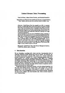
II. S TREAM P ROCESSING IN C OMPUTATIONAL S CIENCE Fig. 1.

Stream processing in computational science introduces challenges not always fully present in domains such as finance, media streaming, and business (such as RFID tags). We characterize the list of unique requirements to data driven computational science as follows. We argue that the most data driven applications we have observed have these requirements. A) Heterogeneous data formats. Science applications use and generate data in many different data formats, including netCDF, HDF5, FITS, JPG, XML, and ASCII. The binary formats can have complex access and retrieval APIs. B) Asynchronous streams. Stream generation rates can be highly asynchronous. One event stream might generate an event once every millisecond, while another might generate an event only once every 12 hours. Some SPEs fuse or join streams based on the assumption of relatively synchronous streams. C) Wide variance in event sizes. Events generated by a sensor are only a few bytes in size while events generated by large-scale instruments or regularly run models can be in the 10’s of megabytes in size. D) Timeliness is relative. One application may want to be notified the instant a condition occurs, whereas for a second application a condition may only emerge over days or weeks. E) Streaming is part of larger system. Stream processing in data-driven computational science can be one small part of a much larger system. Its architecture must be compatible with the overall system architecture.

Data sources around New Orleans.

F) Scientists need changes as an experiment progresses. One could envision a dynamic weather prediction workflow that data mines a region of the atmosphere looking for tornado signatures then kicks off a prediction model. The region over which data mining is carried out will change as a storm moves across the Midwest for instance. As the storm moves, the filtering criteria (e.g., spatial region) must adapt. G) Domain specific processing. Much stream processing in computational science is domain specific. For instance, a mesoscale detection algorithm classifies vortices detected in Doppler radar data. Thus, a stream processing system needs to be extensible, that is, it needs to provide mechanisms for scientists to extend stream and query processing with their own operators. III. M ETEOROLOGY E XAMPLE Meteorology is a rich application domain for illustrating the uniqueness of stream processing in scientific domains. Atmospheric scientists have considerable number and variety of weather observational instruments available to them due in large part to over 100 years of history in observing the atmosphere. Tools such as the Unidata Internet Data Dissemination (IDD) [19] system distribute many of the data products to interested universities for research purposes. The data products range considerably in their sizes and generation

rates. Table I lists nine of the most common data products. These products are moved to the location where the weather forecast model is to run, then ingested into the model at runtime. To illustrate the use of stream processing engines in this context, suppose that an atmospheric science student is studying Fall severe weather in the region around New Orleans, Louisiana (see Figure 1) and wants to kick off a regional 1km forecast when a storm cell emerges. The Figure 1 shows the region around New Orleans (approximately at 29.98 degree North Latitude and 90.25 degree West Longitude). The innerbox in Figure 1 marks an area of 2 degree Latitude height and 2 degree Longitude width around New Orleans, where one degree latitude is 70 statute miles and one degree longitude 60 is statute miles approximately. The figure is taken from the GeoGUI in LEAD portal [20]. The number of data products, their sizes and rates for the sensors that overlap the 80 mile radius around New Orleans are given in Table I. We call this the New Orleans Workload. The table shows nine data products, and for each type gives the number of sources. The event rate is the rate at which events are generated at the source. The cumulative rate and bandwidth are calculated over all data sources within a data type and under storm mode. An event is a time stamped observation from a data source. For the NexRad Level II Doppler radar, for instance, an event corresponds to a scan, where one scan consists of fourteen 360 degree sweeps of a radar. A scan completes in 5-7 minutes. The range given in the event size column of the table is bipolar: the small event size occurs during clear skies, and the large event size occurs during storm conditions. The variability in event rates in Table I, from 0.08 ev/hr to 1 ev/min, and variability in event sizes, from 1 KB to 41 MB, clearly demonstrates several stream processing requirements of Section II, specifically asynchronous streams (requirement B), and wide variances in event sizes (requirement C). This collection of data products also demonstrates a common requirement of stream processing in scientific domains, that of heterogeneous data products (requirement A). The product formats shown in Table I alone include text, raw radar format, model specific binary format, images, and netCDF data. IV. C ALDER A RCHITECTURE Calder, developed at Indiana University, falls into the category of a stream processing engine (SPE). Its purpose is to provide timely access to data streams. Additional details of the system architecture can be found in [13]. In this section, we provide a brief overview of the system architecture and show how a stream processing fits into a larger datadriven computational science application. In particular, we discuss a scenario in the context of the mesoscale meteorology forecasting example of Section III. We view data streams as a virtual data repository, that while

service factory continuous query dynamic deployment

handlers for incoming channels query

Pub−sub System

continuous query

query

GDS

planner

GDS

service

GDS

query

point of presence channels, one per event type

query rowset request

runtime container

response chunk

query execution engine

rowset service − ring buffers hold results

data sources

Calder System

Fig. 2.

Calder architecture.

constantly changing, has many similarities to a database [21]. Like a database, a collection of streams is bound by coherence, in that the streams belonging to a collection are related to one another, and possess meaning in that a collection of streams can be described. We call such a collection of streams a Virtual Stream Store. Calder manages multiple virtual stream stores simultaneously and provides users with query access to one or more virtual stream stores. Calder uses a publish-subscribe system, dQUOBEC [22] as its underlying transport layer. How sensors and instruments are pub-sub enabled is outside our scope of research, but solutions exist, such as [23], which takes an XML approach. This pubsub enabling is shown in Figure 2 as a single point of presence, however other approaches exist. In the simplified diagram of Figure 2, the data streams flow to a query execution engine where they are received by handlers. The runtime acts on each incoming event by triggering one or more queries. A query executes on the event, and generates zero, one, or more events that either trigger other queries in the system or flow to the Rowset Service where they are stored to a ring buffer for user access. User interaction with Calder follows the Globus OGSI model of service interaction where a grid data service (GDS) is created on behalf of a user to serve an interaction with the virtual stream store. The user submits SQL-like queries through the GDS. Details of the extended GDS interface are given in [24]. The query planner service optimizes and distributes queries and query fragments based on local and global optimization criteria. The query planner service initiates a request to the rowset service to create a new ringbuffer for the query. Calder supports monotonic time-sequenced SQL SelectFrom-Where queries. The operators supported are select/project/join operators where the join operator is an equijoin over the logical or physical time fields; the boolean operations are AND and OR; and relational operations are








































































/



#

$

%

&

'

(

'

)

*

+











0













$





$

,

(



1







































'

6







$

3

#

5

&

)

4

$