Martha Argerich, Jorge Bolet, Shura Cherkassky, Alfred Cortot, Alicia de. Larocha, and Maurizio Polini. We also set the time weighting factor α to. 1000 and the ...
Stream Segregation Algorithm for Pattern Matching in Polyphonic Music Databases Wai Man Szeto and Man Hon Wong Department of Computer Science and Engineering The Chinese University of Hong Kong Shatin, N.T., Hong Kong {wmszeto, mhwong}@cse.cuhk.edu.hk Keywords: Multimedia databases, music information retrieval, clustering algorithms
Abstract As music can be represented symbolically, most of the existing methods extend some string matching algorithms to retrieve musical patterns in a music database. However, not all retrieved patterns are perceptually significant because some of them are, in fact, inaudible. Music is perceived in groupings of musical notes called streams. The process of grouping musical notes into streams is called stream segregation. Stream-crossing musical patterns are perceptually insignificant and should be pruned from the retrieval results. This can be done if all musical notes in a music database are segregated into streams and musical patterns are retrieved from the streams. Findings in auditory psychology are utilized in this paper, in which stream segregation is modelled as a clustering process and an adapted single-link clustering algorithm is proposed. Supported by experiments on real music data, streams are identified by the proposed algorithm with considerable accuracy.
1
Introduction
As music can be represented in a series of musical notes, most of the existing methods extend some string matching algorithms to retrieve musical patterns 1
in a music database [6, 4, 5, 11, 26, 12, 10, 21, 18, 17], in which musical pitches (certain frequencies) are encoded in a finite alphabet set Σ and each alphabet is represented by an integer. Music databases can be classified according to the types of music stored: monophonic and polyphonic. If only one pitch is played at a time throughout the music, the music is said to be monophonic. If the duration of each musical note is omitted and only the sounding order of pitches is retained, monophonic music can be represented as a pitch sequence P = hp1 , p2 , . . . , pm i where pi is a pitch in the alphabet set Σ. If several pitches may be played simultaneously, the music is said to be polyphonic. The simultaneous pitches are put into a pitch set. Polyphonic music can be represented as a sequence of pitch sets, denoted by S = hS1 , S2 , . . . , Sn i where Si = {si,1 , si,2 , . . . , si,li } and si,j ∈ Σ. In other words, in the first time interval, the pitches in S1 are played. In the next time interval, the pitches in S2 are played and so on. In fact, according to this definition, most music is polyphonic. In general, recent contributions on pattern matching in polyphonic music databases mostly focus on the problem below: Given a monophonic query sequence Q = hq1 , q2 , . . . , qm i and a polyphonic source sequence S = hS1 , S2 , . . . , Sn i, the aim is to search for source subsequences hSi , Si+1 , . . . , Si+m−1 i that matches Q such that qk ∈ Si+k−1 for k = 1, 2, . . . , m. In addition to this exact matching of a query sequence, some researchers also consider vertical shifting (transposition) and edit distance [26, 11, 12, 10]. However, not all matched patterns are perceptually significant, i.e. the patterns are inaudible. In particular, the repetitive musical pattern discovery algorithm in [19] discovers over 70000 patterns in Sergei Rachmaninoff’s Prelude in C sharp minor, Op. 3 No. 2 (about-4-minute piano piece). However, the authors report that probably less than 100 of these are perceptually significant. Perceptually insignificant patterns are retrieved because music perception has not receive the attention it deserves in many existing retrieval systems. When listening to music, people perceive music in groupings of musical notes called streams which are the perceptual impression of connected series of musical notes, instead of isolated sounds. The process of grouping musical notes into streams is called stream segregation 1 . For example, a melody is usually perceived as a single coherent and continuous musical line, that is, a stream. Monophonic musical patterns across streams are perceptually insignificant and should be pruned from searching results. Consider the opening theme of 1
In [2], stream segregation is divided into two processes: simultaneous integration and sequential integration. Simultaneous integration is the process of grouping frequencies into musical notes. Sequential integration is the process of grouping musical notes into streams. However, in this paper, stream segregation is referred to the latter process only.
2
Ludwig van Beethoven’s Symphony No. 5, i.e. G, G, G, E[, F, F, F, and D (or mi, mi, mi, doh, ray, ray, ray, and te) as shown in Figure 1, if we search for any of its transposition, a matched pattern is found in the bars 1 to 2 of Frederic Chopin’s Prelude No. 4 in E minor (Figure 2). However, this pattern is hardly audible because as shown in Figure 2, there are four streams or musical lines in the opening [23]. We perceive stream 1 as the melody, while the other three streams are combined and formed a single accompaniment. The pattern is across streams 3 and 4 so it is perceptually insignificant2 .
C
A#
Pitch
G#
F#
E
D
C
0
1
2
3
4
5
6
7
8
9
10
Sequence index k
Figure 1: The opening of Beethoven’s Symphony No. 5, first movement and its monophonic sequence representation Q = hqk i for k = 1, . . . , 8. Pruning stream-crossing monophonic patterns can be done if all streams in a music database are segregated and musical patterns are retrieved from the streams. Therefore, stream segregation should be added as a pre-processing step in existing retrieval systems in order to improve the quality of retrieval. Findings in auditory psychology are utilized in this paper, in which stream segregation is modelled as a clustering process and an adapted single-link clustering algorithm is proposed. The rest of the paper is organized as follows. Section 2 provides the psychological perspective of stream segregation. Related work is reviewed in Section 3. We will present our method in Section 4. The application of stream segregation to polyphonic music databases 2
The musical excerpts can be heard at the http://www.cse.cuhk.edu.hk/˜wmszeto/stream/index.html.
3
demonstration
web
site
F# E D
Stream 1
C A# G#
Pitch
F# E
Stream 2 D C A#
Stream 3 G#
Stream 4
F# E D
0
5
10
15
20
25
Sequence index i
Figure 2: The opening of Chopin’s Prelude No. 4 in E minor and its monophonic sequence representation S = hSi i for i = 1, . . . , 18. The circles in the staff and the solid line in the sequence representation correspond to the Beethoven’s symphony.
is discussed in Section 5. In Section 6, we show our experimental results. Finally, a conclusion is given in Section 7.
2
Findings in auditory psychology
Extensive psychological experiments have been being designed to study the factors of stream segregation. The following findings are summarized from the surveys and the findings in [24, 2, 27, 7]. Most studies of stream segregation in psychology are influenced by the “Gestalt principles of perception” proposed in the 1920s. It is a set of principles governing the grouping of elements in perception. One of the principles is proximity: closer elements are grouped together in preference to those that are spaced further apart. It has been found that the pitch proximity and the temporal proximity are dominant factors in stream segregation. Pitch proximity states that musical notes which are closer in terms of pitch are grouped together. When a sequence of two alternating pitches A and B is played as ABAB . . ., the two pitches will seem to fuse into a single stream ABAB . . . if they are close together in pitch (Figure 3(a)); otherwise they will seem to form two independent streams AA . . . and BB . . . (Figure 3(b)). For temporal proximity, 4
it states that musical notes which are closer in terms of time are grouped together. When a sequence of two alternating pitches is played, we tend to perceive them as a single stream if the alternation speed is low (Figure 4(a)). If the alternation speed is high, the two pitches will form two independent streams (Figure 4(b)). Although timbre, amplitude, and spatial location may sometimes affect stream segregation, they are often outweighed by pitch and temporal proximities. (a)
(b)
B
B
A
B
A
B
B
Frequency
Frequency
B
A
A
A
Time
A
Time
Figure 3: Illustrations of the pitch proximity (adapted from [2, 27]).
(b)
B
B
A
Frequency
Frequency
(a)
A
Time
B A
B A
B A
B A
B A
B A
B A
Time
Figure 4: Illustrations of the temporal proximity (adapted from [2, 27]). In fact, there are three basic assumptions in many psychological experiments of stream segregation [24]. The first assumption is that listeners tend to assign a musical note to only one stream. A musical note would not belong to more than one stream. The second assumption is that for a given stream, there will not be more than one musical note at the same time. A stream would not contain any simultaneous musical notes. Hence, streams are monophonic. The third assumption states that there is a preference to perceive fewer streams. We tend to minimize the number of streams. 5
3
Related work
Various methods have been proposed for stream segregation and some of which are reviewed in [24]. Based on an analogy with the apparent motion in vision, Gjerdingen proposes a massively parallel, multiplex, feed-forward neural-network system in [8]. In the system, the input is musical notes which are discrete events represented in a pitch-time plane. The “influence” of an event is measured as activation. An event has greatest activation at its pitch value and during its time span. Its influence also “diffuses” to surroundings. A temporal filter smooths the activations of all events in the time dimension. A spatial filter diffuses events over a wider span of pitches with the assumption of a Gaussian distribution of the diffusion. The hill-like activation of all events are summed up. Tracking local maxima of activation along the time dimension can produce a pitch-time graph containing lines, which are interpreted as streams. The model can also track more than one line simultaneously. However, the lines in the pitch-time graph may be difficult to interpret. The McCabe and Denham’s model in [16] is similar to Gjerdingen’s. Like Gjerdingen’s model, the McCabe-Denham model represents music in the dimensions of pitch and time and uses neural networks to find out streams. There are two neural networks. One neural network corresponds to the “foreground” stream and another corresponds to the “background” stream. Musical input is segregated into the two streams. Although the McCabeDenham model accepts acoustic input, complex acoustic signals have not been tested. Similar to Gjerdingen’s model, the graphical output of McCabeDenham model may be difficult to interpret. Moreover, it can track only two streams. The latest model, developed by Temperley [24], is based on a set of stream segregation preference rules adapted from Lerdahl and Jackendoff [13], and is built on a rule-based stream segregation model in [14]. Its input is discrete pitch events. Pitches are in the unit of MIDI pitch number, which is one of the integers ranging from 0 to 127 inclusively. Middle C is assigned with the value 60. The time dimension is quantized. Hence, music is represented in a pitch-time grid of squares. If there is a note, the square is “black”. If not, the square is “white”. The model has six mandatory preference rules and one optional preference rule. A user is required to input the weight of each rule and the maximum number of streams. Then the system searches for the optimal stream configuration using dynamic programming. However, overlapping notes of the same pitch are disallowed in the input representation and there is no known experimental evidence to show that MIDI pitch number is an appropriate perceptual distance. 6
4
Proposed method
According to the findings in auditory psychology discussed in Section 2, there are four important preferences in stream segregation: (i) the pitch proximity and the temporal proximity are dominant factors; (ii) a musical note is assigned to only one stream but not more; (iii) a stream does not contain any simultaneous musical notes; and (iv) the number of streams is minimized. Based on these findings, we represent music as events and propose a clustering model for stream segregation.
4.1
Music representation
As pitch and temporal proximities are dominant, the attributes of pitch and time of music are taken into account. Each musical note is represented as an event. An event e is a vector (ts , te , p), where ts is the start time, te is the end time, and p is the pitch. The start time and the end time are in the unit of seconds. The pitch is represented as the frequency in the mel scale [20, 3]. The mel scale represents the average judgement of the relation between perceptual pitch and frequency, where the scale is adjusted such that 1000 mels map to 1 kHz. The mapping is approximately linear in frequency up to 1 kHz, and logarithmic beyond 1 kHz. The scale is defined in the following analytical expression: fmel = 2595 · log10 (1 +
fHz ) 700
An example is shown in Figure 5 and Table 1. ei Pitch name (ts , te , p) e1 C4 (0, 2, 357.87) e2 G4 (0, 0.5, 501.15) e3 A[4 (1, 3, 524.96) e4 E4 (2, 4, 434.88) e5 F4 (3, 4, 456.13) Table 1: The events in the five-event example.
4.2
Algorithm
Intuitively, if musical notes are represented as events in the pitch-time space, the “distance” between two events can reflect the pitch proximity and the temporal proximity of the corresponding musical notes. A stream, a group of 7
600
550
e3 e2
Frequency (mel)
500
e
5
450
e
4
400
350
e
1
300
0
0.5
1
1.5
2
2.5
3
3.5
4
4.5
Time (second)
Figure 5: A five-event example. The speed is 60 crotchet beats per minute.
events sharing “similar” pitch attribute and time attribute, is in fact a cluster, so stream segregation can be modelled as a clustering problem. A stream is thus referred to as a cluster hereinbelow. However, traditional clustering techniques cannot be directly applied to stream segregation because they handle data points rather than events. Moreover, besides the pitch and the temporal proximities, the findings in auditory psychology show that there are preferences to include each event in only a single stream and to avoid multiple simultaneous events in a single stream. To include these findings, we define two kinds of the relation between two events: sequential events and simultaneous events. Given two events, if their durations overlap each other, they are simultaneous events. Otherwise, they are sequential events. The definitions are formally given below: Definition 4.1 (Sequential events) Given two events e1 = (ts1 , te1 , p1 ) and e2 = (ts1 , te2 , p2 ), they are sequential events if te1 ≤ ts2 or te2 ≤ ts1 , denoted by e1 ∦ e2 . If te1 ≤ ts2 , then e1 ≺ e2 . If te2 ≤ ts1 , then e1 Â e2 . Definition 4.2 (Simultaneous events) If two events e1 and e2 are not sequential events, they are said to be simultaneous events, denoted by e1 k e2 . These definitions are further illustrated by the following example: Example 4.1 In Figure 5, the event pairs {e1 , e4 }, {e1 , e5 }, {e2 , e3 }, {e2 , e4 }, {e2 , e5 }, and {e3 , e5 } are sequential events because they do not overlap each other in time. The event pairs {e1 , e2 }, {e1 , e3 }, {e3 , e4 }, and {e4 , e5 } are simultaneous events. 8
After defining the relations between events, we define the distance function between two events. To avoid putting simultaneous events in the same cluster, the distance between any two simultaneous events is set to infinity. Hence, a cluster cannot contain any simultaneous event. For sequential events, it is the distance between the tail of the prior event and the head of the posterior event. In order to define the concept formally, we need to address two problems. The first one is the choice of metrics. However, a definitive answer to the most appropriate choice of metrics to “musical” space, to our knowledge, has never been done. Therefore, we use the Euclidean distance, the most common metric. The second problem is the difference of measurement units of pitch and time. We tackle it by assigning weighting factors to the time dimension and the pitch dimension. The weighting factors will be determined empirically. The inter-event distance function is defined below: Definition 4.3 (Inter-event distance) Given two events e1 = (ts1 , te1 , p1 ) and e2 = (ts1 , te2 , p2 ), the inter-event distance EDIST is (p (αd)2 + (β(p1 − p2 ))2 if e1 ∦ e2 , EDIST (e1 , e2 ) = ∞ if e1 k e2 . where α is the time weighting factor, β is the pitch weighting factor, and ( te − ts2 if e1 ≺ e2 , d = 1e t2 − ts1 if e1 Â e2 . Example 4.2 Suppose α = 1 and β = 1. The inter-event distances between all possible pairs of the events in Figure 5 are shown in Table 2 3 . e1 e2 e3 e4 e5 e1 − ∞ ∞ 77.11 98.39 e2 ∞ − 23.83 66.36 45.14 e3 ∞ 23.83 − ∞ 68.89 e4 77.11 66.36 ∞ − ∞ e5 98.39 45.14 68.89 ∞ − Table 2: The inter-event distances of the events in Figure 5 (α = 1; β = 1). Before going further, we define some notations adapted from those of the traditional clustering techniques in [25]. A piece of music E consists of N 3
The self-distance of events is not shown and is marked in “−” because an event does not form a cluster with itself.
9
events: E = {ei | i = 1, 2, . . . , N } A cluster C has the start time T s , the end time T e , and a set of clustered events C: C = (T s , T e , C) where C = {ei1 , ei2 , . . .} ⊆ E where eik = (tsik , teik , pik ), T s = min(tsik ), ik
e
T = max(teik ). ik
A clustering R contains n clusters: R = {Cj | j = 1, 2, . . . , n} As streams have chain-like shapes, we adapt the single-link clustering algorithm for solving the stream segregation problem. An event is regarded as a data point. The single-link clustering algorithm is a hierarchical clustering method, which generates a nested series of partitions of data points. In the single-link method, the distance between two clusters is the minimum of the distances among all pairs of data points drawn from the two clusters (one data point from the first cluster, the other from the second) [9]. In order to avoid a cluster containing any simultaneous events, we define the following two relations between two clusters similar to those between two events. Definition 4.4 (Sequential clusters) Given two clusters C1 = (T1s , T1e , C1 ) and C2 = (T2s , T2e , C2 ), they are sequential clusters if T1e ≤ T2s or T2e ≤ T1s , denoted by C1 ∦ C2 . Definition 4.5 (Simultaneous clusters) If two clusters C1 and C2 are not sequential clusters, they are said to be simultaneous clusters, denoted by C1 k C2 . The inter-cluster distance between simultaneous clusters should be set to infinity to ensure that no pair of simultaneous events is in the same cluster. For two sequential clusters, the distance between them is the minimum of the distances among all pairs of events drawn from one cluster and another cluster. We define the inter-cluster distance below: 10
Definition 4.6 (Inter-cluster distance) Given two clusters C1 = (T1s , T1e , C1 ), C2 = (T2s , T2e , C2 ), the inter-cluster distance CDIST is ( CDIST (C1 , C2 ) =
minei ∈C1 ,ej ∈C2 (EDIST (ei , ej )) ∞
if C1 ∦ C2 , if C1 k C2 .
There are various methods to implement the single-link clustering algorithm. Here, we adapt the agglomerative algorithm in [25, 15, 9]. For the agglomerative algorithm, the initial clustering R0 consists of N clusters, each of which contains one event in E. Among all possible pairs of clusters, find the pair that has the minimum inter-cluster distance over all other pairs. Then the pair of clusters is merged into a larger cluster. Thus, a new clustering R1 is formed and the process is repeated. Following the psychological preference that the number of streams is minimized, we minimize the number of clusters by setting the two termination conditions as follows. The first condition is that the distances of all possible pairs of clusters are infinity. This means that all pairs of clusters are simultaneous clusters. Noted that during the clustering process, only sequential clusters but not simultaneous clusters can be merged together. Hence, the resulting clusters will not contain any simultaneous events. The second condition is that all events lie in the same cluster, i.e. one large cluster contains all events, in which any two events must be sequential events. As a result, users are not required to input the threshold or the number of clusters. The adapted single-link clustering is shown in Algorithm 1. Algorithm 1 Adapted single-link clustering algorithm 1: Choose R0 ← {Ci = (tsi , tei , {ei }), i = 1, 2, . . . , N } as the initial clustering. 2: t ← 0 3: repeat 4: t←t+1 5: Among all possible pairs of clusters (Cr , Cs ) in Rt−1 , find Ci , Cj such that CDIST (Ci , Cj ) = minr6=s CDIST (Cr , Cs ) if CDIST (Ci , Cj ) = ∞ then 6: 7: break 8: Merge Ci , Cj into a single cluster Cq and form Rt ← (Rt−1 − {Ci , Cj }) ∪ Cq . 9: until RN −1 clustering is formed, i.e., all events lie in the same cluster. Generated by the algorithm running on the example in Figure 5 with α = 1 and β = 1, the iterative clustering results are shown in Table 3. The 11
clustering of the five-event example is presented in Figure 6, where {e1 , e4 } is a cluster and {e2 , e3 , e5 } is another. {e1 } {e1 } − {e2 } ∞ {e3 } ∞ {e4 } 77.11 {e5 } 98.39 (a) t = 0
{e2 } {e3 } {e4 } ∞ ∞ 77.11 − 23.83 66.36 23.83 − ∞ 66.36 ∞ − 45.14 68.89 ∞
{e5 } 98.39 45.14 68.89 ∞ −
{e1 } {e2 , e3 } {e4 } {e5 } {e1 } − ∞ 77.11 98.39 {e2 , e3 } ∞ − ∞ 45.14 {e4 } 77.11 ∞ − ∞ {e5 } 98.39 45.14 ∞ − (b) t = 1
{e1 } {e2 , e3 , e5 } {e4 } {e1 } − ∞ 77.11 {e2 , e3 , e5 } ∞ − ∞ {e4 } 77.11 ∞ − (c) t = 2
{e1 , e4 } {e2 , e3 , e5 } {e1 , e4 } − ∞ {e2 , e3 , e5 } ∞ − (d) t = 3
Table 3: Inter-cluster distance and clustering at different t of the five-event example.
600
550
e3 e
2
Frequency (mel)
500
e
5
450
e4
400
350
e1 300
0
0.5
1
1.5
2
2.5
3
3.5
4
4.5
Time (second)
Figure 6: Clustering result: {e1 , e4 } is a cluster and {e2 , e3 , e5 } is another. Motivated by the analysis of the general single-link method in [25], the complexity of the adapted algorithm is analyzed as follows. At each level t, there are N − t clusters. Thus, in order to determine the pair of clusters that is going to be merged at the (t + 1)th level, the number of pairs of clusters
12
to be considered is
µ
¶ N −t (N − t)(N − t − 1) = . 2 2
Therefore, if the number of output clusters is n, the total number of pairs that have to be examined throughout the whole clustering process is ¶ N µ ¶ N −n µ X X k N −t = 2 2 t=0 k=n N µ ¶ n−1 µ ¶ X X k k = − 2 2 k=0 k=0 (N − 1)N (N + 1) 6 (n − 2)(n − 1)n − 6 As n is small comparing to N , the total number of operations is proportional to N 3 . The calculation of the inter-event distance takes constant time. Therefore, the complexity of the algorithm is O(N 3 ). =
5
Application of Stream Segregation to Polyphonic Databases
Recapitulating the exact musical pattern matching problem stated in Section 1 that given a monophonic pitch query sequence Q = hq1 , q2 , . . . , qm i and a polyphonic pitch-set source sequence S = hS1 , S2 , . . . , Sn i where Si = {si,1 , si,2 , . . . , si,li } and qi , si,j are in the finite alphabet set Σ, the aim is to search for source subsequences hSi , Si+1 , . . . , Si+m−1 i that matches Q such that qk ∈ Si+k−1 for k = 1, 2, . . . , m. In order to avoid retrieving perceptually insignificant patterns, we propose that stream segregation is added as the pre-processing step in a retrieval system, i.e., all polyphonic sources are segregated into streams and the streams are stored in a database. Then patterns are retrieved from the streams. As streams are monophonic, stream segregation actually reduces a polyphonic music database to a monophonic one. The pitches of streams are extracted to form pitch source sequences. The ordering of pitches follows their appearance order. Example 5.1 In Figure 6, {e1 , e4 } is a stream and {e2 , e3 , e5 } is another stream. The pitch of ei is pi where pi ∈ Σ. As e1 ≺ e4 and e2 ≺ e3 ≺ e5 , the two streams become two pitch source sequences hp1 , p4 i and hp2 , p3 , p5 i. 13
Then the exact musical pattern matching problem is redefined as follows: Given a pitch query sequence Q = hq1 , q2 , . . . , qm i and a pitch source sequence S = hs1 , s2 , . . . , sn i where qi , si ∈ Σ, the aim is to search for source subsequences hsi , si+1 , . . . , si+m−1 i that matches Q such that qk = si+k−1 for k = 1, 2, . . . , m. This is like a substring matching problem. Moreover, no matched pattern is across streams so the opening theme of Beethoven’s Symphony No. 5 cannot be found in Chopin’s Prelude No. 4 in E minor (Figure 2) if the streams of Chopin’s Prelude are correctly segregated. The correctness of stream segregation greatly affects the accuracy of the stream-segregated retrieval system. If an event is wrongly classified into a stream, matched patterns may be missed and false alarms may occur. Hit rate and false alarm rate are proposed to evaluate the quality of stream segregation. Before introducing them, we place a total ordering on events for a simpler notation in later discussions. Events are first sorted by the start time in the ascending order. If two events have the same start time, the order is determined arbitrarily. The index i of the event ei reflects this total ordering: given a music E = {e1 , e2 , . . . , eN }, the total ordering is e1 < e2 < · · · < eN . For example, the index of each event in the five-event example in Figure 5 has been assigned according to the total ordering such that e1 < e2 < e3 < e4 < e5 . The correctness of stream segregation is measured in terms of linkage between two events. Given a stream C = {ei1 , ei2 , . . . , eik } where i1 < i2 < · · · < ik , there exists linkages in the pairs (ei1 , ei2 ), (ei2 , ei3 ), . . . , (eik−1 , eik ). The pitch of eir is pir then the corresponding pitch source sequence is hpi1 , pi2 , . . . , pik i. Example 5.2 In Figure 6, {e1 , e4 } and {e2 , e3 , e5 } are the streams. Their linkages are {(e1 , e4 ), (e2 , e3 ), (e3 , e5 )}. Hit rate and false alarm rate are used to evaluate the stream segregation result of the music in which the natural streams are known. Natural streams, a term borrowed from natural clusters, are pre-defined streams of the music. In other words, the “correct” stream segregation result have already been known. Streams segregated by our algorithm are called output streams, which are compared to the natural streams. A hit is a linkage of an event pair that exists in both the natural stream and the output stream. A false alarm is a linkage that exists in an output stream but not any natural streams. The hit rate and the false alarm rate are defined as follows. Definition 5.1 (Hit rate) H=
Number of hits Number of linkages in natural streams 14
Definition 5.2 (False alarm rate) A=
Number of false alarms Number of linkages in output streams
Example 5.3 Suppose the natural streams in the five-event example in Figure 5 are {e1 , e4 }, {e2 , e5 }, and {e3 } so the linkages are {(e1 , e4 ), (e2 , e5 )}. The linkages of the output streams are {(e1 , e4 ), (e2 , e3 ), (e3 , e5 )} as in Example 5.2. The hit rate H = 1/2 = 0.5 and the false alarm rate A = 2/3 = 0.667. Suppose that a subsequence S 0 matches the query Q. If it is a correct match, all linkages of the corresponding events in S 0 must be hits; otherwise, the subsequence S 0 is missed. If the match is a false alarm, at least one linkage of the corresponding events in S 0 is a false alarm. Assuming that the probability of a hit is independent from the previous hits and the probability of a false alarm is independent from the previous false alarms, we define the probabilities of a hit and of a false alarm for an m-length query in Definitions 5.3 and 5.4 respectively. Definition 5.3 (Probability of a hit for an m-length query) Hm = (H)m−1 for m ≥ 2 Definition 5.4 (Probability of a false alarm for an m-length query) Am = 1 − (1 − A)m−1 for m ≥ 2 The probability of a hit for an m-length query is the probability not to miss an m-length query; while the probability of a false alarm for an m-length query is the probability of a matched pattern for an m-length query being a false alarm. In the next section, experiments are performed to verify our proposed solution.
6
Experimental Results
We implement our distance functions and adapt the implementation of the single-link clustering algorithm in [15] for demonstrating the capability and usefulness of our proposed method. We collect real polyphonic music data in the MIDI (Musical Instrument Digital Interface) format, which is the most popular encoding scheme to represent music symbolically. 15
In the first experiment, we adjust the time weighting factor α and set the pitch weighting factor β to 1 to investigate their effect on the hit rate and the false alarm rate. The MIDI file of Johann Sebastian Bach’s two-part Invention No. 1 is collected from [22]. The opening six bars of Invention No. 1 are shown in Figure 7. A two-part Invention is a two-voice keyboard piece, in which the upper voice is played by the right hand and the other by the left. On the facsimile of the title page of the autograph of 1723, Bach wrote that a two-part Invention should be “learned to play cleanly in two parts” [1]. Except the final bar in Invention Nos. 1 and 8, there is at most two musical notes at a time. Thus, the two parts in an Invention are considered as two natural streams in our experiment. The final bars of the Invention Nos. 1 and 8 are removed (No. 8 will be used in the second experiment). In all streams, each musical note has a linkage to its adjacent musical notes. We compare the output streams generated by our method with the natural streams. The speed of Invention No. 1 is the average value over 2 editions, 2 commentaries, and 9 recordings from [1].
Figure 7: The opening six bars of Bach’s Invention No. 1. The hit rate and the false alarm rate against the time weighting factor are shown in Figures 8(a) and 8(b) respectively. When the time weighting factor increases, the hit rate increases and the false alarm rate decreases and then both of them become stable at 0.991 and 0.009 respectively. In the stable range, we choose the time weighting factor 1000 and the pitch weighting factor 1 arbitrarily and verify these values in the next two experiments. Meanwhile, the clustering result of Invention No. 1 for the time weighting factor 1000 and the pitch weighting factor 1 is depicted in Figure ??.
16
0.1 0.09
0.98
0.08
0.97
0.07 False alarm rate
1 0.99
Hit rate
0.96 0.95 0.94
0.06 0.05 0.04
0.93
0.03
0.92
0.02
0.91
0.01
0.9 0
200
400
600
800 1000 1200 1400 Time weighting factor α
1600
1800
0 0
2000
200
400
600
800 1000 1200 1400 Time weighting factor α
(a)
1600
1800
2000
(b)
Figure 8: Experiment 1. (a) The hit rate against the time weighting factor α of Bach’s Invention No.1. (b) The false alarm rate against the time weighting factor α of Bach’s Invention No.1. 1000
900
800
Frequency (mel)
700
600
500
400
300
200
100 0
0.5
1
1.5
Weighted time
2
2.5
3 4
x 10
Figure 9: Clustering result of the opening six bars of Invention No. 1 (α = 1000; β = 1). The two continuous lines are the output streams which are the same as the natural streams. The vertical lines are the bar-lines. In the second experiment, we test our method on all 15 Bach’s two-part Inventions collected from [22]. The speed of each Invention is the average value from [1]. We set the time weighting factor α to 1000 and the pitch weighting factor β to 1. In Figure 10, the hit rate and the false alarm rate of the 15 Bach’s two-part Inventions are plotted. The average hit rate and the average false alarm rate of the 15 Inventions are 0.986 and 0.015 respectively. The average probabilities of a hit and of a false alarm against the query length are shown in Figure 11. When the length of a query increases, the average 17
probability of a hit decreases linearly while the average probability of a false alarm increases gradually linearly. 1
0.9
Hit rate False alarm rate
0.8
0.7
0.6
0.5
0.4
0.3
0.2
0.1
0
0
2
4
6
8
10
12
14
16
Invention number
Figure 10: The hit rate and the false alarm rate of the 15 Bach’s two-part Inventions
1
0.8
Average probability of a hit for a query Average probability of a false alarm for a query
0.6
0.4
0.2
0
1
2
3
4
5
6
7
8
9
10
11
Query length
Figure 11: The average probabilities of a hit and a false alarm of the 15 Bach’s two-part Inventions against the query length In the third experiment, we tested whether our method can find the correct linkages of the four streams in the opening two bars of Chopin’s Prelude No. 4 in E minor, the piano piece discussed in Section 1. The natural streams are the four streams shown in Figure 2. In all streams, each musical note has a linkage to its adjacent musical notes. The speed is 64.5 crotchet beats per minute, the average value of 6 performances including 18
Martha Argerich, Jorge Bolet, Shura Cherkassky, Alfred Cortot, Alicia de Larocha, and Maurizio Polini. We also set the time weighting factor α to 1000 and the pitch weighting factor β to 1 as in our previous experiments. The clustering result are depicted in Figure 12. Only four output streams are generated. The hit rate and the false alarm rate are 1 and 0 respectively. No event is misclassified. The probabilities of a hit and of a false alarm against the query length are shown in Figure 13. 700
650
600
Frequency (mel)
550
500
450
400
350
300
250 3000
4000
5000
6000
7000
8000
9000
10000
11000
12000
13000
14000
Weighted time
Figure 12: Clustering result of the opening two bars of Chopin’s Prelude in E minor (α = 1000; β = 1). The four continuous lines are the output streams which are the same as the natural streams in Figure 2. The vertical lines are the bar-lines.
1 Probability of a hit for a query Probability of a false alarm for a query 0.8
0.6
0.4
0.2
0
1
2
3
4
5
6
7
8
9
10
11
Query length
Figure 13: The probabilities of a hit and a false alarm of the opening two bars of Chopin’s Prelude in E minor against the query length.
19
In the fourth experiment, we evaluate the running-time performance of the adapted single-link clustering algorithm. Bach’s Invention No. 1 is divided into different lengths. We run our Matlab 6.5 implementation of the adapted single-link algorithm in a Pentium 4 PC with 512MB RAM in Microsoft Windows 2000. The CPU time against the number of events is plotted in Figure 14. Increase in the number of events relates an increase in the CPU time. Although the time complexity of the algorithm is O(N 3 ), clustering the complete Invention No.1 spends less than 12 seconds. 14
12
CPU time (second)
10
8
6
4
2
0
0
50
100
150
200
250
300
350
400
450
500
Number of events
Figure 14: CPU time vs number of events.
7
Conclusion
It is essential to incorporate stream segregation in existing music information retrieval systems in order to improve the quality of retrieval. In this paper, we tackle the stream segregation problem by representing music in the form of events, formulating the inter-event and the inter-cluster distance functions based on the findings in auditory psychology, and applying the distance functions in the adapted single-link clustering algorithm. Supported by the experiments on real music data, our proposed method can successfully identify streams with a high hit rate and a low false alarm rate.
Acknowledgements We are thankful to Dennis Wu and Eos Cheng for their valuable comments.
20
References [1] J. S. Bach. Inventions and Sinfonias (Two- and Three-Part Inventions). Alfred Publishing Co., 2nd edition, 1991. [2] A. S. Bregman. Auditory Scene Analysis: the Perceptual Organization of Sound. The MIT Press, 1990. [3] D. Butler. The musician’s guide to perception and cognition. Schirmer Books, 1992. [4] D. Byrd and T. Crawford. Problems of music information retrieval in the real world. Information Processing and Management, 38:249–272, 2002. [5] E. Cambouropoulos, T. Crawford, , and C. Iliopoulos. Pattern processing in melodic sequences: Challenges, caveats and prospects. In Proc. AISB’99 Symposium on Musical Creativity, pages 42–47, 1999. [6] T. Crawford, C.S. Iliopoulos, and R. Raman. String matching techniques for musical similarity and melodic recognition. Computing in Musicology, 11:73–100, 1998. [7] D. Deutsch, editor. The Psychology of Music. Academic Press, 2nd edition, 1999. [8] R. O. Gjerdingen. Apparent motion in music. Music Perception, 11:335– 370, 1994. [9] A. K. Jain, M. N. Murty, and P. J. Flynn. Data clustering: a review. ACM Computing Surveys, 31(3):264–323, 1999. [10] K. Lemstrom. String Matching Techniques for Music Retrieval. PhD thesis, University of Helsinki, Finland, 2000. [11] K. Lemstrom and S. Perttu. Semex - an efficient music retrieval prototype. In First International Symposium on Music Information Retrieval (ISMIR 2000), Plymouth, Massachusetts, October 23-25 2000. [12] K. Lemstrom and J. Tarhio. Searching monophonic patterns within polyphonic sources. In Proc. Content-Based Multimedia Information Access (RIAO’2000), volume 2, pages 1261–1279, Paris, France, April 12-14 2000.
21
[13] F. Lerdahl and R.S. Jackendoff. A Generative Theory of Tonal Music. The MIT Press, 1983. [14] A. Marsden. Computer Representations and Models in Music, chapter Modelling the perception of musical voices: A case study in rule-based systems, pages 239–263. Academic Press, 1992. [15] MathWorks. Statistics toolbox version 4, 2002. [16] S. L. McCabe and M. J. Denham. A model of auditory streaming. The Journal of the Acoustical Society of America, 101(3):1611–1621, March 1997. [17] R. J. McNab, L. A. Smith, I. H. Witten, and C. L. Henderson. Tune retrieval in the multimedia library. Multimedia Tools and Applications, 10(2/3):113–132, 2000. [18] M. Melucci and N. Orio. Musical information retrieval using melodic surface. In Proc. ACM International Conference on Digital Libraries, pages 152–160, 1999. [19] D. Meredith, G. A. Wiggins, and K. Lemstrom. A geometric approach to repetition discovery and pattern matching in polyphonic music. Presented at Computer Science Colloquium, Department of Computer Science, King’s College London, November 21 2001. [20] D O’Shaughnessy. Speech Communication. Addison-Wesley, 1987. [21] J. Pickens. A survey of feature selection techniques for music information retrieval, 2001. [22] Mutopia Project. Music listing: J. S. Bach’s inventions. http://www.mutopiaproject.org/cgibin/maketable.cgi?Composer=BachJS, 2001. [23] C. Schachter. Chopin Studies 2, chapter The Prelude in E minor Op. 28 No. 4: autograph sources and interpretation, pages 140–161. Cambridge University Press, 1994. [24] D. Temperley. The Cognition of Basic Musical Structures. The MIT Press, 2001. [25] S. Theodoridis and K. Koutroumbas. Pattern recognition. Academic Press, 1999. 22
[26] A. Uitdenbgerd and J. Zobel. Melodic matching techniques for large music databases. In Proc. ACM International Multimedia Conference, pages 57–66, 1999. [27] L. P. A. S. van Noorden. Temporal coherence in the perception of tone sequences. PhD thesis, Eindhoven University of Technology, 1975.
23