[8] John Jannotti, David K. Gifford, Kirk L. Johnson, Frans M. Kaashoek, and James W. ... [18] Tara Small, Baochun Li, Senior Member, and Ben Liang. Outreach:.
Streamline: An Architecture for Overlay Multicast Amirhossein Malekpour and Fernando Pedone
Mouna Allani and Benoˆıt Garbinato
University of Lugano, Switzerland {malekpoa, fernando.pedone}@unisi.ch
University of Lausanne, Switzerland {mouna.allani, benoit.garbinato}@unil.ch
Abstract—We propose Streamline, a two-layered architecture designed for media streaming in overlay networks. The first layer is a generic, customizable and lightweight protocol which is able to construct and maintain different types of meshes, exhibiting different properties. We discuss two types of overlay networks and explain how the first layer protocol builds these networks in a distributed manner. The second layer is responsible for data propagation to the nodes in the mesh by constructing an optimized diffusion tree. In order to cover the vulnerabilities of the diffusion tree, we propose a masking mechanism which enables the nodes to instantly switch to alternative data paths when necessary. Our simulations reveal that, the structure and properties of the underlying mesh are key to the performance of the system and Streamline can tolerate high node churn without degrading delivery rate. Index Terms—Peer to peer; overlay multicast; application level multicast.
I. I NTRODUCTION Many peer-to-peer applications (e.g., audio and video streaming, multi-party games) rely on some support for data multicast, where peers interested in a given data stream can join a corresponding multicast group. These networks are typically composed of one or more propagation trees or a single mesh. In these structures, nodes are computers and edges are overlay links formed by the establishment of peering relationships between the nodes. Despite the large research focus of the peer-to-peer community on these systems and a plethora of proposed solutions, many important questions remain unanswered. For example, little is known about the structural properties of existing overlay networks (e.g., BitTorrent, commercial overlay multicast solutions) and their causes and impacts on the application. Overlay multicast networks can be characterized by a set of measures and properties, an important element of which is the diffusion pattern. In tree-based systems, nodes diffuse the content to their children in a single or in multiple diffusion trees. Peer selection in these systems is based on classic measures like end-to-end delay and outgoing bandwidth. In mesh-based systems, where nodes pull (swarm) the data from their neighbors, peer selection is primarily based on the availability of content on nodes. In this work we propose to combine the two mechanisms by deploying a protocol stack. The first layer protocol (at the bottom) forms a sub-optimal mesh of nodes. The purpose of this layer is to maintain a connected structure as a This research is funded by the Swiss National Science Foundation, in the context of Project number 200020-120188.
basic building block on top of which different data-streaming protocols can be deployed. The second layer builds optimized propagation structures embedded in the mesh and takes care of transmission rate allocations and failures. Generally, such an architecture is suited for push-based diffusion patterns where a single or multiple propagation trees channel the data flow from the source to the set of receivers. In this work we mostly focus on the construction of the mesh structure; for brevity, data diffusion is based on a simple single propagation tree. The goal of our modular approach is to address some inherent problems in tree-based overlay streaming solutions, in particular the vulnerability of the diffusion tree against failures and its poor resource utilization. Moreover, our mesh construction protocol is a generic framework, decoupled from the diffusion mechanism, leaving our hands open to create different mesh types and probe the overall performance of the system with different structures. Using our mesh construction algorithm, we produce two types of meshes. While one network strives to arrange the nodes in a semi-regular graph (i.e., node connectivity is defined by a degree range), the other adapts the graph connectivity to the outgoing bandwidth of the nodes. We show in the paper that these two graph structures have distinguished characteristics and result in different tradeoffs. Our experimental evaluation of Streamline has revealed that the structure and properties of the underlying mesh have substantial effects on the performance of the system. This result suggests that the data dissemination problem can be “decomposed” and studied in parts, for example, one part focusing on distributed techniques to build meshes efficiently, and the other part focusing on sophisticated propagation structures. With respect to the mesh-construction algorithms we considered in this paper, our evaluation showed that while the overhead introduced by the first layer is negligible in both meshes, in the second layer the semi-regular mesh is more economical than the adaptive mesh. This reduced overhead comes with a cost however: the adaptive mesh has faster setup time (i.e., the time needed for a joining node to start receiving data) and higher reliability. The rest of the paper is structured as follows. Section II gives a bird’s-eye view of Streamline’s architecture. Section III and IV present the first and the second layers of the system. Section V describes our prototype and analyzes its performance. Section VI overviews related work and Section VII concludes the paper.
II. S YSTEM M ODEL AND A RCHITECTURE A. Model and assumptions We model the overlay network as a graph G = (V, E) in which V = {n1 , n2 , ...} is the set of nodes and V = {l1 , l2 , ...} ⊆ V ×V is the set of links between them. Links are bidirectional and imply a flow of data between the two ends. Nodes may crash and recover and links can lose messages. We assume that nodes do not behave maliciously (i.e., no Byzantine failures) and links do not corrupt messages. The system is partially synchronous, that is, there are known bounds on the time it takes for nodes to execute and on the time it takes for messages to be transmitted, but these bounds are only guaranteed to hold starting at some unknown time, called Global Stabilization Time (or GST) [5]. Streamline guarantees that the system will converge after GST (e.g., after timeout values can be set accurately). B. System architecture Streamline’s architecture breaks down the peer-to-peer protocol stack into two layers, one responsible for the formation of an overlay network and the other responsible for efficient data streaming on the overlay. The first layer, the Mesh Maintenance Layer, executes a simple lightweight protocol, intended for the construction and maintenance of the mesh; it is the protocol executed by nodes in order to join the overlay network and maintain their number of peers within a certain range. The protocol is based on the localized knowledge of the system at each node, a set of measurements, and a peer selection algorithm. It provides a basic service to the second layer, informing it about the establishment and termination of peering relations. The second layer, the Data Streaming Layer, is built on top of the Mesh Maintenance Layer and is responsible for information diffusion. To do so, this layer builds another structure, embedded in the underlying mesh without creating additional overlay links: links of the upper structure are a subset of the links of the underlying mesh. The protocol works in two phases: In the first phase nodes try to approximate the underlying mesh structure by continuously gossiping their current knowledge about the system. When a peer receives a new message, it updates its local knowledge of the network. Eventually the local information built by peers evolves into a global knowledge. In the second phase, the data source (i.e., the node willing to stream data) builds a propagation structure based on the mesh it has currently assessed. The Mesh Maintenance Layer uses two primitives to inform the upper layer about changes in the peering relationships: PeeringEstablished(n) is used by the first layer protocol to inform the second layer about establishment of a peering relationship with node n; PeeringTerminated(n) is called by layer one upon termination of a peering relationship with n. In summary, the Mesh Maintenance Layer deals with the question of which nodes should be chosen for peering while the Data Streaming Layer answers the question of which peers should be selected to stream data and how. In Sections III and IV we detail the two layers.
III. M ESH M AINTENANCE L AYER The Mesh Maintenance Protocol is a gossip-based protocol executed by all nodes. Nodes have a partial knowledge (local view) of the network. Periodically, each node selects a subset of its view and exchanges this set with other nodes in rounds of gossiping as detailed later. Nodes then start peering with some of the nodes in their local view. This process leads to the formation of a mesh. At the heart of this protocol is a function Select and two parameters assigned to each node: a minimum and a maximum degree for a node ni , denoted by mini and maxi , respectively. Depending on the target mesh structure, these limits might vary for each node relative to its outgoing bandwidth, or be the same for all of them, irrespective of their bandwidth. In order to understand the effects of the mesh structure on the performance of the system, we chose to study two types of graphs: Semi-Regular Mesh and Adaptive Mesh, both produced by the first layer protocol as detailed later. In the Semi-Regular Mesh, nodes have similar connectivity, falling within a predefined range. In such a graph the forwarding load is more evenly distributed among the nodes. In the Adaptive Mesh the degree distribution follows the outgoing bandwidth distribution of nodes. Such a network makes a better utilization of the available outgoing bandwidth of each node. We describe next Streamline’s generic bootstrapping and mesh maintenance protocol and in the following subsections we detail how we tune the protocol to construct each type of mesh. A. Mesh Maintenance Protocol We denote the set of active peers a node ni is directly connected to by Pi and the size of this set, the degree of ni , by δi . Ideally we would like ni to have a degree between mini and maxi (i.e., mini ≤ δi ≤ maxi ). Upon arrival of a node or due to departure of a large number of its peers, however, ni ’s connectivity may fall below mini , although it never exceeds maxi because when ni is at its maximum allowed degree, it does not accept any new peer. The partial knowledge or view node ni has about the network is denoted by Vi and modelled as a list of tuples of the form hn j , φ j , τ j , Q j i, where n j is some node ni knows about, φ j is the number of peers n j is willing to accept, calculated as φ j = min j − δ j , τ j is the local time at ni when the entry was added to Vi or updated, used to facilitate garbage collection of old entries, and Q j is a set containing identifiers of nodes who gave the information about n j to ni . Q j is used by ni to inform concerned nodes about changes in the state of n j . Every node maintains a small list of such tuples with a limited number of entries meaning that the node has a partial knowledge about a subset of active nodes. Node ni uses a Select(φ) function in order to pick a number of nodes from its partial view. The output of this function is a list of tuples of size k ≤ φ. The definition of this function varies based on the target mesh structure and is further discussed in the following sections. Algorithm 1 shows Streamline’s mesh maintenance protocol. In order to join the network a node executes the Bootstrap
1: procedure Bootstrap 2: φi ← mini 3: Vi ← 0/ 4: Pi ← 0/ 5: N ← QueryOracle() 6: MergeView(N, Oracle)
{query bootstrapping oracle}
7: periodically do 8: for all p ∈ Pi do 9: send heartbeat message to p 10: for all p ∈ Pi do 11: if no heartbeat received f rom p in the last period then 12: Pi ← Pi \ {p} 13: call PeeringTerminated(p) {inform the second layer} 14: if δi < mini then {δi is defined as the size of Pi } 15: φi ← mini − δi 16: Si = Select(φi ) 17: for all si ∈ Si do 18: send BeginPeering(φi ) to si 19: upon receive BeginPeering(φ j ) from n j do 20: if δi < maxi then 21: Pi ← Pi ∪ {n j } {update the list of peers} 22: send PeeringAccepted to n j 23: call PeeringEstablished(n j ) {inform the second layer} 24: else 25: S j ← Select(φ j ) 26: send PeeringRejected to n j {reject peering request} 27: send ReceiveView(S j ) to n j {send a subset of the view} 28: upon receive PeeringAccepted from n j do 29: Pi ← Pi ∪ {n j } {update the list of peers} 30: call PeeringEstablished(n j ) {inform the second layer} 31: for all nk ∈ Vi (n j ).Q do 32: send PeeringSuccessful(n j ) {inform others who know about n j } 33: upon receive PeeringRejected from n j do 34: Vi ← Vi \ {n j } {remove the node from the view} 35: upon receive ReceiveView(S j ) from n j do 36: MergeView(S j , n j ) 37: upon receive PeeringSuccessful(nk ) from n j do 38: Vi (n j ).φ ← Vi (n j ).φ − 1 39: Vi (n j ).τ ← LocalTimei {update the timestamp of the entry} 40: Vi (nk ).φ ← Vi (nk ).φ − 1 41: Vi (nk ).τ ← LocalTimei 42: procedure MergeView(S,n) 43: S ← S \ {members o f S with large RT T } 44: for all hsk ,φk ,τk ,Qk i ∈ S do 45: Qk ← Qk ∪ {n} {learnt about sk through n} 46: τk ← LocalTimei {update the timestamp of the entry} 47: Vi ← Vi ∪ {hsk ,φk ,τk ,Qk i} {add sk to the view} 48: function Select(φ j ) 49: for all nk ∈ Vi do 50: if nk .τ + T > LocalTimei ∨ nk .φ = 0 then 51: Vi ← Vi \ {nk } {Garbage collect the view} 52: S j ← {a subset o f local view selected based on mesh type} 53: return S j
Algorithm 1.
Streamline’s first layer protocol executed by each node ni
procedure. We assume the existence of a DNS or a bootstrap oracle (named Oracle in Algorithm 1) that in response to a query request (QueryOracle in Algorithm 1), provides the addresses of a small set of existing nodes to the joining node. The joining node filters out those nodes that exhibit large round trip time (RTT) and adds the rest to its view, which
initially is an empty set. Next, it calls its Select function and sends peering requests to the set of nodes returned by this function. The recipient of a peering request accepts the peering provided that it is below its connectivity limit (δi < maxi ), otherwise it rejects the request and sends a subset of its partial view to the asking peer, using its Select function. This mechanism enables the requesting peer to choose its next candidates from a wider range of nodes. Periodically, nodes exchange heartbeat messages with their peers, enabling them to evaluate their connectivity. If no heartbeat message has been received from a peer during the last period, it will be removed from the list of peers as shown by lines 8 to 13 of Algorithm 1. Moreover, if the connectivity is below the desired figure, similarly to the bootstrapping process, function Select is called and peering requests are sent to the set of nodes returned by this function. Every time a node ni establishes an overlay link with another node n j , it informs all of the nodes through which ni learnt about n j (lines 37 to 41). This enables those nodes to update their local view and perform garbage collection which we will describe next. Also, upon establishment or termination of a peering relationship the callback methods PeeringEstablished and PeeringTerminated are called to inform the second layer protocol about the changes in the peer set. As nodes exchange query and peering request and reply messages, their partial view of the network grows. We use a simple garbage collection scheme to prevent node views from getting too large. As shown by lines 49 to 51 of Algorithm 1, garbage collection is performed at the beginning of the function Select. Nodes that are not interested in obtaining more peers (φi = 0) and entries that have been in the list for a long time (i.e., longer than a configurable threshold T ) are removed from the view. We enforce the desired mesh construction policy by adjusting the way function Select chooses candidates from Vi (Line 52 of the Algorithm 1). This general approach is flexible enough and can be easily extended to construct different types of mesh. In the following section, we discuss two different mesh structures and explain how Select is tuned for obtaining them. B. Semi-Regular Mesh Our interest in studying semi-regular meshes1 comes from existing overlay architectures that enforce a regular structure on the network (e.g., Splitstream [4]). Such networks usually have a large geodetic distance (i.e., graph diameter) relative to their number of nodes, leading to a high average number of hops between the source and the recipients. The most visible benefit of regular networks is that constructing multiple innernode disjoint propagation trees on top of such a mesh is easy. Moreover, in a regular mesh all nodes contribute equitably in 1 In graph theory, a graph is regular if each vertex has the same degree. We do not try to impose the same degree on every node, but the same degree range. We refer to this structure as a semi-regular graph.
the aggregation and propagation of control messages and the load is evenly distributed among all of the participants. When forming a regular graph using a decentralized protocol based on the partial knowledge of nodes, a subtle hazard is the likelihood of creating disconnected meshes. There can be circumstances in which nodes already in the network are at their target connectivity and it is impossible for a new node to join the system without a global reconfiguration. In particular, when the target degree is small, the likelihood of reaching this state is higher. To avoid such situations, we create a semiregular structure in which the connectivity of all of the nodes varies between a minimum and a maximum and these two limits are constant for all of the nodes, where the maximum is determined by the minimum outgoing bandwidth expected from the participating nodes. This implies that nodes stop searching for new peers once they reach their minimum desired connectivity but they are allowed to accept incoming peering requests as long as they do not exceed their maximum allowed connectivity. In order to emphasize regularity of the mesh, function Select returns nodes with the largest φ, prioritizing nodes which are below their minimum desired connectivity. Moreover, a node is usually included in the partial view of multiple nodes, which cooperatively help poorly connected nodes quickly reach their minimum required degree. C. Adaptive Mesh Due to the heterogeneity of the system, nodes are expected to have varying outgoing bandwidth. Therefore, imposing a constant degree on all of them is likely to leave a considerable amount of outgoing bandwidth unutilized. Theoretically, in an ideal mesh the distribution of node degrees should follow the distribution of outgoing bandwidth. Intuitively, this means that nodes with higher capacity must have higher connectivity compared to low bandwidth nodes. We call such a network an Adaptive Mesh. With regard to our Mesh Maintenance Protocol, the parameters mini and maxi are equal for each node (mini = maxi ) but vary from one node to another based on its outgoing bandwidth. In our context, the most important property of an adaptive mesh is its capability of taking advantage of nodes with high bandwidth. Such highly connected nodes act as hubs, reducing network diameter which leads to rapid propagation of topology updates and reduction in the average stream reception delay. However, loss of a hub may disconnect the tree and cause a large number of descendants not to receive data. Moreover, a hub receives control data from a larger number of peers and has to dedicate more processing power for treating, aggregating, and propagating updates. A naive approach to constructing an adaptive mesh would be to assign static priorities to nodes. In such an approach Select would always return a list of nodes with the highest φ. The result is that nodes with high bandwidth would reach their maximum limit of peers very fast. However, if nodes with high values of φ keep getting added to Vi , nodes with low values of φ will never be selected. Therefore a random selection of nodes brings load balancing and resilience to node churn [9]
while a deterministic selection does not have this benefit. As such, before the selection, we assign weights to the nodes in the partial view based on φ, the number of peers they are willing to accept. Intuitively, the weight of a node determines the probability of its selection by the Select function and is proportional to φk , the number of peers it is willing to accept, calculated by Nφk φ , where N is the number of nodes ni has ∑i=1 i in its partial view. This way of selection gives a chance to all of the nodes to be selected and prevents high bandwidth nodes from being saturated rapidly. Note that according to Algorithm 1, upon establishment of a peering relation, nodes send updates back to the other nodes that suggested candidate peers, enabling them to update their partial view. Thus probabilities are recalculated every time a node receives an update about a member of its partial view. IV. DATA S TREAMING L AYER Although the Data Streaming Layer can choose any type of mechanism for data diffusion, embedding the multicast data path in the first layer’s mesh is Streamline’s recommended approach. In our current design we deploy a global knowledge algorithm borrowed from [6] in which every node has a view of the whole network topology. Having a global view of the network at every peer implies that topology changes must be broadcast to all of the nodes. Instead, we chose a gossip-like protocol in which nodes gossip topology changes in order to reach a state where all of the nodes are aware of the change. As a bandwidth usage optimization, these updates can be piggybacked on heartbeat messages. A. Building Global Knowledge The global view node ni has of the network is modelled as a list of tuples in the form hn j , Pj , β j , δ j i, where Pj is the peer set of n j , β j is its outgoing bandwidth, and δ j is the distortion factor, which determines the relative freshness of the information. For a node n j at distance d from ni in the mesh we have δ j ≥ d. Upon receipt of an update from a neighbor, its distortion factor is increased by one and then stored in the global view list. In addition, in order to indirectly reflect changing network conditions with the passage of time, the distortion factor of all nodes in Vi are increased after each configurable short period of time. Using this factor, a node can determine how much it can trust received update information. Moreover, gossiping of updates leads to nodes receiving the same update from multiple peers. If the received update has a smaller distortion factor than the one the recipient currently has, the updates are accepted and otherwise ignored to ensure that a newer piece of information is not replaced by an older one. The changes in the set of direct neighbors of a node are taken care of by the first layer and information about these changes are pushed to the second layer using the simple interface we described in Section II. Every often, nodes aggregate topology changes received from the first layer with those received from peers and gossip the aggregate data
update
data
n2 n3
src n1
Fig. 1.
n1 and n2 mask departure of n3
piggybacked on the next heartbeat message which is sent directly to neighbors. Upon receipt of this heartbeat message, neighbor nodes update their views and send the updates to their peers (except the peer from which they have received the update). Moreover upon establishment of a peering relation, two sides exchange their complete view of the network with each other, ensuring that both sides have a consistent view in the beginning of the peering process. B. Optimum Multicast Tree Having a global view enables the source of the multicast to build an optimized propagation tree which we call Optimum Multicast Tree (OMT). In this propagation tree nodes with higher forwarding capacity will be placed in higher levels of the tree, close to the source, and low capacity nodes will be placed closer to the bottom of the tree as leaves. Before starting the data flow, the source node constructs the OMT, attaches it to a message along with a tree version number and sends the message to its children according to the multicast tree the message is carrying. Then the actual data streaming can begin. Each multicast message has a tree version attached to it, enabling the recipients to associate the received message with an already received and cached OMT. The intermediate nodes then deliver the message to the application and forward it to their children according to the proper multicast tree. Upon receipt of an update, the source of the multicast rebuilds the propagation tree to reflect changes in the network topology and multicasts the newly-built tree along with its new version number. Following data segments will carry the new version of the propagation tree, enabling forwarding nodes to associate them with the right version of the tree.
The global knowledge at the second layer enables a node to infer the available forwarding capacity of other nodes (e.g., by simply subtracting the number of a node’s children in the tree from the number of its peers). When a node detects the departure of its parent in the multicast tree, it looks for a temporary parent. Towards this end, it selects the closest node, in terms of network hops, which has idle forwarding capacity and sends a request for temporarily adoption as data child. If the recipient of this request has idle forwarding capacity, it replies to the request with a positive answer and starts to push data to its adopted child. In case it is not able to satisfy the request it suggests another node to the requesting node based on its knowledge. This iteration continues until the orphan node finds a temporary parent. When the temporary parent receives the new version of the OMT, reflecting the last changes, it stops sending data to the previously orphan node that now has a new parent in the OMT. We use a similar technique to cover the arrival of a node until the multicast source learns about the new node. As stated in Section IV-A, upon joining the network, nodes receive a global view of the network from their peers. This enables a new peer to find a temporary data parent in the above mentioned way. Therefore a new node is able to receive data soon after its arrival, even if it takes some time for the source to become aware of its existence. The departure of a highly connected node (i.e., a node with a large number of peers) may cause a major collapse in the propagation tree because such nodes are placed at high levels of the propagation tree and have a considerable number of subtrees below them. In such cases even the masking mechanism might not compensate such losses and the new propagation tree must be shaped as soon as possible. As such, when the parent of a highly connected node discovers the departure of its child, it directly informs the source about the event. This enables the source to update its knowledge and build the new propagation tree to accommodate this major change. Figure 1 depicts a scenario where the intermediate node n2 detects the departure of its peer n3 , which happens to be its immediate child in the OMT. Upon this observation n2 updates the source with information about the departure of n3 (shown with a dotted line in Figure 1). At the same time the children of n3 observe the departure of their parent in the OMT. In this case the orphan nodes will try to find temporary data parents
1000 Population
800 600 400 200
36
11
5000
3000
350 600
0 1200
Under constant churn, typical of existing overlay networks, the system might never converge to a state in which all of the nodes have a unified view. Since nodes gossip updates, departure of a node takes some time to be observed by the source and descendants of the departed node in the tree stop receiving data for some time. For the same reason, an arriving node does not receive data until the source is informed of its arrival. To tackle these problems, we use a simple masking mechanism, which quickly addresses topology changes until the source becomes aware of them and optimally reconstructs the tree.
Outgoing bandwidth (kbps)
100 80 60 40 20 0 100
200
300
400
500
Session length (seconds)
(a) Distribution of outgoing access link bandwidth Fig. 2.
Cumulative perc. of nodes
C. Masking Churn
(b) CDF of session length
Simulation setup
600
60 40
20
20
0
0 0
20
40 Degree
60
80
0
(a) Adaptive mesh, t = 400
20
40 Degree
60
Fig. 3.
96
40
94
20
0
4
8 12 16 20 24
0
60
98
40 96
20
4
8
12
16
20
24
0
4
8
12
4
8
12
Bandwidth overhead (kbps)
(a) Layer 1, Adaptive mesh
(b) Layer 1, Semi-regular mesh Fig. 4.
6
0
1
2 3 4 Degree
5
6
(d) Semi-regular mesh, t = 700
100
80
80
60
60 40
40
20
20
5
10
15
20
0 0
Bandwidth overhead (kbps)
5
100
0 0
2 3 4 Degree
Snapshots of degree distributions
Percentage (%)
Percentage (%)
Percentage (%)
98
60
1
(c) Semi-regular mesh, t = 400
100
80
40
0 0
100 100
80
60
20
80
(b) Adaptive mesh, t = 700
100
80 Population
40
100
Percentage (%)
60
140 120 100 80 60 40 20 0
Population
80 Population
100
80 Population
100
80 80
60
60
40
40
20
5
10
15
0 0
20
40
60
80 100 120
Bandwidth overhead (kbps)
(c) Layer 2, Adaptive mesh
0
10
20
30
40
50
Bandwidth overhead (kbps)
(d) Layer 2, Semi-regular mesh
Experienced bandwidth overhead for cumulative percentage of nodes
(i.e., n1 and n2 in the example). V. P ERFORMANCE E VALUATION We examined the performance of our protocol in a simulated environment using a discrete event simulator we have written in Java. We present the results of performance and cost evaluation of the two layers of Streamline in two separate subsections. A. Evaluation Setup The physical network topology has 100 routers generated using the Brite topology generator [13] in a flat router level model. We selected those routers with connectivity of two to be access routers, each one connected to 50 nodes, summing an approximate total of 1670 nodes. The routing tables are populated using Dijkstra algorithm, and routers and links at different levels have delays randomly chosen from a range corresponding to that specific level. We distributed nodes in five categories in terms of outgoing bandwidth, following an exponential distribution with λ = 1.5 to emphasize the dominance of the population of lowbandwidth nodes. Figure 2(a) shows the population of nodes in five different categories. The inter arrival time and session length of nodes is obtained from a Weibull distribution with shape and scale parameters observed in a Bittorrent network [19]. We adjusted the minimum session length to be 100 seconds which leads to an average session length of 156 seconds. Figure 2(b) shows the cumulative distribution function (CDF) of session length of the nodes. A random node was chosen to be the source of the multicast, multicasting a data stream at a rate of 64 kbps, during a simulated time of 900 seconds. Heartbeat messages were sent every 5 seconds with topology updates piggybacked on them.
The simulation starts with two nodes: the source and a single node as the bootstrap oracle, known by all nodes. Nodes start to join at time t = 1 second and at t = 102, some of the nodes start to leave. After 176 seconds the network size reaches 253 nodes. From this point on, the network size varies between 200 and 270 nodes, due to the continuous arrivals and departures. All of the nodes depart abruptly, i.e. without informing their peers about their intention to leave. This means that the departure of a node takes up to 5 seconds to be detected by its peers. B. Mesh Maintenance Layer 1) Mesh Structure: To examine the network structure we took snapshots of the degree distribution at two instances in time, t = 400 and t = 700 seconds. Figure 3 shows the results for both mesh structures. In the adaptive mesh (Figures 3(a) and 3(b)), based on the outgoing bandwidth distribution and the data rate, we expected to observe degrees of 5, 9, 18, 46, and 78 with similar populations to what is seen in Figure 2(a). Due to continuous arrivals and departures there are always nodes below their desired connectivity: those who have recently arrived and those who have recently lost their peers. However a closer look at the two figures reveals that these nodes are usually close to their desired connectivity, seeking for new peers. In the semi-regular mesh (Figures 3(c) and 3(d)) we set the minimum and maximum connectivity to 4 and 5, where the maximum was determined by the minimum outgoing bandwidth of participating nodes divided by the data stream rate (64 kbps). Although not as strong as the adaptive mesh, here also the dominance of nodes with the desired degree is observable. Finally, although not shown in the diagrams, we observed that in the absence of churn both structures quickly reach their optimum configurations.
100
60 40 20
w masking w/o masking
0 0
60 40 20
w masking w/o masking
0
5 10 15 20 25 30 35 Setup time (seconds)
(b) Semi-regular mesh
Fig. 5.
Setup time 80
60
60 kbps
80
40 20
40
0 0
200 400 600 Time (seconds)
800
w masking w/o masking
(a) Adaptive mesh Fig. 6.
0
60 40 20
w/o masking w masking 0
200 400 600 Time (seconds)
800
w masking w/o masking
(b) Semi-regular mesh
Average reception rate during streaming (kbps)
2) Bandwidth Overhead: Figures 4(a) and 4(b) depict the CDF of the bandwidth overhead, caused by the first layer control data. These figures show the low overhead of the Mesh Maintenance Protocol which equals 1 kbps for 98% of the nodes. This is mainly a result of a smooth bootstrapping of nodes. Furthermore the messages of the first layer protocol carry small data objects; the only large data objects exchanged in this layer are the suggestion lists, though these messages are rare due to the small likelihood of rejected peering requests. C. Data Streaming Layer 1) Setup Time: We now consider the setup time, that is, the time it takes for a node to start receiving data after its arrival. Due to Streamline’s gossiping approach for propagation of updates, the arrival of nodes might take a long time to reach the source. Figure 5 depicts the setup time for the cumulative percentage of nodes. In the adaptive mesh when masking is enabled 90% of nodes start receiving data within less than 5 seconds after their arrival while without masking only 5% of nodes have such a short setup time. Also masking reduces the worst case from 34 seconds to 12 seconds. In the regular mesh, without masking, setup time is larger compared to the adaptive mesh due to large network diameter: topology updates take a longer time to reach the source. With masking enabled, the setup time is less than 5 seconds for almost 50% of nodes and the worst case is 57 seconds. The improvement due to masking is substantial as well, reducing the 80 percentile from 40 seconds to 10 seconds. 2) Bandwidth Overhead: Figures 4(c) and 4(d) show the CDF of the bandwidth overhead caused by the second layer with control messages, for the two types of mesh. The results show that the overhead in the semi-regular mesh is almost
80 60 40 20
w/o masking w masking
0
20 40 60 80 Reception percentage
(a) Adaptive mesh Fig. 7.
20
0
100
80
0
0 10 20 30 40 50 60 70 80 Setup time (seconds)
(a) Adaptive mesh
kbps
100
80
Percentage (%)
80
Percentage (%)
Percentage (%)
Percentage (%)
100
100
0
20 40 60 80 Reception percentage
100
(b) Semi-regular mesh
Complementary cumulative reception percentage for nodes
half of the overhead in the adaptive mesh. The reason is that in the adaptive mesh the average connectivity is larger than the semi-regular mesh. As a result, gossiping updates causes the nodes to receive control data from a larger number of peers and hence experience a larger bandwidth overhead. The long tail in both diagrams is due to the bandwidth overhead of the source, because of the direct updates it receives from other nodes in the context of the masking mechanism. 3) Effectiveness of Masking Mechanism: Figure 6 depicts the average reception rate during streaming, with and without masking. In both networks at some points the average reception rate collapses due to the departure of some nodes. However, the vulnerability of the semi-regular mesh to departures is more pronounced. In fact, the higher resiliency of the adaptive mesh is due to the heterogeneity of node degree. In the adaptive mesh the population of low degree nodes is considerably larger than those with high connectivity and hence most of the nodes that depart are low bandwidth nodes located at lower levels of the OMT. Also the smaller network diameter helps the updates reach the source faster and the network to converge earlier. Masking manages to cover the collapses in both networks specially in the semi-regular mesh. In the adaptive mesh when masking is in place, except for a few short periods, an average reception rate between 60 to 64 kbps is maintained. Figure 7 shows, for the two types of mesh, the complementary cumulative distribution function (CCDF) of the reception percentage, that is, the ratio of the number of messages a node received to the number of messages multicast by the source during that node’s session. In both meshes, the masking mechanism manages to compensate for the vulnerability of the single propagation tree to a large degree; in particular, the inherent resilience of the adaptive mesh coupled with masking results in the reception of 90% of messages by almost 80% of the nodes. VI. R ELATED W ORK There is a large body of work on gossip based data propagation (e.g. [11]). Generally, these schemes are more resilient to changing network topology, compared to deterministic propagation trees. On the other hand, they have larger message complexity and are not suitable for live media streaming which is the focus of this work. Allani et al. [1] take a probabilistic approach by considering the probability of node failure and
message loss and using retransmission to compensate for the failures. On the contrary, in Streamline nodes switch to alternative data paths to handle failures and churn. In the realm of tree-based systems, Overcast [8], NICE [2] and ESM [7], mostly target multimedia streaming. Similarly to Streamline, they are push-based systems where parents in the propagation tree push content to their descendants. NICE addresses the vulnerabilities of a single tree by proposing a repair algorithm along with a hierarchical structure to keep control overhead at a low level. Some systems have also proposed building multiple trees. Some examples are CoopNet [15], Splitstream [4] and ChunkySpread [20]. Generally, these systems use Multiple Description Coding (MDC) at the source to break down each data segment into multiple blocks, a subset of which suffices to re-conciliate the original data segment. Each one of these blocks is diffused on a separate propagation tree. Based on their bandwidth, different nodes can join different trees. In some protocols nodes form an overlay mesh in which they exchange blocks of encoded data produced by a MDC algorithm. Nodes usually swarm data segments from multiple peers, which in principle means that all of the peers can actively contribute their outgoing bandwidth to the streaming process, leading to better bandwidth utilization. Bullet [10], CoolStreaming [21], Chainsaw [16], Outreach [18] and PRIME [12] are examples of such an approach. SAAR [14] seeks separation between control and data by forming a control plane, shared among multiple peer-to-peer applications or streaming data channels. This is similar to Streamline, although SAAR is built upon Scribe [3] which in turn stands on top of Pastry [17]. In contrast, Streamline is self-contained, making it less complex and more flexible for, Streamline’s mesh is not bounded to a specific structure, leaving space for optimizations. Moreoever, implementation of a distributed hash table is more cumbersome compared to our proposed first layer gossiping protocol. VII. C ONCLUSION In this paper we introduced Streamline, a two-layered generic architecture for multimedia streaming. The first layer of Streamline builds a mesh while the second layer builds a structure embedded in the first layer mesh for data propagation. We suggested simple distributed algorithms for construction of two types of mesh and discussed the pros and cons of each type. Our experiments showed that Streamline’s mesh maintenance protocol is lightweight in terms of bandwidth usage and its masking mechanism is able to maintain an acceptable average reception rate in presence of churn. Also, our empirical comparison revealed that semi-regular mesh imposes smaller bandwidth and processing overhead on nodes while it is not very resilient to node churn. On the other hand the adaptive mesh is more resilient to churn at the cost of higher resource usage. R EFERENCES [1] Mouna Allani, Benoit Garbinato, Fernando Pedone, and Marija Stamenkovic. A gambling approach to scalable resource-aware streaming.
[2] [3]
[4]
[5] [6] [7]
[8]
[9]
[10] [11] [12] [13] [14] [15]
[16] [17] [18]
[19] [20] [21]
In Proc. SRDS ’07, pages 288–300, Washington, DC, USA, 2007. IEEE Computer Society. Suman Banerjee, Bobby Bhattacharjee, and Christopher Kommareddy. Scalable application layer multicast. In Proc. ACM SIGCOMM, pages 205–217, 2002. M. Castro, P. Druschel, A.-M. Kermarrec, and A.I.T. Rowstron. Scribe: a large-scale and decentralized application-level multicast infrastructure. Selected Areas in Communications, IEEE Journal on, 20(8):1489–1499, Oct 2002. Miguel Castro, Peter Druschel, Anne-Marie Kermarrec, Animesh Nandi, Antony Rowstron, and Atul Singh. Splitstream: high-bandwidth multicast in cooperative environments. In Proc. SOSP ’03, pages 298–313, 2003. Cynthia Dwork, Nancy Lynch, and Larry Stockmeyer. Consensus in the presence of partial synchrony. Journal of the ACM, 35:288–323, 1988. B. Garbinato, F. Pedone, and R. Schmidt. An adaptive algorithm for efficient message diffusion in unreliable environments. In Proc. DSN ’04, pages 507–516, June-1 July 2004. Yang hua Chu, Aditya Ganjam, T. S. Eugene Ng, Sanjay G. Rao, Kunwadee Sripanidkulchai, Jibin Zhan, and Hui Zhang. Early experience with an internet broadcast system based on overlay multicast. In Proc. USENIX Annual Technical Conference 2004, pages 12–12. USENIX Association, 2004. John Jannotti, David K. Gifford, Kirk L. Johnson, Frans M. Kaashoek, and James W. O’Toole. Overcast: Reliable multicasting with an overlay network. In Proc. Usenix OSDI Symposium 2000, pages 197–212, October 2000. Dejan Kosti´c, Adolfo Rodriguez, Jeannie Albrecht, Abhijeet Bhirud, and Amin Vahdat. Using random subsets to build scalable network services. In Proc. USITS’03, pages 19–19, Berkeley, CA, USA, 2003. USENIX Association. Dejan Kostic, Adolfo Rodriguez, Jeannie Albrecht, and Amin Vahdat. Bullet: high bandwidth data dissemination using an overlay mesh. In Proc. SOSP ’03, pages 282–297, New York, NY, USA, 2003. ACM. Joao Leitao, Jose Pereira, and Luis Rodrigues. Epidemic broadcast trees. In Proc. SRDS ’07, pages 301–310, Washington, DC, USA, 2007. IEEE Computer Society. N. Magharei and R. Rejaie. Prime: Peer-to-peer receiver-driven meshbased streaming. In Proc. INFOCOM 2007, pages 1415–1423, 2007. Alberto Medina, Anukool Lakhina, Ibrahim Matta, and John Byers. Brite: An approach to universal topology generation. In Proc. MASCOTS ’01, page 346, 2001. Animesh Nandi, Aditya Ganjam, Peter Druschel, T. S. Eugene Ng, Ion Stoica, Hui Zhang, and Bobby Bhattacharjee. Saar: A shared control plane for overlay multicast. In Proc. NSDI ’07. USENIX, 2007. Venkata N. Padmanabhan, Helen J. Wang, Philip A. Chou, and Kunwadee Sripanidkulchai. Distributing streaming media content using cooperative networking. In Proc. NOSSDAV ’02, pages 177–186, New York, NY, USA, 2002. ACM. Vinay Pai, Kapil Kumar, Karthik Tamilmani, Vinay Sambamurthy, and Er E. Mohr. Chainsaw: Eliminating trees from overlay multicast. In Proc. IPTPS ’05, pages 127–140, 2005. Antony Rowstron and Peter Druschel. Pastry: Scalable, decentralized object location, and routing for large-scale peer-to-peer systems. In Lecture Notes in Computer Science, pages 329–350, 2001. Tara Small, Baochun Li, Senior Member, and Ben Liang. Outreach: Peer-to-peer topology construction towards minimized server bandwidth costs. In IEEE Journal on Selected Areas in Communications, Special Issue on Peer-to-Peer Communications and Applications, First Quarter, 2007. Daniel Stutzbach and Reza Rejaie. Understanding churn in peer-to-peer networks. In Proc. IMC ’06, pages 189–202, 2006. Vidhyashankar Venkataraman, Paul Francis, and John Cal. Chunkyspread: Multi-tree unstructured peer-to-peer multicast. In Proc. IPTPS ’06, 2006. Xinyan Zhang, Jiangchuan Liu, Bo Li, and Y.-S.P. Yum. Coolstreaming/donet: a data-driven overlay network for peer-to-peer live media streaming. Proc. INFOCOM 2005, 3:2102–2111 vol. 3, March 2005.