sults, the main tool has been sensitivity analysis via repeated runs of the optimization ... empirical backtesting, stress testing and out-of-sample analysis. We suggest ... contamination technique and illustrate its application on a bond portfolio ...
Stress Testing via Contamination Jitka Dupaˇcov´ a Charles University, Faculty of Mathematics and Physics, Dept. of Probability and Mathematical Statistics, Prague, Czech Republic Abstract. When working with stochastic financial models, one exploits various simplifying assumptions concerning the model, its stochastic specification, parameter values, etc. In addition, approximations are used to get a solution in an efficient way. The obtained results, recommendations for the risk and portfolio manager, should be then carefully analyzed. This is done partly under the heading “stress testing”, which is a term used in financial practice without any generally accepted definition. In this paper we suggest to exploit the contamination technique to give the “stress test” a more precise meaning. Using examples from portfolio and risk management we shall point out the directly applicable cases and will discuss also limitations of the proposed method. Key words: Scenario-based stochastic programs, stress testing, contamination bounds, portfolio management, CVaR AMS subject classification: 90C15, 90C31, 91B28
1
Introduction
In stochastic programming problems one aims at selection of the “best” decision or action which fulfills given “hard” constraints, say x ∈ X , accepting that the outcome of this decision may be influenced by a realization of a random event ω. The realization of ω is not known at the time of decision making and to get the decision one uses the knowledge of the probability distribution P of ω. The random outcome of a decision x ∈ X is quantified as f (x, ω). Moreover, also “soft” constraints on x may be considered and their violation if ω occurs may be included into the random objective function f or treated separately in the form of probability constraints, such as P {g(x, ω) ≥ 0} ≥ p with p a given probability. In the sequel we shall focus mainly on stochastic programs which may be written (after a suitable reformulation) in the following form: Given X 6= ∅, closed, X ⊂ Rn , ω ∈ Ω ⊂ Rm random with probability distribution P known, independent of decision x ∈ X , f : X × Ω → R1 measurable, with finite EP f (x, ω) ∀x ∈ X Z minimize F (x, P ) := EP f (x, ω) = f (x, ω)dP (ω) on the set X . (1) Ω
The optimal value of (1) will be denoted ϕ(P ), the set of its optimal solutions X ∗ (P ).
2
Jitka Dupaˇcov´ a
With P known the main stumbling block for an algorithmic solution of such stochastic programs is the necessity to compute repeatedly at least the values of the multidimensional integrals in (1) of functions which themselves need not be defined explicitly. Various approximation schemes were designed. The prevailing approach is to solve a scenario-based form of (1) with P a discrete probability distribution which is carried by a finite number of points, say ω 1 , . . . , ω S with probabilities p1 , . . . , pS . The atoms of this discrete distribution are called scenarios and the scenario-based formulation of (1) reads: minimize
S X
ps f (x, ω s ) on the set X .
(2)
s=1
There is an extensive evidence of successful applications of scenario-based stochastic programs in financial modeling, pricing and designing decision strategies, cf. [29], [30], and in other areas, cf. [28]. The origin of scenarios can be very diverse. They can be atoms of a known genuine discrete probability distribution, can be obtained in the course of a discretization or approximation scheme, by simulation or by a limited sample information. They can result from recognized regulations or from a preliminary analysis of the problem and probabilities of their occurrence may reflect an ad hoc belief or a subjective opinion of an expert; see Chapter II.5 in [14]. Under “scenario” one may also understand a single deterministic realization of all uncertainties and parameters up to the horizon; this setting covers not only a certain realization of ω or a choice of various input parameters but it may be also related to a specific macroeconomic or demographic situation. Already the early applications of stochastic programming were aware of the fact that the obtained solution or policy can be influenced by the choice and an approximation of the probability distribution P . To analyze the results, the main tool has been sensitivity analysis via repeated runs of the optimization problem with a changed input, see e.g. [21]. Also possible simplifications of the model, e.g. using multiperiod two-stage program instead of a multistage one or relaxation of integrality constraints, misspecification of the approximated “true” probability distribution P or errors in estimating various input parameters may influence substantially the results; see e.g. [2], [3], [4], [19]. These are additional reasons for designing suitable validation techniques and tests. One may exploit parametric programming results, statistical methods, various sampling and simulation techniques, multimodeling, etc. The choice of the approach depends essentially on the structure of the solved problem, on the origin of scenarios and reflects sources of possible errors and misspecifications. To validate results of financial applications, one uses mostly historical and empirical backtesting, stress testing and out-of-sample analysis. We suggest to complement these numerical techniques by the contamination approach which provides bounds to the errors. We shall explain the basic ideas of contamination technique and illustrate its application on a bond portfolio
Stress testing via contamination
3
management problem and on CVaR criterion risk management. Finally, possible extensions and limitations of the proposed approach approach will be discussed.
2
Motivation: Stochastic dedicated bond portfolio management
Assuming known future short-term reinvestment interest rates it for period (t, t + 1), the dynamic dedicated bond portfolio model can be formulated as follows: N X cn xn + y0+ minimize n=1
subject to N X
+ − yt+ = lt , t = 1, . . . , T, x ≥ 0, y + ≥ 0. fnt xn + (1 + it−1 )yt−1
n=1
Here x = (x1 , . . . , xn )⊤ is composition of the portfolio, c = (c1 , . . . , cn )⊤ is the vector of acquisition prices and the T -vectors f n , n = 1, . . . , N, l and y + stand for the cash flows, liabilities and surpluses. In reality, the future short-term reinvestment rates are hardly known. We assume instead that ι = (i0 , . . . , iT −1 ) are random and that their probability distribution has been approximated by a discrete probability distribution P carried by a finite number of scenarios ιs , s = 1, . . . , S with probabilities ps . In addition, we allow for short-term shortfalls; this means that for some scenarios and time periods (except for the last one) nonzero discrepancies !+ X −s +s +s s y t = lt − fnt xn − (1 + it−1 )yt−1 + yt n
may occur. In such case, the investor borrows this amount and is obliged to repay it including the interest rate (higher than ist for a positive spread δ between the short-term reinvestment and borrowing rates) in the next period. For each s, t we consider now the cash flow constraints which include scenarioP dependent surpluses yt+s and shortfalls yt−s . In addition, there is a penalty s ps q s⊤ y −s for borrowing included into the objective function. The resulting problem is X minimize c⊤ x + y0+ + ps q s⊤ y −s s
subject to N X
n=1
+s −s ftn xn +(1+ist−1 )yt−1 −yt+s −(1+ist−1 +δ)yt−1 +yt−s = lt , ∀s, t = 1, . . . , T −1
4
Jitka Dupaˇcov´ a T X
fT n xn + (1 + isT −1 )yT+s−1 − yT+s − (1 + isT −1 + δ)yT−s−1 = lT ∀s
n=1
with y0+s = y0+ , y0−s = 0 ∀s and nonnegativity of all variables x, y +s , y −s , s = 1, . . . , S. Evidently, the optimal solution and the minimal cost depend on scenarios ιs , on their probabilities and on spread δ. This problem can be further generalized to accommodate random (scenario dependent) cash flows, liabilities and spread, to include trading possibilities and additional decision stages. To solve it, one has to generate sensible scenarios and provide other model parameters. To rewrite it in the form (2), with a fixed set of feasible first-stage decisions, we define the minimum cost for covering the discrepancies when the first-stage decision x, y0+ is selected and scenario ιs occurs: us (x, y0+ ) = min q s⊤ y −s subject to N X
−s +s + yt−s = lt , 1 ≤ t ≤ T − 1 − yt+s − (1 + ist−1 + δ)yt−1 ftn xn + (1 + ist−1 )yt−1
n=1 T X
fT n xn + (1 + isT −1 )yT+s−1 − yT+s − (1 + isT −1 + δ)yT−s−1 = lT
n=1
y0+s
with = y0+ , y0−s = 0 and yt+s ≥ 0, yt−s ≥ 0 ∀t. The full scenario-based problem reads now X minimize c⊤ x + y0+ + ps us (x, y0+ )
(3)
s
with respect to x ≥ 0, y0+ ≥ 0. In the general case of a T -stage problem a sequence of decisions is built along each of considered data trajectories in such a way that decisions based on the same partial trajectory, on the same history, are identical (nonanticipativity) and the expected outcome (e.g., the expected gain or cost) of the decision process at time T is the best possible.
3 3.1
Contamination and stress testing Basic ideas
“Stress testing” is a term used in financial practice without any generally accepted definition. It appears in the context of quantification of losses or risks that may appear under special, mostly extremal circumstances. Such circumstances are frequently described by certain scenarios which may come
Stress testing via contamination
5
from historical experience or may be judged possible in future given changes of macroeconomic, socioeconomic or political factors. The performance of the obtained optimal decision is then evaluated along these scenarios or the model is solved with an alternative input. We shall indicate now how it is possible to quantify such “stress testing” results. Assume that the stochastic programming model for ALM, such as the stochastic dedicated bond portfolio management introduced in Section 2, was solved for a fixed set of scenarios ω s , s = 1, . . . , S, and that the influence of including other out-of-sample or stress scenarios should be considered. One could rewrite the program for the extended set of scenarios (and also constraints) and solve it. Another way is to think of this program put into the form X min ps us (x) x∈X s
with a fixed set X of scenario-independent (first-stage) feasible solutions (the initial investments) and with performance measures u dependent on scenarios, compare with (3). s Denote by P the probability P distribution concentrated on ω , s = 1, . . . , S with probabilities ps > 0, s ps = 1, by ϕ(P ) the optimal value of the problem and assume that the set of optimal solutions is nonempty and bounded; let x∗ (P ) be one of optimal solutions. Inclusion of additional scenarios means to consider another discrete probability distribution, say Q, carried by the out-of-sample or stress scenarios indexed by σ = 1, . . . , S ′ , with probabilities P qσ > 0, σ qσ = 1. Degenerated probability distribution Q carried only by one “stress” scenario is a special case. To quantify the consequences, one may construct the contaminated distribution Pλ = (1 − λ)P + λQ
(4)
with a parameter 0 ≤ λ ≤ 1. The contaminated probability distribution Pλ is carried by the pooled sample of the S + S ′ scenarios that occur with probabilities (1 − λ)p1 , . . . , (1 − λ)pS , λq1 , . . . , λqS ′ . The optimal value ϕ(λ) = ϕ(Pλ ) for the pooled sample is a finite concave function of λ on [0, 1], it equals the initial value ϕ(P ) for λ = 0, and ϕ(Q) for λ = 1. Moreover, under mild assumptions, see e.g. [8], one gets its continuity + at λ = 0. An upper bound on its directional derivative at the Pλ = 0σ equals difference between the value of the objective function σ qσ u (x∗ (P )) for the out-of-sample or stress scenarios evaluated at the optimal solution x∗ (P ) of the initial problem and ϕ(P ). The bounds for the optimal value ϕ(Pλ ) of the problem based on the pooled sample follow from concavity of ϕ(λ) : ϕ(P ) + λϕ′ (0+ ) ≥ ϕ(Pλ ) ≥ (1 − λ)ϕ(P ) + λϕ(Q), 0 ≤ λ ≤ 1. Their final form results by substituting for ϕ′ (0+ ) : X (1 − λ)ϕ(P ) + λ qσ uσ (x∗ (P )) ≥ ϕ(Pλ ) ≥ (1 − λ)ϕ(P ) + λϕ(Q) σ
(5)
(6)
6
Jitka Dupaˇcov´ a
and is valid for all λ ∈ [0, 1]. The additional numerical effort consists of • Solving the problem min x∈X
X
qσ uσ (x)
(7)
σ
for the probability distribution Q carried by the out-of-sample, stress scenarios, the optimal decision is denoted x∗ (Q). In some papers stress testing is cut down to this procedure, i.e. to obtaining the optimal value ϕ(Q) and comparing it with ϕ(P ). Such comparison may be a cause of misleading conclusions. Assume for example that ϕ(P ) = ϕ(Q). With exception of the constant contaminated objective function ϕ(Pλ ) = ϕ(P ) ∀λ ∈ [0, 1], the concavity arguments imply that there exist values of λ for which ϕ(Pλ ) > ϕ(P ). • Evaluation and averaging the S ′ function values uσ (x∗ (P )) for the new stress scenarios at the already obtained optimal solution. This appears under the heading “stress testing” as well: one evaluates only the average performance of the obtained optimal solutions under the stress scenarios. The assumption of discrete probability distributions P and/or Q is not important for derivation of contamination P bounds. For example, for the general form (1), the average performance σ qσ uσR(x∗ (P )) of the optimal solution x∗ (Q) in (6) is replaced by the expectation Ω f (x∗ (P ), ω)dQ(ω). Provided that the set of optimal solutions of (7) is nonempty and bounded, similar bounds on the optimal value ϕ(Pλ ) may be also created by starting from the newly considered probability distribution Q and contaminating it by the initial one: X λϕ(Q) + (1 − λ) ps us (x∗ (Q)) ≥ ϕ(Pλ ) ≥ (1 − λ)ϕ(P ) + λϕ(Q) (8) s
for all λ ∈ [0, 1]. Together with the original bounds (6) one gets a tighter upper bound X X min{(1 − λ)ϕ(P ) + λ qσ uσ (x∗ (P )), λϕ(Q) + (1 − λ) ps us (x∗ (Q))} σ
s
for ϕ(Pλ ). The cost is to evaluate also the performance of the optimal solution x∗ (Q) of (7) along the initial S scenarios and averaging the results. See Figure 1 for illustration of these bounds. Details can be found in [8], [10], for an application in ALM and in bond portfolio management see [12], [13], [15] and Chapter II.6 of [14]. Example 1. In the context of the stochastic bond portfolio management problem assume that the initial scenarios ιs , s = 1, . . . , S are equiprobable,
Stress testing via contamination
7
Fig. 1. Contamination bounds
i.e. ps = 1/S ∀s and that experts agreed on one additional interest rate scenario ι∗ capturing an extremal event. This scenario is the only atom of the degenerated contaminating probability distribution Q and its probability q = 1. The contaminated distribution is carried then by the initial scenarios ιs , s = 1, . . . , S and by the new scenario ι∗ . Their probabilities are now 1−λ S for s = 1, . . . , S and λ, respectively. The best investment strategy x∗ (Q) under contaminating scenario ι∗ required in (8) can be found as an optimal solution of the corresponding deterministic program, which is a linear program in case of the linear utility function; its optimal value equals ϕ(Q). The next step reduces to evaluation of the performance of the initial optimal decision x∗ (P ) under the P new scenario ι∗ ; the obtained value u∗ (x∗ (P )) appears in (6) at the place of σ qσ uσ (x∗ (P )). Probability λ assigns a weight to the view of experts and the bounds (6), (8) are valid for all 0 ≤ λ ≤ 1. They indicate how much the weight λ, interpreted as the degree of confidence to the experts’ view, affects the outcome of the investment decision. The above results are then exploited to quantify the deviations in the performance of the obtained decision when new, extremal circumstances are taken into account, which is a true robustness result. Also the impact of a modification of every single scenario according to the experts’ views on the performance of the portfolio can be studied in a similar way. One uses the initial distribution P contaminated by Q which is carried now by equiprobable scenarios ˆιs = ιs + δ s , s = 1, . . . , S, and δ s de-
8
Jitka Dupaˇcov´ a
notes the suggested (additive) modification of scenario ιs . The contamination parameter λ relates again to the degree of confidence to the experts’ view. Contamination technique can be useful in postoptimality analysis with respect to inclusion of out-of-sample scenarios obtained by simulation or under disparate alternative input data, such as volatility curves in [12] or changed assumptions about behavior of insured in [15], for emphasizing the importance of a scenario by increasing its probability, in stress testing, and also in various stability studies, e.g. with respect to the assigned probabilities ps . It is valid for multistage problems and may be also used to quantify changes due to inclusion of additional stages of the decision process, cf. [9]. Before the contamination technique can be applied the problem must be reformulated so that the set of feasible decisions is independent of P, see (3), continuity of the optimal value function ϕ(λ) = ϕ(Pλ ) at λ = 0 and existence of the directional derivative ϕ′ (0+ ) must be proved and the form of the derivative which appears in the bounds must be derived. Solving the stochastic program of the same form for an alternative scenario-based probability distribution Q and evaluation the derivative means to apply a known procedure, usually for smaller optimization problems. 3.2
Comments and extensions
Contamination technique was initiated in mathematical statistics as one of the tools for analysis of robustness of estimators with respect to deviations from the assumed probability distribution and/or its parameters. It goes back to von Mises and the concepts are briefly described e.g. in [27]. In stochastic programming it was developed first in [7] for stochastic programs written in the form (1) Z
min F (x, P ) := f (x, ω)dP (ω). x∈X Ω It helps to reduce the robustness analysis with respect to changes in P to a much simple analysis with respect to a scalar parameter λ : Possible changes in the probability distribution P are modeled using contaminated distributions (4) with λ ∈ [0, 1] and Q another probability distribution under consideration. Due to this reduction, the results are directly applicable but they are less general than quantitative stability results with respect to arbitrary (but small) changes in P summarized in [25]. Being an expectation, the objective function in (1) is linear in P, hence Z F (x, λ) := f (x, ω)dPλ (ω) = (1 − λ)F (x, P ) + λF (x, Q) Ω
is linear in λ and its derivative with respect to λ equals F (x, Q) − F (x, P ). We suppose that for all considered distributions, stochastic program (1) has an optimal solution. It is easy to prove that the optimal value function ϕ(λ) := min F (x, λ) x∈X
Stress testing via contamination
9
is concave for λ ∈ [0, 1]. This guarantees its continuity and existence of directional derivatives in the open interval (0, 1), whereas continuity at the point λ = 0 is a property related with stability results for the stochastic program in question. In general, one needs a nonempty, bounded set of optimal solutions X ∗ (P ) of the initial stochastic program (1). Various sets of assumptions are summarized in [8], the two most frequently used cases are listed below: • Nonempty, compact X and F (x, P ), F (x, Q) finite, continuous in x; • Convex, closed X , F (x, Q) convex in x for all considered probability distributions (or f (x, ω) in (1) a convex function of x) and the set of optimal solutions X ∗ (P ) 6= ∅, bounded. These assumptions together with stationarity of derivatives dF (x, λ) = F (x, Q) − F (x, P ) dλ are used to derive the form of the directional derivative ϕ′ (0+ ) =
min F (x, Q) − ϕ(0), x∈X ∗ (P )
(9)
which enters the upper bound for the concave function ϕ(λ) in (5), cf. [8], [10] and references therein. If x∗ (P ) is the unique optimal solution of (1), ϕ′ (0+ ) = F (x∗ (P ), Q) − ϕ(0), i.e., the local change of the optimal value function caused by a small change of P in direction Q − P is asymptotically the same as that of the objective function at x∗ (P ). If there are multiple optimal solutions of (1), each of them leads to an upper bound ϕ′ (0+ ) ≤ F (x(P ), Q) − ϕ(0), x(P ) ∈ X ∗ (P ). Contamination bounds (6), and similarly also (8), can be then rewritten as (1 − λ)ϕ(P ) + λF (x(P ), Q) ≥ ϕ(Pλ ) ≥ (1 − λ)ϕ(P ) + λϕ(Q) valid for an arbitrary x(P ) ∈ X ∗ (P ) and λ ∈ [0, 1]. Concavity of the optimal value function ϕ(λ) is important for constructing the above global bounds which hold true for all λ ∈ [0, 1]. It cannot be obtained, in general, when the set X depends on the probability distribution P. In such cases and under additional assumptions, only local stability results can be proved. On the other hand the results can be generalized to objective functions F (x, P ) convex in x and concave in P —the case appearing in the context of the mean-variance objective function and in robust optimization formulated in [22]; see [10], [11] for the related contamination results. To get these generalizations, it is again necessary to analyze persistence and
10
Jitka Dupaˇcov´ a
stability properties of the parametrized problems minx∈X F (x, Pλ ) and to derive the form of the directional derivative. Under the assumptions listed above, the optimal value function ϕ(λ) remains concave on [0, 1]. Additional assumptions are needed to get the existence of the derivative ϕ′ (0+ ) =
d F (x, Pλ )|λ=0+ . min x∈X ∗ (P ) dλ
Example 2. Consider the mean-variance objective function F (x, P ; ̺) := −EP r(x, ω) + ̺varP r(x, ω)
(10)
with r(x, ω) the random return of an investment x ∈ X attained when the realization ω occurs; ̺ > 0 is a fixed parameter. By minimization of (10) for changing values of the parameter ρ one gets mean-variance efficient solutions and the points on the mean-variance frontier of the corresponding Markowitz model. The variance of return for the contaminated probability distribution Pλ varPλ r(x, ω) = EPλ r2 (x, ω) − (EPλ r(x, ω))2 = (1 − λ)EP r2 (x, ω) + λEQ r2 (x, ω) − ((1 − λ)EP r(x, ω) + λEQ r(x, ω))2 is a concave function of λ for λ ≥ 0. Its derivative dvarPλ r(x, ω) |λ=0 = varQ r(x, ω) − varP r(x, ω) + (EQ r(x, ω) − EP r(x, ω))2 . dλ The objective function (10) for the contaminated probability distribution Pλ is F (x, Pλ ; ̺) = −(1 − λ)EP r(x, ω) − λEQ r(x, ω) + ̺varPλ r(x, ω) and its directional derivative dF (x, Pλ ; ̺) |λ=0+ = F (x, Q; ̺) − F (x, P ; ̺) + ̺(EQ r(x, ω) − EP (r(x, ω))2 . dλ The optimal value function of the contaminated problem, ϕ(λ; ̺) := min F (x, Pλ ; ̺) x∈X is a concave function of λ and ϕ(0; ̺) coincides with the optimal value ϕ(P ; ̺) of (10) on the set X . Under similar conditions as for the expected value objective function in (1), its one-sided derivative exists, ϕ′ (0+ ; ̺) ≤ F (x(P ), Q; ̺) − ϕ(P ; ̺) + ̺(EQ r(x(P ), ω) − EP (r(x(P ), ω))2 and the contamination bounds of the type (6) follow.
Stress testing via contamination
11
Even without convexity with respect to x one may be able to prove the needed stability results, such as the joint continuity of F (x, P ), and apply Theorem 7 in [8] to get the existence and the form of the directional derivative. This was examined for two-stage stochastic integer programs, see e.g. [6]. We shall see in the next Section that an application of the above results to stability analysis and stress testing for the Conditional Value at Risk (CVaR) is straightforward. There exist results for optimal solutions of contaminated stochastic programs and for the case that also constraints depend on P , but these results are not yet ready for a direct practical exploitation.
4
Contamination and stress testing for CVaR
4.1
Basic formulas
Value at Risk (VaR) was introduced and recommended as a generally applicable risk measure to quantify, monitor and limit financial risks and to identify losses which occur with an acceptably small probability. Denote • g(x, ω) the loss if x ∈ X is selected and realization ω occurs, • P {ω : g(x, ω) ≤ k} := G(x, P ; k) the distribution function of the loss connected with a fixed decision x, • α ∈ (0, 1) a selected confidence level. Then the Value at Risk at the confidence level α is defined as VaRα (x, P ) = min{k ∈ R : G(x, P ; k) ≥ α} or
(11)
VaR+ α (x, P ) = inf{k ∈ R : G(x, P ; k) > α}.
Hence, random losses greater than VaR occur with probability 1 − α. This interpretation is well understood in the financial practice. It turns out, however, that there are various weak points of the recommended VaR methodology. To settle these problems new risk measures have been introduced. Here we shall discuss one of them—the Conditional Value at Risk. The Conditional Value at Risk—CVaRα is the mean of the α-tail distribution Hα of g(x, ω) defined as Hα (x, P ; k) =
0
for k < VaRα (x, P )
Hα (x, P ; k) =
G(x,P ;k)−α 1−α
for k ≥ VaRα (x, P ).
(12)
12
Jitka Dupaˇcov´ a
Assume that EP |g(x, ω)| < ∞ ∀x ∈ X and define Φα (x, ψ, P ) = ψ +
1 EP (g(x, ω) − ψ)+ . 1−α
(13)
The fundamental minimization formula in [24] helps to evaluate CVaR and to analyze its stability including stress testing. Theorem [24]. As a function of ψ, Φα (x, ψ, P ) is finite and convex (hence continuous) with min Φα (x, ψ, P ) = CVaRα (x, P )
(14)
arg min Φα (x, ψ, P ) = [VaRα (P, x), VaR+ α (x, P )].
(15)
ψ
and
ψ
The auxiliary function Φα (x, ψ, P ) is linear in P and convex in ψ. To get persistence and stability properties with respect to P, it is enough to assume that the set (15) of optimal solutions of the simple stochastic program (14) is nonempty and bounded—a natural request concerning the quantiles of the probability distribution G(x, P ; •). There are various papers discussing properties of VaR, CVaR and relations between CVaR and VaR, see e.g. [5], [23]. We shall focus on the contamination-based stress testing for CVaR. The presence of probability constraints in definition of VaR requires that various distributional and structural properties are fulfilled, namely, for the unperturbed problem. These requirements rule out direct applications of contamination technique in case of empirical VaR whereas for normal distribution and parametric VaR one may exploit stability results valid for quadratic programs. Some related results on stress testing for VaR can be found e.g. in [16], [20]. 4.2
Stress testing for CVaR
Let P be a discrete probability distribution concentrated on ω 1 , . . . , ω S with probabilities ps > 0, s = 1, . . . , S and x a fixed element of X . Then the program (14) has the form min ψ + ψ
1 X ps (g(x, ω s ) − ψ)+ 1−α s
(16)
and can be further rewritten as 1 X min {ψ + ps ys : ys ≥ 0, ys + ψ ≥ g(x, ω s )∀s}. ψ,y1 ,...,yS 1−α s Consider now a stress test of CVaRα (x, P ), i.e., of the optimal value of (16). Let ψ ∗ = ψ ∗ (x, P ) be an optimal solution of (16) and ω ∗ be the stress
Stress testing via contamination
13
scenario. We apply the contamination technique and proceed as explained in Example 1. The CVaRα (x, Q) value for the degenerated probability distribution Q carried by the stress scenario ω ∗ equals g(x, ω ∗ ), the value Φα (x, ψ ∗ , Q) = 1 (g(x, ω ∗ ) − ψ ∗ )+ . Hence, the bounds for the CVaRα for the contaψ ∗ + 1−α minated probability distribution Pλ carried by the initial scenarios ω s , s = 1, . . . , with probabilities (1 − λ)ps and by the stress scenario ω ∗ with probability λ have the form (1 − λ)CVaRα (x, P ) + λΦα (x, ψ ∗ , Q) = Φα (x, ψ ∗ , Pλ ) ≥
(17)
≥ CVaRα (x, Pλ ) ≥ (1 − λ)CVaRα (x, P ) + λCVaRα (x, Q) and are valid for all λ ∈ [0, 1]; compare with (6). The difference between the upper and lower bound equals λ[Φα (x, ψ ∗ , Q) − CVaRα (x, Q)] = λ[ψ ∗ +
1 (g(x, ω ∗ ) − ψ ∗ )+ − g(x, ω ∗ )]. 1−α
As the next step, let us discuss briefly optimization problems with the CVaRα (x, P ) objective function minimize CVaRα (x, P ) on a closed, nonempty set X ∈ Rn , cf. [1]. Using (14), the problem is min Φα (x, ψ, P ), x ∈ X . x,ψ
(18)
For convex X and convex loss functions g(•, ω) for all ω, Φα (x, ψ, P ) is convex in (x, ψ) and standard stability results apply. Moreover, if P is the considered discrete probability distribution, g(•, ω) a linear function of x and X convex polyhedral, we get a linear program 1 X ps ys : ys ≥ 0, x⊤ ω s − ψ − ys ≤ 0 ∀s, x ∈ X }. (19) {ψ + ψ,y1 ,...,yS ,x 1−α s min
Let ψ ∗ (P ), x∗ (P ) be an optimal solution of (18) and denote ϕCα (P ) the optimal value. To get contamination bounds for the optimal value of (18) with P contaminated by a stress probability distribution Q it is sufficient to assume a compact set of optimal solutions of (18). An evident instance is compact X and bounded interval (14). The bounds follow the usual pattern, compare with (6): (1−λ)ϕCα (P )+λΦα (x∗ (P ), ψ ∗ (P ), Q) ≥ ϕCα (Pλ ) ≥ (1−λ)ϕCα (P )+λϕCα (Q). To apply them one has to evaluate Φα (x∗ (P ), ψ ∗ (P ), Q) and to solve (18) for the stress distribution Q. See Figure 2 for an example of contamination bounds obtained in the numerical example from [16].
14
Jitka Dupaˇcov´ a
Fig. 2. Contamination bounds for CVaR
The values for λ = 0 and λ = 1 correspond to minimal CVaRs for distributions P and Q, respectively, both of them carried by different 5184 equiprobable scenarios. The optimal CVaR for the pooled sample of 10368 equiprobable scenarios lies in the interval [0.0175, 0.0195] which corresponds to λ = 1/2. If the bounds are acceptably tight, the optimal CVaR for the pooled sample need not be computed. 4.3
Stress testing for CVaR-mean return efficient problem
Similarly as for the Markovitz mean-variance problem, one considers two criteria – minimize CVaRα (x, P ) and maximize expected return EP r(x, ω) on a set X . Two reformulations of this bi-criterial problem provide efficient solutions: min CVaRα (x, P ) − kEP r(x, ω) (20) x∈X with k ≥ 0 a parameter, compare with (10), or min CVaRα (x, P ) s.t. x ∈ X , EP r(x, P ) ≥ r
(21)
with parameter r(≥ r0 ). Optimal solutions x∗k (P ), x∗r (P ) of (20) and (21) depend on the tradeof parameter values k and r, respectively.
Stress testing via contamination
15
The second reformulation is favored in the practice. Solving (21), one gets directly points [CVaRα (x∗r (P ), P ), r] on the CVaR-mean efficient frontier in dependence on the specified value of parameter r. Dependence of the set of feasible solutions of (21) on P means that in general, the optimal value for contaminated Pλ is not concave in λ. On the other hand, the set of feasible decisions of (20) is fixed, independent of the distribution, hence, contamination bounds for the optimal value function can be constructed as for CVaR evaluation or optimization. These, however, are not the bounds around the efficient frontier. To trace out the CVaR-mean return efficient frontier one may solve (20) or (21) for many different values of k, r, respectively, or rely on parametric programming techniques. In the sequel we shall assume that g(x, ω) = −r(x, ω) = x⊤ ω, X is a convex polyhedral set and P is a discrete probability distribution. Then both (20), (21) may be solved via parametric linear programming techniques, cf. [26]. Contamination of probability distribution P introduces an additional parameter λ into (20) and (21). As a consequence, nonlinearity with respect to k, λ appears in the objective function of (20) whereas both the objective function and the set of feasible solutions of (21) depend linearly on parameters. Example 3. Assume in addition that EP ω = EQ ω = ω ¯ . Then the set of feasible decisions of (21) does not depend on λ, and the contamination bounds apply. Such assumption appears when scenarios are generated by the moment fitting method, see e.g. [18]. In this case, the nonlinear dependence of k and λ in the objective function of the contaminated program (20) disappears and contamination bounds for the CVaR-mean return problem can obtained by solving (21). For solving the contaminated problem (21) one may apply the simplex based techniques of [17]. The problem is a linear parametric program with two independent parameters, λ in the objective function and r on the righthand sides of constraints. Let us mention some favorable properties of such parametric programs related with their general form n o ˆ x≥0 min (c + λˆ c)⊤ x : Ax = b + rb, (22) with (r, λ) ∈ A, a nonempty, closed two-dimensional interval, cf. Theorem 3.2 in [17]. ˆ from the In our CVaR-mean return problem , λ ∈ [0, 1], c comes from P , c “direction” Q−P and r ∈ [rL , rU ] appears only in the mean return constraint ω ¯ ⊤ x ≥ r; we have obviously rL = min{¯ ω ⊤ x∗ (P ), ω ¯ ⊤ x∗ (Q)},
rU = max ω ¯ ⊤ x. x∈X
The assumption about A := [0, 1] × [rL , rU ] is fulfilled if rL < rU . In such case, existence of optimal solution of (22) is guaranteed for all (r, λ) ∈ A and for optimal solutions, the mean return constraint is active. Moreover,
16
Jitka Dupaˇcov´ a
• The optimal value function ϕ(r, λ) is continuous on A, convex in r, concave in λ. • The two-dimensional interval A can be decomposed in a finite number of closed intervals, say, Ah(r,λ) such that there exist optimal solution x∗r (Pλ ) of (22) which is linear on Ah(r,λ) and the optimal value function is linear there in r and in λ. See Figure 3.
Fig. 3. Decomposition of set A
The simplex-based algorithm detailed in Section 3.3 of [17] uses two columns for solution components and two rows for the criterium. The critical boundaries of intervals Ah(r,λ) are obtained by discussion of feasibility and optimality conditions with respect to parameters r, λ. These properties and Figure 3 indicate that for values of λ ≤ λ1 , λ1 > 0 small enough, the efficient solutions of the contaminated problem are equal to optimal solutions of the noncontaminated problem (21), i.e., they do not depend on λ : x∗r (Pλ ) = x∗r (P ) ∀r ∈ [rl , rU ] and ϕ(r, λ), the optimal contaminated value CVaRα (x∗r (Pλ ), Pλ ) with a fixed mean return r, is linear in λ. Hence, under assumptions of the example small contamination of P does not influence composition of CVaR-mean return efficient portfolios.
5
Conclusions
The contamination technique is presented as a tool suitable for postoptimality and sensitivity analysis of the optimal value with respect to various
Stress testing via contamination
17
input perturbations. For scenario-based stochastic programs, it is easily applicable in out-of-sample analysis and stress testing for portfolio management models of the recourse and robust optimization type. This extends also to mean-variance and CVaR optimization whereas its application for CVaRmean efficient portfolios is more involved. Acknowledgements. This work was partly supported by research project MSM 0021620839 and by the Grant Agency of the Czech Republic (grants 201/05/2340 and 402/05/0115).
References 1. Andersson, F., Mausser, H., Rosen, D., Uryasev, S. (2001) Credit risk optimization with Conditional Value-at-Risk criterion. Math. Program. B 89, 273–291 2. Bertocchi, M., Dupaˇcov´ a, J., Moriggia, V. (2000) Sensitivity of bond portfolio’s behavior with respect to random movements in yield curve: A simulation study. Ann. Oper. Res. 99, 267–286 3. Bertocchi, M., Dupaˇcov´ a, J., Moriggia, V. (2005) Horizon and stages in applications of stochastic programming in finance. Ann. Oper. Res., to appear 4. Chopra, W. K., Ziemba, W. T. (1993) The effect of errors in means, variances and covariances on optimal portfolio choice. J. of Portfolio Management 19, 6–11 5. Dempster, M. A. H. (ed.) (2002) Risk Management: Value at Risk and Beyond. Cambridge Univ. Press 6. Dobi´ aˇs, P. (2003) Contamination technique for stochastic integer programs. Bulletin of the Czech Econometric Society 18, 65–80 7. Dupaˇcov´ a, J. (1986) Stability in stochastic programming with recourse – contaminated distributions. Math. Programing Study 27, 133–144 8. Dupaˇcov´ a, J. (1990) Stability and sensitivity analysis in stochastic programming. Ann. Oper. Res. 27, 115-142 9. Dupaˇcov´ a, J. (1995) Postoptimality for multistage stochastic linear programs. Ann. Oper. Res. 56, 65–78 10. Dupaˇcov´ a, J. (1996) Scenario based stochastic programs: Resistance with respect to sample. Ann. Oper. Res. 64, 21–38 11. Dupaˇcov´ a, J. (1998) Reflections on robust optimization. In: Marti, K., Kall, P. (eds.) (1998) Stochastic Programming Methods and Technical Applications. LNEMS 437, Springer, Berlin, 111–127 12. Dupaˇcov´ a, J., Bertocchi, M. (2001) From data to model and back to data: A bond portfolio management problem. European J. Oper. Res. 134, 33–50 13. Dupaˇcov´ a, J., Bertocchi, M. and Moriggia, V. (1998) Postoptimality for scenario based financial models with an application to bond portfolio management. In: Ziemba, W. T., Mulvey, J. (eds.) (1998) World Wide Asset and Liability Modeling. Cambridge Univ. Press, 263–285 ˇ ep´ 14. Dupaˇcov´ a, J., Hurt, J., Stˇ an, J. (2002) Stochastic Modeling in Economics and Finance, Part II. Kluwer Acad. Publ.. Dordrecht 15. Dupaˇcov´ a, J., Pol´ıvka, J. (2004) Asset-liability management for Czech pension funds using stochastic programming. SPEPS 2004–01 (downloadable from http://dochost.rz.hu-berlin.de/speps)
18
Jitka Dupaˇcov´ a
16. Dupaˇcov´ a, J., Pol´ıvka, J. (2005) Stress testing for VaR and CVaR. SPEPS 2005–01 (downloadable from http://dochost.rz.hu-berlin.de/speps) 17. Guddat, J., Guerra Vasquez, F., Tammer, K., Wendler, K. (1986) Multiobjective and Stochastic Optimization Based on Parametric Optimization. Akademie-Verlag, Berlin 18. Høyland, K., Wallace, S. W. (2001) Generating scenario trees for multistage decision problems. Manag. Sci. 47, 295–307 19. Kaut, M., Vladimirou, H., Wallace, S. W., Zenios, S. A. (2003) Stability analysis of a portfolio management model based on the conditional value-at-risk measure. Submitted 20. Kupiec, P. (2002): Stress testing in a Value at Risk framework. In: Dempster, M. A. H. (ed.) Risk Management: Value at Risk and Beyond. Cambridge Univ. Press, 76–99 21. Kusy, M. I., Ziemba, W. T. (1986) A bank asset and liability management model. Oper. Res. 34, 356–376 22. Mulvey, J. M., Vanderbei, R. J., Zenios, S. A. (1995) Robust optimization of large scale systems. Oper. Res. 43, 264–281 23. Pflug, G. Ch. (2001) Some remarks on the Value-at-Risk and the Conditional Value-at-Risk. In: Uryasev, S. (ed.) Probabilistic Constrained Optimization, Methodology and Applications. Kluwer Acad. Publ., Dordrecht, 272–281 24. Rockafellar, R. T., Uryasev, S. (2001) Conditional value-at-risk for general loss distributions. J. of Banking and Finance 26, 1443–1471 25. R¨ omisch, W. (2003) Stability of stochastic programming problems. Chapter 8 in: Ruszczynski, A., Shapiro, A. (eds.) Handbook on Stochastic Programming. Elsevier, Amsterdam, 483–554 26. Ruszczy´ nski, A., Vanderbei, R. J. (2003) Frontiers of stochastically nondominated portfolios. Econometrica 71, 1287–1297 27. Serfling, R. J. (1980) Approximation Theorems of Mathematical Statistics. Wiley, New York 28. Wallace, S. W., Ziemba, W. T. (eds.) (2005) Applications of Stochastic Programming. MPS-SIAM Mathematical Series on Optimization, SIAM and MPS, Philadelphia 29. Ziemba, W. T. (2004) The Stochastic Programming Approach to Asset and Liability Management. AIMR, Charlotteville, Virginia 30. Ziemba, W. T., Mulvey, J. (eds.) (1998) World Wide Asset and Liability Modeling. Cambridge Univ. Press