Sep 11, 2017 - 36036â900 Juiz de Fora, MG, Brasil. Joseph C. Várilly. Escuela de Matemática, Universidad de Costa Rica, San José 11501, Costa Rica. 1-09- ...
arXiv:1709.03429v1 [math-ph] 11 Sep 2017
String chopping and time-ordered products of linear string-localized quantum fields Lucas T. Cardoso,∗ Jens Mund† Departamento de F´ısica, Universidade Federal de Juiz de Fora, 36036–900 Juiz de Fora, MG, Brasil
Joseph C. V´arilly Escuela de Matem´ atica, Universidad de Costa Rica, San Jos´e 11501, Costa Rica
1-09-2017
Abstract For a renormalizability proof of perturbative models in the Epstein–Glaser scheme with string-localized quantum fields, one needs to know what freedom one has in the definition of time-ordered products of the interaction Lagrangian. This paper provides a first step in that direction. The basic issue is the presence of an open set of n-tuples of strings which cannot be chronologically ordered. We resolve it by showing that almost all such string configurations can be dissected into finitely many pieces which can indeed be chronologically ordered. This fixes the time-ordered products of linear field factors outside a nullset of string configurations. (The extension across the nullset, as well as the definition of time-ordered products of Wick monomials, will be discussed elsewhere.)
1
Introduction
The three pillars of relativistic quantum field theory (QFT) are positivity of states, positivity of the energy and locality of observables (or Einstein causality). Any attempt to reconcile them leads to the well-known singular behaviour of quantum fields at short distances (UV singularities) [16], which becomes worse with increasing spin. This rules out the direct construction of interacting models for particles with spin/helicity s ≥ 1 in a frame which incorporates the three principles from the beginning. The usual way out is gauge theory (GT), where one relaxes the principle of positivity of states in a first step, and divides out the unphysical degrees of freedom (negative norm states and ghost fields) at the end of the construction. This approach has been extremely successful and is the basis of the Standard Model of elementary particle physics. However, it has some shortcomings: the intermediate use of unphysical degrees of freedom does not ∗ †
Supported by CAPES. Supported by CNPq.
1
2
String chopping and time ordering
comply well with Ockham’s razor; the approach does not provide a direct construction of charge-carrying physical fields; it excludes an energy-momentum tensor for massless higher helicity particles [18]. Finally, many features of models must be put in by hand instead of being explained, like for example the shape of the Higgs potential, and chirality of the weak interactions. There is an alternative, relatively recent but conservative approach [6, 10, 12, 14], which keeps positivity of states and instead relaxes the localization properties of (unobservable) quantum fields: These fields are not point-local, but instead are localized on Mandelstam strings extending to spacelike infinity [10, 11]. Such a string, not to be confused with the strings of string theory, is a ray emanating from an event x in Minkowski space in a spacelike1 direction e, . (1.1) Sx,e = x + R+ 0 e. Our quantum fields are operator-valued distributions ϕ(x, e), where x is in Minkowski space and e lies in the manifold of spacelike directions . H = { e ∈ R4 : e · e = −1 }.
(1.2)
The field ϕ(x, e) is localized on the string Sx,e in the sense of compatibility of quantum observables: If the strings Sx,e and Sx′ ,e′ are spacelike separated,2 then [ϕ(x, e), ϕ(x′ , e′ )] = 0.
(1.3)
It has been shown [2] that in the massive case this is the worst possible “non-locality” for unobservable fields which is consistent with the three mentioned principles (in particular with locality of the observables), and that this weak type of localization still permits the construction of scattering states. Free string-localized fields for any spin with good UV behaviour have been constructed in a Hilbert space without ghosts. Among these are string-localized fields which differ from their badly behaved point-localized counterparts by a gradient [6,12]. They allow for the construction of string-localized energy-momentum tensors for any helicity [7], evading the Weinberg–Witten theorem [18]. In the (perturbative) construction of interacting models, one uses an interaction Lagrangian which differs from a point-localized counterpart by a divergence. Then the classical action is the same for both Lagrangians. (This is analogous to gauge theory, where two Lagrangians in different gauges yield the same action.) The requirement that this equivalence survive at the quantum level leads to renormalization conditions which we call string independence (SI) conditions, reminiscent of the Ward identities in gauge theory. They are quite restrictive: In particular, they imply features like chirality of weak interactions [5], the shape of the Higgs potential [9] and the Lie algebra structure in models with self-interacting vector bosons [14]. It is not clear at the moment if this approach leads to the same models as the gauge-theoretic one. A proof of renormalizability at all orders in this approach is missing, up to now. The present paper is meant as a first step in this direction. We aim at the perturbative construction of interacting models within the Epstein–Glaser scheme [4]. This approach is based on the 1
The choice of space-like strings is motivated by the known fact that in every massive model charge-carrying field operators are localizable in spacelike cones [2]. It seems, however, that our constructions go through also for light-like strings, replacing H by the forward light cone. 2 Indeed, the distributional character of the fields requires that Sx′ ,e′′ be spacelike separated from Sx,e for all e′′ in an open neighborhood of e′ .
3
String chopping and time ordering
Dyson series expansion of the S-matrix in terms of time-ordered products of the interaction Lagrangian, which is a Wick polynomial in the free fields. In the case of point-localized fields, renormalizability enters as follows. The time-ordered products of n Wick monomials Wi are basically characterized by symmetry and the factorization property, namely T W1 (x1 ) · · · Wn (xn ) = T W1 (x1 ) · · · Wk (xk ) T Wk+1 (xk+1 ) · · · Wn (xn )
(1.4)
whenever each event in {x1 , . . . , xk } is “later” than each event in {xk+1 , . . . , xn }. (We say that x is later than y if there is a reference frame such that x0 > y 0 .) Indeed, these properties recursively fix the T -products off the thin diagonal { (x1 , . . . , xn ) ∈ R4n : x1 = · · · = xn } (or equivalently, by translation invariance, outside the origin of R4(n−1) ): see [1, 4]. In this x-space approach, the “UV problem” of divergences consists in the extension across the origin, which is not unique: At every order n one has a certain number of free parameters. If the short-distance scaling dimension of the interaction Lagrangian is not larger than 4, then this number does not increase with the order, and one can fix all free parameters by a finite set of normalization conditions: the model is renormalizable [4], see [3] for a review of the argument. In the present paper, we initiate the corresponding discussion for string-localized quantum fields ϕ(x, e) by considering time-ordered products of linear fields T ϕ(x1 , e1 ) · · · ϕ(xn , en ). (The case of Wick monomials of order > 1 is left for a future investigation.) These are required to be symmetric and to satisfy the factorization property, namely Eq. (1.4) must hold, with Wi (xi ) replaced by ϕ(xi , ei ), whenever each of the first k strings is later than each of the last n − k strings. The basic problem, already present at order 2, is that two strings generically are not comparable in the sense of time-ordering. In fact, there is an open set of pairs (x, e), (x′ , e′ ) corresponding to strings which are not comparable, see Lemma 2.1. Thus the T -product of two fields is undefined on an open set, which leaves an infinity of possible definitions instead of finitely many parameters already at second order, jeopardizing renormalizability. For three and more strings, the problem becomes worse, see Fig. 1 for a typical example.
S2
S3 S1
Figure 1: Three strings, none of which is later than the other two (in three-dimensional spacetime – the time arrow points out of the viewing plane). To overcome this problem, we prove first that n strings which do not touch each other can be chopped up into finitely many pieces which are mutually comparable. This is our main result. It is shown first for n = 2 in a constructive way (Prop. 2.1), and then for n > 2 with a non-constructive proof (Prop. 2.2). We then proceed to show how this purely geometric result fixes the time-ordered products T ϕ(x1 , e1 ) · · · ϕ(xn , en ) outside the nullset ∆n of strings that touch each other. In particular,
4
String chopping and time ordering
they turn out to satisfy Wick’s expansion. Again, this is first shown for n = 2 (Prop. 3.1), where the product T ϕϕ is fixed by its vacuum expectation value (the Feynman propagator), and then for n > 2 (Prop. 3.2). In the extension of the T -products across ∆n , the scaling degrees [15] of the Feynman propagator with respect to the various submanifolds of ∆2 (in view of Wick’s theorem) have to be compared with the respective codimensions. We give an example in Appendix A, but leave the general discussion open for future publications. The article is organized as follows. Section 2 is concerned with geometry: We define the time-ordering prescription for strings, i.e., the “later” relation, and prove our main geometrical result on the chopping of strings. In Section 3, we state the axioms for the time-ordered product of string-localized fields, and show that (in the case of linear factors) it is fixed outside the set ∆n and satisfies Wick’s expansion. In Section 4, we comment on a problem that arises in extending the present results to Wick monomials of order > 1. We close the introduction with some further details. Our fields are covariant under a unitary representation U of the proper orthochronous Poincar´e group: U (a, Λ) ϕ(x, e) U (a, Λ)−1 = ϕ(a + Λx, Λe),
(1.5)
where a ∈ R4 is a translation and Λ is a Lorentz transformation. (This is the scalar case, which we consider here for sake of notational convenience. The fields may have vector or tensor indices which also transform, see [6].) The irreducible sub-representations of U correspond to the particle types described by ϕ.3 We consider here only the case of bosons, and we exclude explicitly the case of Wigner’s massless “infinite spin” particles [19]. It has been shown in [11] that then our string-localized free massive field ϕ(x, e) is of the form Z ∞ ds u(s) ϕp (x + se), (1.6) ϕ(x, e) = 0
where ϕp is some point-localized free field, and u is some real-valued function with support in the positive reals. Of course, one might define the time-ordered product T ϕ(x, e)ϕ(x′ , e′ ) by first taking the point-local one and then integrating, as in Eq. (A.3). (Our Props. 3.1 and 3.2 may be obtained this way.) However, when it comes to renormalization (or extension), this procedure misses the central point of our approach: The point-local Feynman propagator for higher spin fields (or derivatives of scalar fields) is not unique due to its bad UV behaviour, and leaves the freedom of adding delta function renormalizations. This freedom is not undone by the subsequent integrations. On the other hand, the UV behaviour of ϕ is better than that of the point-local field ϕp just due to the integration [6], and therefore in general the T product has less freedom. We give an example in Appendix A. We conclude that it is worthwhile to take the string-localized ϕ seriously as the basic building block (and not to overburden the T -product by continuity assumptions permitting exchange of integration and time ordering).
2
Geometric time-ordering
In a given Lorentz frame {e(0) , e(1) , e(2) , e(3) }, the time coordinate of an event x is just x · e(0) , and an event x occurs “later” than an event y in this frame if (x − y) · e(0) > 0.4 We 3 4
Such fields exist for any spin/helicity [11, 12]. We adopt the convention that the metric has signature (1, −1, −1, −1).
5
String chopping and time ordering
therefore say that x is later than y if there is some timelike future-pointing vector u such that (x − y) · u > 0. As a direct consequence of Lemma B.1, this is equivalent to the condition that x be outside the closed backward light cone of y. (For general geometric definitions and conventions that will be used throughout the rest of this work, see Appendix B.) We take this as a definition. Definition 2.1 (Posteriority relation). For x, y ∈ R4 we say that x is later than y, in symbols x < y, if x is not contained in the past light cone of y: x < y :⇐⇒ x ∈ / V− (y).
(2.1)
For subsets R, S ⊂ R4 , we say that R is later than S, symbolically R < S, if all points in R are later than all points in S. If either R < S or S < R, we say R and S are comparable; otherwise, we say R and S are incomparable. (For a point x ∈ M and for R ⊂ M we write simply x < R instead of {x} < R.) Two warnings are in order. Physically, the posteriority relation x < y must be distinguished from the causality relation x ∈ V+ (y), which means that y can influence the event x either by way of the propagation of some material phenomenon or some electromagnetic effect. Mathematically, posteriority is not an order relation: it is not a total order, since not every pair of subsets is comparable; nor is it even a partial order, since it is not transitive. Fig. 1 shows a counterexample to transitivity in n ≥ 3 dimensions: there holds S1 < S2 and S2 < S3 , but not S1 < S3 . (Thus, if we write S1 < S2 < S3 in the sequel, then this means only that the first two of these relations hold.)
2.1
Generalities on the posteriority relation
We establish some properties of this time-ordering relation which are relevant for the proof of Propositions 2.1 and 2.2. First, note that for two regions R, S in Minkowski space we have R < S ⇐⇒ R ∩ V− (S) = ∅.
(2.2)
Lemma 2.1. Let R, S ⊂ R4 . (i) Both R < S and S < R hold if and only if R and S are spacelike separated. (ii) R and S are incomparable if and only if both R ∩ V− (S) 6= ∅ and R ∩ V+ (S) 6= ∅. Proof. Note first that R ∩ V− (S) = ∅ is equivalent to S ∩ V+ (R) = ∅. Thus, the condition (S < R) ∧ (R < S) is equivalent, by Eq. (2.2), to S ∩ V− (R) = ∅ and S ∩ V+ (R) = ∅. But this � is S ∩ V+ (R) ∪ V− (R) = ∅, which means just that S is spacelike separated from R. This proves (i). Item (ii) is a direct consequence of Eq. (2.2). Lemma 2.2. Let Σ be a spacelike hyperplane of the form Σ = a + u⊥ , where u is a futurepointing timelike vector and a ∈ Σ. Any event x ∈ R4 satisfies x < Σ iff (x − a) · u > 0, that is, x is “above” Σ. Proof. Firstly, note that the condition x < Σ means, by definition, that ∀y ∈ Σ, x − y ∈ / V− . Moreover, ∀y ∈ Σ there holds u · (a − y) = 0, and consequently u · (x − y) = u · (x − a).
String chopping and time ordering
6
Now suppose u · (x − a) > 0, and let y ∈ Σ, then u · (x − y) ≡ u · (x − a) > 0, which implies x−y ∈ / V− . This shows that x < Σ. We prove inverse direction contrapositively. Suppose, ad absurdum, that u · (x − a) ≤ 0. If u · (x − a) = 0, then x ∈ Σ and thus ¬(x < Σ). On the other hand, u · (x − a) < 0 implies as above that x 4 Σ. But then x cannot be later than Σ by Lemma 2.1, since the causal complement of Σ is empty. In both cases, we have ¬(x < Σ). Summarizing, we have shown that x < Σ is equivalent to (x − a) · u > 0. The (motivating) characterization of the relation x < y, namely the condition that x0 > y 0 in some reference frame, can now be written as the condition that there exists a spacelike hyperplane Σ that is separating in the sense that x < Σ < y. As we have seen, this is equivalent to our Definition 2.1. The same holds for finite string segments. However, for infinitely extended strings, the existence of a spacelike separating hyperplane is a sufficient but not necessary condition for posteriority as defined in Def. 2.1. (A sufficient and necessary condition would be the existence of a spacelike or lightlike separating hyperplane. But we don’t need this statement and therefore refrain from proving it.) Lemma 2.3. Let R1 ⊆ S1 , R2 ⊆ S2 be two connected subsets of the strings S1 and S2 (which comprises points, finite string segments and the entire string, exhausting all possibilities). If there is a spacelike hyperplane Σ such that R1 < Σ < R2 , then R1 < R2 . . Proof. Let Σ = a + u⊥ satisfy the hypothesis, and let z1 ∈ R1 and z2 ∈ R2 . Then by Lemma 2.2 there holds (z1 − a) · u > 0 and (a − z2 ) · u > 0. Adding these two inequalities yields (z1 − z2 ) · u > 0, and since u ∈ V+ we must have z1 − z2 ∈ / V− by Lemma B.1 (with reversed signs), that is z1 < z2 . This completes the proof. Comparability. For points, the posteriority relation is linear insofar as any pair of distinct events x 6= y ∈ R4 is comparable, i.e., either x < y or y < x holds. The first problem we encounter in the definition of time-ordered products is that this is not so for disjoint strings. It may happen that one string enters into the past and into the future of another one, and in this case (only) the two strings are not comparable, by Lemma 2.1(ii). On the other hand, an event and a string are always comparable whenever they are disjoint. Lemma 2.4. Let S be a string and x ∈ R4 \ S an event disjoint from S. Then either S < {x} or {x} < S. Proof. Suppose that neither S < x nor x < S holds. Then, by Eq. (2.2), both S ∩ V− (x) and {x} ∩ V− (S) are nonempty. However, since S ∩ V− (x) 6= ∅ if and only if {x} ∩ V+ (S) 6= ∅, this would entail x ∈ V− (S) ∩ V+ (S) = S. The result follows. Transitivity. Time-ordering of events is not transitive. But it has a similar property, which we might call “weak transitivity”: if y1 < y2 and x 6< y2 , then y1 < x. This fact is the basis for the proof that Bogoliubov’s S-matrix satisfies the functional equation [4], that in turn implies locality of the interacting fields in the Epstein–Glaser construction [4]. Again, this does not hold for strings – which is why a string-localized interaction may lead in general to completely non-local interacting fields. An example is illustrated in Fig. 1, which shows three strings satisfying S1 < S2 and S3 6< S2 , however S1 is not later than S3 . On the other hand, weak transitivity does hold for two strings with respect to an event.
7
String chopping and time ordering
Lemma 2.5. Let two strings S1 , S2 and an event x ∈ R4 \ (S1 ∪ S2 ) be such that S1 < S2
and
{x} < 6 S2 .
Then S1 < {x}. Proof. By Eq. (2.2), the premise S1 < S2 may be written as S1 ∩ V− (S2 ) = ∅. Also, x 6< S2 means x ∈ V− (S2 ) and consequently V− (x) ⊂ V− (S2 ). Thus, we must have S1 ∩ V− (x) = ∅, and again by Eq. (2.2), we get S1 < {x}. Definition 2.2. Given n subsets R1 , . . . , Rn of Minkowski space, we say that R1 is a latest member of the set {R1 , . . . , Rn } if R1 < Ri for each i = 2, . . . , n. Here the word “latest” denotes maximality rather than a superlative. For instance, among a finite set of events located on a spacelike hyperplane, each of them is a latest one. A basic fact is that n distinct events in Minkowski space always have some latest member, and the same is true for sufficiently small neighborhoods of them. Again, this is not so for strings, see the counterexample in Fig. 1 once more. Lemma 2.5 implies that two comparable strings and one event, disjoint from the strings, always have a latest member. (Namely, if x is later than both S1 and S2 then it is of course x, and otherwise it is the later of the two strings.) For the desired chopping of n > 2 strings, we need a bit more. Lemma 2.6. Let S1 , . . . , Sr be strings among which there is a latest one, and let y1 , . . . , yk be pairwise distinct events in Minkowski space satisfying yi ∈ / Sj for all i = 1, . . . , k and j = 1, . . . , r. Then, the set {S1 , . . . , Sr , {y1 }, . . . , {yk }} also has a latest member. Proof. We assume that S1 is a latest member of the given strings. First case: One of the points, say y1 , is later than all the strings. Let yl be a latest member of V+ (y1 ) ∩ {y1 , . . . , yr }, the subset of y’s which lie to the future of y1 . Then yl is a latest member of all the y’s, and also later than all the strings,5 that is, yl is a latest member of {S1 , . . . , Sr , {y1 }, . . . , {yk }}. Second case: No yi is later than all the strings. Then for every i ∈ {1, . . . , k} there is a j(i) ∈ {1, . . . , r} such that yi 6< Sj(i) . If j(i) = 1, the label of the latest string, then yi 6< S1 , and Lemma 2.4 implies that S1 < yi . If j(i) 6= 1, then S1 < Sj(i) and Lemma 2.5 implies that S1 < yi . Summarizing, in the second case for all i there holds S1 < yi . Then S1 is a latest member of {S1 , . . . , Sr , {y1 }, . . . , {yk }}.
2.2
String chopping
As mentioned in the introduction, we wish to show that one can chop n strings into small enough pieces which are mutually comparable. We first give a constructive prove for n = 2, where it suffices to cut one of the strings once. By cutting of a string S = Sx,e is meant the selection of one point x + se for some s > 0, whereby the string becomes a union of the finite segment x + [0, s] e and the residual string x + [s, ∞) e. The two pieces do not overlap, since they have only the cut point in common. We write this nonoverlapping union as S = S 1 ∪ S 2 , but it suits us not to specify which piece is the finite segment and which is the tail. 5
� Here we use the obvious fact that y1 < S ∧ y2 ∈ V+ (y1 ) ⇒ y2 < S.
8
String chopping and time ordering
a+u x Σ
S a x′ S′
Figure 2: The strings S and S ′ , with Se′ meeting S
Proposition 2.1. Let S, S ′ be two disjoint strings. Then there is a cutting of S into two pieces S = S 1 ∪ S 2 , such that both pairs (S 1 , S ′ ) and (S 2 , S ′ ) are comparable. . Proof. Let S = Sx,e and S ′ = Sx′ ,e′ , and denote by Se′ = Sx′ ,e′ ∪ Sx′ ,−e′ the full straight line through x′ with direction e′ . We first consider the case when S meets Se′ (but is disjoint from S ′ ). Then there are positive reals t, t′ such that x + te = x′ − t′ e′ . (2.3) Suppose the linear span of e, e′ is spacelike. Then S and S ′ are disjoint sets contained in the spacelike 2-plane x + span{e, e′ }. This implies that S, S ′ are spacelike separated, and thus comparable, see Lemma 2.1(i). (No chopping is needed.) Suppose now that the span of e, e′ is timelike or lightlike: see Appendix B. Then Lemma B.2 implies that one of the vectors e ± e′ is timelike or lightlike. Suppose first that e − e′ is a timelike or lightlike vector, and assume that it is future oriented, e ∈ V+ (e′ ). Let u be any timelike future-oriented vector orthogonal to e, and (see Fig. 2) let . Σ = a + u⊥ ,
. a = x′ − 12 t′ e′ .
Now e′ · u is strictly negative since e · u = 0 and e′ ∈ V− (e), and we therefore get (x + se − a) · u = − 12 t′ e′ · u ′
′ ′
′
(x + s e − a) · u = (s +
1 ′ ′ 2 t )e
> 0, · u < 0,
(2.4)
for all s, s′ ≥ 0. In the first line we have used Eq. (2.3). These two inequalities say that S < Σ and that S ′ 4 Σ, respectively. By Lemma 2.3, this shows that S < S ′ . If e − e′ is past oriented, e ∈ V− (e′ ), then the same argument shows that S ′ < S. In the case when e + e′ (rather than e − e′ ) is a timelike or lightlike vector, the same argument goes through where now e′ · u > 0 on the right hand side of (2.4). This completes the proof in the case when S meets Se′ . For the rest of the proof we consider the case when S is disjoint from Se′ . First, assume that S ∩ (Se′ )c = ∅, that is, S is contained in the closure of V− (Se′ ) ∪ V+ (Se′ ). If S had nontrivial intersection with both V− (Se′ ) and V+ (Se′ ), it would have to pass through Se′ , which was excluded. Thus, S is contained entirely in the closure of either V− (Se′ ) or V+ (Se′ ), and in this case S and S ′ are comparable by Lemma 2.1(ii). No chopping is needed.
9
String chopping and time ordering
Now suppose that S ∩ (Se′ )c 6= ∅. If e = ±e′ (i.e., the strings Se and Se′ are parallel), then S is completely contained in the causal complement of Se′ , and thus S is both later and earlier than S ′ , and no chopping is needed. Consider finally the case e 6= ±e′ . The claim is that there exists a cutting S = S+ ∪ S− , such that S+ < S ′ < S− . Using Lemma 2.3, it is sufficient to establish the existence of two spacelike hyperplanes Σ1 , Σ2 , such that S+ < Σ1 < S ′ and S ′ < Σ2 < S− .
x a S
u + x′
x′ S′ Σ
Figure 3: Selection of a cut point on the string S Take an event a ∈ S ∩ (Se′ )c with a 6= x; this is the place where we cut S (see Fig. 3). The . vector a−x′ is spacelike and spacelike separated from e′ , hence the 2-plane E = span{a−x′ , e′ } is spacelike. Choose a timelike future-directed vector u in the orthogonal complement E ⊥ , which is not orthogonal to e. (The possibility u · e 6= 0 is allowed since e 6= ±e′ .) Note that . Σ = x′ + u⊥ contains the string S ′ and meets the string S at a. Our hyperplanes Σ1 , Σ2 will be small modifications of Σ. First, we shift Σ by a small amount so that it does not contain the point a any more. Let Pe⊥′ be the projector onto (e′ )⊥ , and let . u± = u ± εPe⊥′ (a − x′ ), where ε is small enough that the sign of u · e is unchanged: . sgn(u± · e) = sgn(u · e) = σ. . Let now Σ± = x′ + (u± )⊥ , and define the cutting S = S+ ∪ S− , where . S± = (a ± σR+ e) ∩ S.
(2.5)
(If σ > 0, then S+ is the infinite tail of the cutting while S− is a finite segment; if σ < 0, the roles are interchanged.) Both Σ± still contain S ′ , and are moreover comparable with S± , as we now verify. Claim. S+ < Σ− and S− 4 Σ+ . . Proof of claim. Let ξ = a − x′ . By Lemma 2.2, the first relation is equivalent to (ξ + sσe) · u− ≡ −εξ · Pe⊥′ (ξ) + s |e · u− | > 0 for all s ≥ 0. We have used (a − x′ ) · u = 0 and Eq (2.5). Note that the projector Pe⊥′ is given by Pe⊥′ (ξ) = ξ −
e′ · ξ ′ e = ξ + (e′ · ξ)e′ , e′ · e′
(2.6)
10
String chopping and time ordering
hence ξ ·Pe⊥′ (ξ) = ξ ·ξ +(e′ ·ξ)2 . Now the condition that a ∈ (Se′ )c means that ξ −te′ is spacelike for all t ∈ R. Thus, the quadratic form −t2 − 2t(e′ · ξ) + ξ · ξ ≡ −(t + e′ · ξ)2 + ξ · ξ + (e′ · ξ)2 is strictly negative, which implies that (ξ · ξ) + (e′ · ξ)2 < 0;
and thus
ξ · Pe⊥′ (ξ) < 0.
(2.7)
This proves the inequality (2.6), and thus the first relation of the claim. The second one is shown analogously: it means that (ξ − sσe) · u+ ≡ εξ · Pe⊥′ (ξ) − s |e · u− | < 0 for all
s ≥ 0,
(2.8)
which holds true by Eq. (2.7). We now shift the hyperplanes Σ± a little bit, so that they still satisfy the relations of the above lemma, and are in addition comparable with S ′ . To this end, notice that the left hand . side of the inequality (2.6) has the positive lower bound δ = −εξ · Pe⊥′ ξ. Thus, we can shift Σ− away from S ′ by using instead . Σ1 = Σ− + α u−
. where α =
δ , 2u− · u−
and the relation S+ < Σ1 still holds. On the other hand, for all s > 0 there holds (se′ − αu− ) · u− ≡ − 12 δ < 0, and therefore S ′ 4 Σ1 . We have now achieved S+ < Σ1 < S ′ , as required. . Similarly, one verifies that Σ2 = Σ+ − 2u+δ·u+ u+ satisfies S+ 4 Σ2 4 S ′ . This completes the proof of Prop. 2.1. We now consider the case of n > 2 strings. The large string diagonal is defined by . ∆n = { (x1 , e1 , . . . , xn , en ) : Sxi ,ei ∩ Sxj ,ej 6= ∅ for some i 6= j }. (2.9) We are going to show that n strings outside ∆n can be chopped up into finitely many pieces which are mutually comparable (Prop. 2.2). Here we shall need to cut the strings into more . than two pieces. By a chopping of a string S = x + R+ 0 e we mean a decomposition S = S fin ∪ S ∞ = S 1 ∪ S 2 ∪ · · · ∪ S N ∪ S ∞ ,
(2.10)
determined by N numbers 0 = s0 < s1 < · · · < sN , where S 1 , . . . , S N are consecutive . . nonoverlapping finite segments, S α = x + [sα−1 , sα ] e and S ∞ = x + [sN , ∞) e is the infinite . tail of the original string. We find it convenient to write S N +1 = S ∞ , too. Before stating and proving Prop. 2.2 below, we need a few lemmas. We start by considering the infinite tails of the strings Sxi ,ei . If one looks at n strings from sufficiently far away, their “heads” xi appear quite close to the origin (wherever the origin may be located). Hence, on cutting them far away from their heads, their infinite tails extend almost radially to infinity and thus correspond to points on the hyperboloid H of spacelike directions. Consequently, those tails can be linearly ordered, much like events in H. We realize this idea by showing first that every string Sx,e eventually ends up in a spacelike cone centered around the string S0,e with arbitrarily small opening angle. In detail, let D be a neighborhood of e in H, and let CD be the spacelike cone centered at the origin: . CD = R+ D = { se′ : s > 0, e′ ∈ D }. (2.11)
11
String chopping and time ordering
Lemma 2.7. For every string Sx,e and every neighborhood D of e in H, there is an s > 0 such the infinite tail x + [s, ∞) e is contained in the spacelike cone CD . Proof. Note that y ∈ CD if and only if |y · y|−1/2 y lies in D. Thus, a point x + te on the string is in CD if and only if the point |(x + te) · (x + te)|−1/2 (x + te) is in the neighborhood D. But this point can be written as � �x t + e , |x · x + 2t x · e − t2 |1/2 t which obviously converges to e as t → ∞. Thus, the curve |(x + te)2 |−1/2 (x + te) in H eventually ends up in D, that is, x + te eventually ends up in CD , as claimed. The previous Lemma is relevant for time ordering due to the following fact. Lemma 2.8. Take two strings S1 , S2 which are contained in spacelike cones of the form (2.11), Si ⊂ CDi , where D1 and D2 are double cones in the manifold H of spacelike directions. Suppose D1 < D2 , where the posteriority ordering on H is defined in the same way as that of Minkowski space, see Eq. (2.1). Then S1 < S2 . Proof. Just as in Minkowski space (see Def. B.4), each double cone Di is characterized by its − past and future tips, e+ i ∈ V+ (ei ): . + − + Di = Di (e− i , ei ) ∩ H = V+ (ei ) ∩ V− (ei ) ∩ H. + The hypothesis D1 < D2 obviously implies (in fact, is equivalent to) e− 1 < e2 . To proceed, we first need an intermediate result: not only that there exists a spacelike hyperplane Σ such + that e− 1 < Σ < e2 , but that there is even one passing through the origin that does so.
Claim. Let e, e′ ∈ H with e < e′ . Then there exists u ∈ V+ such that u · e > 0 and u · e′ < 0. Proof of claim. The following four cases can occur: 1. The span of e, e′ is spacelike. Then, by Lemma B.2, e · e′ ∈ (−1, 1). Let u ∈ span{e, e′ }⊥ . be a future-pointing timelike vector and define uε = u − ε(e − e′ ) with ε > 0 small enough so that uε is still in V+ . Then uε · e = ε(1 + e · e′ ) > 0
and uε · e′ = −ε(1 + e · e′ ) < 0.
2. The span of e, e′ is timelike. According to Lemma B.2, the following two subcases can occur: (a) The vector e − e′ is timelike. Then, since e < e′ is assumed, it is future-pointing. . Moreover, we must have e · e′ < −1. Thus, the vector u = e − e′ does the job: u · e = −1 − e · e′ > 0 and u · e′ = e · e′ + 1 < 0. (b) The vector e − e′ is spacelike and e + e′ is timelike. Then we must have e · e′ > 1. If e + e′ is future pointing, then . u = Pe⊥′ (e) = e + (e′ · e)e′
12
String chopping and time ordering
is timelike, since u · u = −1 + (e · e′ )2 > 0. It is also future-pointing. (That can be seen as follows: choose v ∈ V+ with v · e = 0; then v · e′ ≡ v · (e + e′ ) > 0 since . e + e′ is future-pointing, and so also v · u > 0.) Now put uε = u + εe′ for sufficiently small ε > 0. Then we have uε · e = −1 + (e′ · e)2 + εe · e′ > 0
and uε · e′ = −ε < 0.
If e + e′ is past-pointing, then � . uε = −Pe⊥ (e′ ) − εe = − e′ + (e · e′ )e − εe
has the following properties, as the reader may readily verify: it is timelike and future-pointing, and satisfies uε · e = ε > 0
and uε · e′ = 1 − (e′ · e)2 − εe · e′ < 0.
3. The span of e, e′ is lightlike. From Lemma B.2, there are two possibilities: (a) The vector e−e′ is lightlike. Then it is future pointing by hypothesis, and moreover . we must have e·e′ = −1. Choose u ∈ (e′ )⊥ ∩V+ and let uε = u+εe with sufficiently small ε. Then uε is a future-pointing timelike vector satisfying uε · e = u · e − ε > 0 and
uε · e′ = −ε < 0.
(We used that u · e ≡ u · (e − e′ ) is positive since e − e′ is assumed future-pointing; and we chose ε small enough.) (b) The vector e + e′ is lightlike. Then we must have e · e′ = 1. If the vector e + e′ future-pointing, the same uε as in the previous item does the job. If it is past . pointing, pick u ∈ e⊥ ∩ V+ and let uε = u − εe with sufficiently small ε. Then uε is a future-pointing timelike vector satisfying uε · e = ε > 0 and uε · e′ = u · e′ + ε < 0. (We used that u · e′ ≡ u · (e + e′ ) is negative since e + e′ is assumed past-pointing; and we chose ε small enough.) . 4. In the last possible case, e = −e′ , let u ∈ e⊥ ∩ V+ and define uε = u − εe. Then uε · e = ε > 0
and uε · e′ = −ε < 0.
This proves the claim. We have thus shown that there exists a future-pointing timelike vector u that satisfies + u · e− 1 > 0 > u · e2 . It follows that for all e1 ∈ D1 and e2 ∈ D2 , we have u · e1 > 0 > u · e2 . This implies of course that u · re1 > 0 > u · se2 for r, s ∈ R+ , and since all zi ∈ CDi are of the form zi = rei with r ∈ R+ and ei ∈ Di , we have CD1 < u⊥ < CD2 and consequently, by Lemma 2.3, S1 < S2 . We are now prepared for our main geometrical result.
String chopping and time ordering
13
Proposition 2.2. Let (x, e) be outside the large string diagonal ∆n . Then there exists a chopping Sxi ,ei = Si1 ∪ · · · ∪ SiNi ∪ SiNi +1 such that every selection {S1α1 , . . . , Snαn } has a latest member, that is, for every n-tuple (α1 , . . . , αn ) there exists i ∈ {1, . . . , n} such that for every j ∈ {1, . . . , n} \ {i} the relation α Siαi < Sj j holds. Proof. We first consider the infinite tails. Note that some of the ei may coincide, so the set of e’s may contain fewer than n distinct points. These have a latest member, and the same holds for sufficiently small double cones Di ∋ ei (understanding that Di = Dj if ei = ej ). Let us denote the index of the latest member of {D1 , D2 , . . . } by i0 . Let further si ∈ R+ 0 be . such that the infinite tail Si∞ = xi + [si , ∞) ei of Si is contained in CDi , see Lemma 2.7. By Lemma 2.8, the infinite tail with number i0 is later than all the others. If ei0 coincides with {ei1 , . . . , eik }, then the corresponding infinite tails are parallel and disjoint, and therefore have a latest member. (Since the problem can be reduced to distinct points in e⊥ i0 .) This is a latest member among all infinite tails. . We now construct a chopping of the compact segments Sifin = xi + [0, si ] ei . Consider an arbitrary point (y1 , . . . , yn ) on S1fin × · · · × Snfin . The events yi are all distinct and hence the set {y1 , . . . , yn } has a latest member, and the same holds for sufficiently small neighborhoods . U0 (yi ) of the yi . Similarly, for any subset I ⊂ {1, . . . , n} with complement J = {1, . . . , n} \ I, ∞ the infinite tails Sj and the events yi , (i, j) ∈ I × J, fulfil the hypotheses of Lemma 2.6, which state that the n sets Sj∞ and {yi } together have a latest member. The same holds for sufficiently small neighborhoods UI (yi ) of the points yi , i ∈ I. Let now U (yi ) be the intersection of U0 (yi ) and of all UI (yi ), where I runs through the subsets of {1, . . . , n} \ {i}. Then for any I ⊂ {1, . . . , n}, the n sets Sj∞ and U (yi ) together, for (i, j) ∈ I × J, have a latest member. Of course the same holds for the intersections of these neighborhoods with the corresponding strings, . V (yi ) = U (yi ) ∩ Sifin . (2.12) Summarizing, for each (y1 , . . . , yn ) ∈ S1fin × · · · × Snfin there is a neighborhood on the strings V (y1 ) × · · · × V (yn ) ⊂ S1fin × · · · × S1fin wherein for any I ⊂ {1, . . . , n} the n sets Si∞ and V (yj ), with (i, j) ∈ I × J, have a latest member. Now for each i the union [ { V (yi ) : yi ∈ Sifin }
is an open covering of the set Sifin . By compactness, it has a finite subcovering. That is to say, on the string segment Sifin there are finitely many events yi1 , . . . , yiNi such that the finite union V (yi1 ) ∪ · · · ∪ V (yiNi )
still covers Sifin . Here we may assume that yi1 , . . . , yiNi are consecutive events along the segment Sifin ; and that V (yiα ) and V (yiβ ) overlap if and only if β = α ± 1. All these neighborhoods still have a latest member in the sense mentioned after Eq. (2.12). Now choose, for each α ∈ {1, . . . , Ni − 1}, a number sαi such that xi + sαi ei ∈ V (yiα ) ∩ V (yiα+1 ), and define . ] ei . Siα = xi + [sαi , sα+1 i Then Siα is included in V (yiα ), and hence each n-tuple of string segments or infinite tails S1α1 , . . . , Snαn has a latest member, as claimed. This concludes the proof of Prop. 2.2.
14
String chopping and time ordering
3
Time-ordered products of linear fields
We consider quantum fields of the form (1.6), not fixing the “weight function” u(s) and admitting the case when the weight function has support in a proper interval I ⊂ R+ 0 . In this case the field is localized on the (possibly finite) string segment x + Ie. The same holds after multiplication of the field with a C ∞ function f (x, e). The fields of this form, with u varying and multiplied by C ∞ functions, generate a linear space of operator valued distributions, which we denote by L and call the space of “linear fields”.6 We now set out to define the time-ordered products Tn ϕ1 (x1 , e1 ) · · · ϕn (xn , en )
(3.1)
of linear fields ϕi ∈ L. These are operator-valued distributions on (R4 × H)×n acting on the domain D of vectors with finite particle number and smooth momentum-space wave functions, which are required to share the following properties. . (P1) T1 is given by T1 ϕ(x, e) = ϕ(x, e). (P2) Linearity. The time-ordered product Tn is an n-linear mapping from the space L of linear fields into operator-valued distributions acting on D. (P3) Symmetry. Tn is totally symmetric in its n arguments. (P4) Causality. Let ϕi be localized on the string (or string segment) Si , i = 1, . . . , n. If Si < Sj for all i ∈ {1, . . . , k} and j ∈ {k + 1, . . . , n}, then the following factorization holds: Tn ϕ1 (x1 , e1 ) · · · ϕn (xn , en ) = Tk ϕ1 (x1 , e1 ) · · · ϕk (xk , ek ) Tn−k ϕk+1 (xk+1 , ek+1 ) · · · ϕn (xn , en ). In the sequel, we shall generically denote fields in L by ϕ(x, e), without further specifications. Before we turn to the construction of the T -products, we recall Wick’s theorem for linear fields, which is also valid in the string-localized case [here ϕ(i) denotes ϕ(xi ) or ϕ(xi , ei ) in the string-localized case]: X Y � Y ϕ(s(l)):. (3.2) ϕ(1) · · · ϕ(n) = Ω , ϕ(s(l))ϕ(r(l)) Ω : G l∈Eint
l∈Eext
Here, Ω denotes the vacuum vector and (· , ·) denotes the scalar product. G runs through the set of all graphs with vertices {1, . . . , n} and oriented lines, such that from every vertex there emanates one line. The lines either connect two vertices (internal lines, l ∈ Eint ) or go from a vertex to the exterior (external lines, l ∈ Eext ). The initial vertex of an internal line l (source s(l)) has a smaller index than its final vertex (target r(l)). The external lines only have sources. 6
For example, ifR we admit among the point-localized fields also vector fields Aµ (x), then the space L contains s fields of the form s12 ds Aµ (x + se) eµ .
15
String chopping and time ordering
Let us recall how the time-ordered products are constructed in the point-local case. In a first step, one shows that Wick’s expansion (3.2) also holds for the time-ordered products outside the large diagonal {xi 6= xj }, namely: X Y � Y T ϕ(1) · · · ϕ(n) = Ω , T ϕ(s(l))ϕ(r(l)) Ω : ϕ(s(l)):. (3.3) G l∈Eint
l∈Eext
�
(The vacuum expectation value Ω , T ϕ(x)ϕ(y) Ω is called the Feynman propagator.) This is shown by induction, using that n distinct points always have a latest member in the posteriority sense. In a second step, one constructs the extension across the large diagonal (requiring certain (re-)normalization conditions). If the scaling degree of the Feynman propagator is less than 4, then the T -products are fixed (on all R4n ), namely, they are given by Eq. (3.3). On the other hand, if the scaling degree of the Feynman propagator is ≥ 4 one may add, depending on the scaling degree and the number of internal lines of the graph in (3.3), renormalization terms in the form of delta distributions (and their derivatives) in the difference variables with “internal” indices. This is the case for fields with spin ≥ 1 acting on a Hilbert space. We show here that for string-localized fields ϕ(x, e) the Tn are fixed outside the large string diagonal ∆n just by the geometrical time-ordering prescription, namely they are given by the same expression (3.3) as in the point-like case. As mentioned in the introduction, the problem we have to overcome is the fact that the set of points in (R4 × H)×n which correspond to strings that are not comparable in the sense of < is much larger than ∆n , in fact it contains an open set. We use our results on string chopping from the last section to show that they are nevertheless fixed outside ∆n . Recall that we are dealing with string-localized fields that can be written as line integrals over point-localized fields as in Eq. (1.6). Thus, for any chopping S of the string Sx,e = α S α as in Eq. (2.10), the field ϕ(x, e) can be written as a sum ϕ(x, e) =
N +1 X α=1
ϕα (x, e) ,
. where ϕα (x, e) =
Z
sα
ds u(s) ϕp (x + se)
(3.4)
sα−1
. . is localized on the segment S α . (We put s0 = 0 and sN +1 = ∞.) . . We start with two fields. If the two strings Sx,e = S and Sx′ ,e′ = S ′ are comparable, then (P4) implies that ( ϕ(x, e) ϕ(x′ , e′ ) if S < S ′ , (3.5) T ϕ(x, e)ϕ(x′ , e′ ) = ϕ(x′ , e′ ) ϕ(x, e) if S 4 S ′ . This is well defined, for if S is both later and earlier than S ′ then it is spacelike separated from S ′ by Lemma 2.1 and the fields commute, so that both lines in (3.5) are valid. The problem is that there is an open set of pairs of strings which are not comparable, namely whenever S meets both the past and the future of S ′ . This is solved by the procedure of string chopping, which fixes the T -product outside the string diagonal. Proposition 3.1. The time ordered product T ϕ(x, e)ϕ(x′ e′ ) is uniquely fixed outside the string diagonal ∆2 by (P1) through (P4). It satisfies Wick’s expansion � T ϕ(x, e)ϕ(x′ , e′ ) = :ϕ(x, e)ϕ(x′ , e′ ): + Ω , T ϕ(x, e)ϕ(x′ , e′ ) Ω . (3.6)
. . Proof. If the two strings Sx,e = S and Sx′ ,e′ = S ′ are comparable, their T -product has been defined in Eq. (3.5). If the strings are not comparable, then we cut one string, say S, into two
16
String chopping and time ordering
pieces S = S 1 ∪ S 2 such that the pairs (S 1 , S ′ ) and (S 2 , S ′ ) are comparable, see Prop. 2.1. As explained in Eq. (3.4), the field ϕ(x, e) can be written as a sum ϕ = ϕ1 + ϕ2 , where the field ϕα is localized on S α , α = 1, 2. By linearity (P2) of the T -product, we have T ϕ(x, e)ϕ(x′ , e′ ) = T ϕ1 (x, e)ϕ(x′ , e′ ) + T ϕ2 (x, e)ϕ(x′ , e′ ),
(3.7)
where both terms are fixed as in Eq. (3.5). We need to show independence of the chosen chopping. Given a different chopping S = Se1 ∪ Se2 , one of the new pieces S˜α is contained in one of the old pieces, S β . We may assume that Se1 ⊂ S 1 . Then we have S 1 = Se1 ∪ S 12 ,
. where S 12 = S 1 \ Se1 is the “middle piece”: Se1
Se2 = S 12 ∪ S 2 ,
S 12
(3.8)
S2
The field decomposes as ϕ = ϕ˜1 + ϕ˜2 , where the operator ϕ˜α is localized on Seα , α = 1, 2; and by Eq. (3.8) we have ϕ˜2 (x, e) = ϕ12 (x, e) + ϕ2 (x, e)
and
ϕ˜1 (x, e) + ϕ12 (x, e) = ϕ1 (x, e),
where ϕ12 (x, e) is localized on the middle piece S 12 . Notice that, by construction, S 12 is comparable with S ′ since it is contained in S 1 (or Se2 ), and thus T ϕ12 (x, e)ϕ(x′ , e′ ) is fixed by Eq. (3.8). With respect to the new chopping, therefore, T ϕ(x, e)ϕ(x′ , e′ ) = T ϕ˜1 (x, e)ϕ(x′ , e′ ) + T ϕ˜2 (x, e)ϕ(x′ , e′ )
= T ϕ˜1 (x, e)ϕ(x′ , e′ ) + T ϕ12 (x, e)ϕ(x′ , e′ ) + T ϕ2 (x, e)ϕ(x′ , e′ ) = T ϕ1 (x, e)ϕ(x′ , e′ ) + T ϕ2 (x, e)ϕ(x′ , e′ ). This confirms independence of the chosen chopping in Eq. (3.7); we have shown uniqueness outside ∆n . (If the roles of S and S ′ are reversed, the same conclusion applies; and by comparing either string cutting to a chopping where both strings are cut, the linearity of the T-products maintains the uniqueness.) On substituting Eq. (3.5) into Eq. (3.7) and applying Wick’s theorem for ordinary products, we get Wick’s expansion (3.6) for the T -products. We turn to the case of n > 2 fields, and show that Wick’s expansion (3.3) also holds for string-localized fields – outside the large string diagonal. Proposition 3.2. The time-ordered n-fold product of a string-localized free field ϕ(xi , ei ) is uniquely fixed outside the large string diagonal ∆n , namely there holds T ϕ(x1 , e1 ) · · · ϕ(xn , en ) X Y � Y = Ω , T ϕ(xs(l) , es(l) )ϕ(xr(l) , er(l) ) Ω : ϕ(xs(l) , es(l) ): G l∈Eint
outside the large string diagonal. (Same notation as above.)
l∈Eext
(3.9)
17
String chopping and time ordering
Proof. Let (x0 , e0 , . . . , xn , en ) be outside the large string diagonal. That means that the . . strings Si = Sxi ,ei are mutually disjoint, for i = 0, . . . , n. We wish to determine Tn+1 = . T ϕ(0) · · · ϕ(n), where we have written ϕ(i) = ϕ(xi , ei ), under the induction hypothesis that the formula (3.9) is valid forP Tn = T ϕ(1) · · · ϕ(n). Choose a chopping of the n + 1 strings as α i +1 in Prop. 2.2, and let ϕ(i) = N α=1 ϕ (i) be the corresponding decomposition as in Eq. (3.4). Then by linearity (P2), X T ϕα0 (0) · · · ϕαn (n). Tn+1 = α0 ,...,αn
For given (α0 , . . . , αn ), denote by i0 the index of the latest member of the set of string segments {S0α0 , . . . , Snαn } as in Prop. 2.2. Then by (P3) and (P4), Y X ϕαi0 (i0 ) T ϕαi (i), Tn+1 = α0 ,...,αn
i∈I
. where we have written I = {0, . . . , n} \ {i0 }. By the induction hypothesis, this is X X Y
� Y α ϕαi0 (i0 ) T ϕαs(l) (s(l))ϕαr(l) (r(l)) : ϕ s(l) (s(l)):, α0 ,...,αn
G l∈Eint
l∈Eext
where G runs through all graphs G(I) with vertices I, and h·i denotes the vacuum expectation value. Using Wick’s Theorem for ordinary products, we have ϕαi0 (i0 ) :
Y
ϕαi (i):
i∈Iext
= :ϕαi0 (i0 )
Y
ϕαi (i): +
i∈Iext
X
i∈Iext
� ϕαi0 (i0 )ϕαi (i) :ϕαi0 (i0 )
Y
ϕαj (j): ,
j∈Iext \{i}
where Iext denotes the set of vertices with external lines, { s(l) : l ∈ Eext }. Now since i0 is the latest member of the string segments, we may replace the vacuum expectation value by the time-ordered one, hT ϕαi0 (i0 )ϕαi (i)i. We arrive at X X Y
� Y α T ϕαs(l) (s(l))ϕαr(l) (r(l)) : ϕ s(l) (s(l)): Tn+1 = α0 ,...,αn G′ l∈E ′ int
′ l∈Eext
′ where G′ runs through all graphs with vertices {0, . . . , n}, internal lines Eint and external ′ lines Eext . Now the index i0 (which depends on the tuple α) is not discriminated any more, and we can perform the sum over α’s: � Y X X Y � X X αs(l) αr(l) Tn+1 = ϕ ϕ ϕαs(l) (s(l)): T (s(l)) (r(l)) : ′ G′ l∈Eint
=
X Y
′ G′ l∈Eint
αs(l)
αr(l)
� Y T ϕ(s(l))ϕ(r(l)) : ϕ(s(l)): .
′ αs(l) l∈Eext
′ l∈Eext
This is just the claimed equation (3.9). An extension of the time-ordered product across the large string-diagonal is not yet defined up to this point. To fix it, one first extends the Feynman propagator across ∆2 . A basic
18
String chopping and time ordering
(re-)normalization condition is that the scaling degree may not be increased. One valid extension consists in replacing δ(p2 −m2 )θ(p0 ) by i/[2π(p2 −m2 +iε)] in the Fourier transform of the two-point function. The question of whether other extensions are permitted depends on the scaling degrees of the Feynman propagator with respect to the various submanifolds of ∆2 and their respective codimensions. We consider an example in Appendix A. In a second step, one can define the time-ordered product of n > 2 strings by Wick’s expansion (3.9). This would amount to requiring Wick’s expansion as a further normalization condition.
4
Final comments
We have constructed (outside ∆n ) the time-ordered products of string-localized linear fields, but not of Wick polynomials. The construction of the latter runs into the following problem. For simplicity we consider a Wick monomial of the form . W (x, e) = :χ(x)ϕ(x, e): ,
(4.1)
where χ is a point-localized field with non-vanishing two-point function with ϕ. (For example, χ = ϕp from Eq. (1.6).) We wish to tell just from the requirements (P2), (P3) and (P4) what . . T W (x, e)W (x′ , e′ ) is, if the strings S = Sx,e and S ′ = Sx′ ,e′ do not intersect, yet are not comparable. A typical case is when one string, say S, emanates from the causal future of S ′ and ends up in its causal past. The best we can do is to cut S into two pieces S = S 1 ∪ S 2 as in Prop. 2.1 such that S 1 is the finite segment (containing the point x) and S 1 < S ′ , while S 2 is the infinite tail and S 2 4 S ′ . (S 2 is of the form S 2 = x + [s0 , ∞) e.) Then, as in Eq. (3.4), W is a sum W = W 1 + W 2 , where in particular Z ∞ 2 W (x, e) = ds u(s) :χ(x) ϕp (x + se):. s0
Now the problem is that W 2 is, due to the factor χ(x), not localized on S 2 – rather, it is “bi-localized” on {x} ∪ S 2 ! Note that S 2 is earlier than S ′ but x is not, since it is in V+ (S ′ ). Therefore, T W 2 (x, e)W (x′ , e′ ) is not fixed by (P4), in particular it does not factorize as W (x′ , e′ )W 2 (x, e) even though S ′ < S 2 . Similar considerations hold for more general Wick monomials of the form :χ(x)l ϕk (x, e):. We conclude that, in contrast to the linear case, the time-ordered products of Wick monomials are fixed by the axioms (P2) through (P4) only outside an open set, namely the set of pairs of strings which are incomparable. The extension into this set requires an infinity of parameters: It cannot be fixed by a finite set of normalization conditions. We conjecture that this problem can be solved as follows. Recall from Section 1 that in the construction of interacting models one has to start from an interaction Lagrangian that differs from some point-localized Lagrangian by a divergence. For the point-localized Lagrangian Lp there holds the strong form of Wick’s expansion outside the large (point-) diagonal, which fixes the products T Lp · · · Lp through the Feynman propagators. We conjecture that the required string-independence condition (equivalence of the string- and point-localized Lagrangians) implies that the same expansion holds for the string-localized Lagrangian outside ∆n (where it is well defined). From here, one would have to extend the product of Feynman propagators in various steps across ∆n . In models like massive QED, where the interaction Lagrangian j µ (x)Aµ (x, e) is linear in the string-localized field Aµ , we conjecture that the SI condition
19
String chopping and time ordering
fixes the extension outside the large point diagonal. The question of renormalizability then amounts to the question of whether the complete extension is fixed by a finite number of parameters, which does not increase with the order n. This is work in progress.
A
Extension of a string-localized Feynman propagator across the string-diagonal
In Prop. 3.1, we have seen that the time-ordered product T ϕϕ is fixed outside the string diagonal ∆2 . We illustrate here the extension across ∆2 with a concrete example, which motivates that one should take the string-localized fields as basic building blocks even though they have been introduced as integrals (1.6) over point-localized fields. S′
S′
S′
S′ S
S x
x=
x
x′ ∆02
S
S x′
x
x′ ∆1a 2
x′ ∆1b 2
∆22
Figure 4: Configurations in submanifolds of the string diagonal ∆2 The string diagonal ∆2 decomposes into the following disjoint submanifolds: ∆02 = { (x, e, x′ , e′ ) : x = x′ } , ′ ′ ′ ∆1a 2 = { (x, e, x , e ) : ∃r > 0 with x = x + re }, ′ ′ ′ ′ ′ ′ ∆1b 2 = { (x, e, x , e ) : ∃r > 0 with x = x + r e },
∆22 = { (x, e, x′ , e′ ) : e, e′ lin. indep. ∧ ∃r, r ′ > 0 with x + re = x′ + r ′ e′ }. Here ∆02 consists of the pairs of strings with the same initial point (the point-diagonal); ′ ∆1a 2 is the set of configurations where x lies in the relative interior of the string Sx,e , i.e., x′ ∈ Sx,e \ {x}; and ∆22 is the set of pairs of strings whose interiors cross: see Fig. 4. Thus 2 1b 1a 1 . 1b ∆02 is the boundary of either ∆1a 2 or ∆2 , and ∆2 = ∆2 ∪ ∆2 is the boundary of ∆2 . So one 1b 1a 2 must extend the Feynman propagator successively across ∆2 ; then ∆2 and ∆2 ; and finally across ∆02 . As an example we consider massive particles of spin one and take a line integral over the Proca field Apµ , the so-called escort field [6, 14]: Z ∞ . ds Apµ (x + se) eµ . (A.1) φ(x, e) = 0
Its two-point function hφ(x, e)φ(x′ , e′ )i in momentum space [6] is 1 e · e′ − m2 (p · e − iε)(p · e′ + iε)
20
String chopping and time ordering
times the on-shell delta distribution δ(p2 − m2 )θ(p0 ). It has scaling degree 0 with respect to ∆22 and ∆12 , and scaling degree 2 with respect to ∆22 due to the first term.7 The same holds for the Feynman propagator (outside ∆2 ), and its extension across ∆2 may not exceed this (that is the basic renormalization condition). For all three submanifolds, the codimension is larger than the respective scaling degree, namely 2, 3 and 4, respectively. Therefore the respective extensions are unique [15], and the Feynman propagator is fixed without any freedom: it is defined by replacing δ(p2 − m2 )θ(p0 ) by i/[2π(p2 − m2 + iε)−1 ]. On the other� hand, the two-point function of the Proca field in momentum space is −gµν + pµpν /m2 times the on-shell delta distribution. Its scaling degree with respect to the origin is 4; hence the Feynman propagator admits a renormalization of the form c gµν δ(x − x′ ) as is well known. So, if one defines the Feynman propagator as the integral Z ∞ Z ∞ ds ds′ hT Apµ (x + se)Apν (x′ + s′ e′ )i eµ e′ν , 0
(A.2)
(A.3)
0
as one might be tempted to do from Eq. (A.1), then by (A.2) one has the freedom of adding the distribution Z ∞ Z ∞ ds′ δ(x + se − x′ − s′ e), c e · e′ ds 0
0
∆22 :
one has an undetermined constant and therefore has gained nothing, in supported on contrast to the first approach where one takes φ(x, e) as basic building block.
B
Basic geometric notions
Definition B.1. The forward lightcone V+ is the set of all timelike and future-pointing . . vectors, namely V+ = { x ∈ R4 : x0 > |x| }, and for z ∈ R4 we denote V+ (z) = V+ + z = { x + z ∈ R4 : x0 > |x| }, where x0 is the time coordinate of x and x its spatial coordinates, . i.e., x = (x0 , x). Similarly, the backward lightcone V− is the set of all timelike and past-pointing vectors . and V− (z) = { x + z ∈ R4 : x0 < −|x| }. . Remark B.1. The boundaries of the backward and forward lightcones are given by ∂V− (z) = . { x + z ∈ R4 : x0 = −|x| } and ∂V+ (z) = { x + z ∈ R4 : x0 = |x| }, respectively. Furthermore, the closure of the forward lightcone V+ (z) is denoted V+ (z), and similarly for the backward lightcone. . Definition B.2. For any set R ⊂ R4 the causal past and future of R are defined by V− (R) = S . S z∈R V− (z) and V+ (R) = z∈R V+ (z), respectively. We use the following well-known fact that the forward light cone is self-dual [13].
Lemma B.1. A vector ξ ∈ R4 is contained in V+ if and only if it satisfies u · ξ ≥ 0 for all u ∈ V+ . 7
These scaling degrees are calculated in [8].
21
String chopping and time ordering
Proof. According to [13], the open forward light cone coincides with the interior of the set of all ξ ∈ R4 that satisfy u · ξ > 0 for all u ∈ V+ , that is, with the interior of the intersection \ { ξ : ξ · u > 0 }. u∈V+
But the closure of this set is just { ξ : ξ · u ≥ 0 for all u ∈ V+ }, and this proves the claim. Definition B.3. Given a set A ⊂ R4 , we define its causal complement Ac to be . Ac = { x ∈ R4 : (x − y)2 < 0 for all y ∈ A }. Definition B.4. Let x, y ∈ R4 be such that y ∈ V+ (x). Then, we define the open double cone D(y, x) with x and y as apices by . D(y, x) = V+ (x) ∩ V− (y). The 2-planes in Minkowski space have a classification similar to that of the 3-planes (see [17], for instance). A 2-plane is spacelike if all its nonzero vectors are spacelike; it is timelike if it contains a nonzero timelike vector; it is lightlike if it contains a line of lightlike vectors but no timelike vectors. Let e, e′ be spacelike unit vectors, that is, e · e = −1 = e′ · e′ . Lemma B.2. (i) The linear span of e, e′ is timelike, lightlike or spacelike, respectively, if and only if (e · e′ )2 − 1 is positive, zero or negative, respectively. (ii) This linear span is timelike if and only if one of the vectors e ± e′ is timelike and the other is spacelike; it is lightlike if and only if one of the vectors e ± e′ is lightlike; it is spacelike if and only if the vectors e ± e′ are either both timelike or both spacelike. Proof. The first statement is readily verified from the equation (se + te′ )2 = −(s2 − 2st e · e′ + t2 ). Now note that (e ∓ e′ )2 = −2(1 ± e · e′ ), hence (i) implies (ii), on account of 1 (e · e′ )2 − 1 ≡ (e · e′ + 1)(e · e′ − 1) = − (e − e′ )2 (e + e′ )2 . 4 Acknowledgements. This research was generously supported by the program “Research in Pairs” of the Mathematisches Forschungsinstitut at Oberwolfach in November 2015. JM and JCV are grateful to Jos´e M. Gracia-Bond´ıa for helpful discussions, at Oberwolfach and later. We thank the referee for pertinent comments, which helped to fine-tune the paper. JM and LC have received financial support by the Brasilian research agencies CNPq and CAPES, respectively. They are also grateful to Finep. The project has received funding from the European Union’s Horizon 2020 research and innovation programme under the Marie Sklodowska-Curie grant agreement No. 690575. JCV acknowledges support from the Vicerrector´ıa de Investigaci´ on of the Universidad de Costa Rica.
String chopping and time ordering
22
References [1] R. Brunetti and K. Fredenhagen, Microlocal analysis and interacting quantum field theories: Renormalization on physical backgrounds, Commun. Math. Phys. 208 (2000), 623– 661. [2] D. Buchholz and K. Fredenhagen, Locality and the structure of particle states, Commun. Math. Phys. 84 (1982), 1–54. [3] L. T. Cardoso, Proof of renormalizability of scalar field theories using the Epstein–Glaser scheme and techniques of microlocal analysis, J. Adv. Phys. 13 (2017), 5004–5014. [4] H. Epstein and V. Glaser, The role of locality in perturbation theory, Ann. Inst. Henri Poincar´e A 19 (1973), 211–295. [5] J. M. Gracia-Bond´ıa, J. Mund and J. C. V´arilly, The chirality theorem, arXiv:1702.03383. [6] J. Mund and E. T. Oliveira, String-localized free vector and tensor potentials for massive particles with any spin: I. Bosons, Commun. Math. Phys. 355 (2017), 1243–1282. [7] J. Mund, K.-H. Rehren, and B. Schroer, Relations between positivity, localization and degrees of freedom: the Weinberg–Witten theorem and the van Dam–Veltman–Zakharov discontinuity, to be published by Phys. Lett. B; arXiv:1703.04408. [8] J. Mund and J. A. dos Santos, Singularity structure of the two-point functions of stringlocalized free quantum fields, in preparation. [9] J. Mund and B. Schroer, How the Higgs potential got its shape, work in progress, 2017. [10] J. Mund, B. Schroer, and J. Yngvason, String-localized quantum fields from Wigner representations, Phys. Lett. B 596 (2004), 156–162. [11]
, String-localized quantum fields and modular localization, Commun. Math. Phys. 268 (2006), 621–672.
[12] M. Plaschke and J. Yngvason, Massless, string localized quantum fields for any helicity, J. Math. Phys. 53 (2012), 042301. [13] M. Reed and B. Simon, Methods of Modern Mathematical Physics II, Academic Press, New York, 1980. [14] B. Schroer, Beyond gauge theory: positivity and causal localization in the presence of vector mesons, Eur. Phys. J. C 76 (2016), 378. [15] R. M. Schulz, Microlocal analysis of tempered distributions, Ph. D. thesis, Georg-August University School of Science (GAUSS), G¨ ottingen, 2014. [16] F. Strocchi, Selected Topics on the General Properties of Quantum Field Theory, Lecture Notes in Physics 51, World Scientific, Singapore, 1993. [17] L. J. Thomas and E. H. Wichmann, On the causal structure of Minkowski spacetime, J. Math. Phys. 38 (1997), 5044–5086.
String chopping and time ordering
23
[18] S. Weinberg and E. Witten, Limits on massless particles, Phys. Lett. B96 (1980), 59–62. [19] E. P. Wigner, Relativistische Wellengleichungen, Z. Physik 124 (1948), 665–684.