Stringent Tests of Constrained Minimal Flavour Violation through Delta ...

arXiv:1304.6835v1 [hep-ph] 25 Apr 2013

FLAVOUR(267104)-ERC-40

Stringent Tests of Constrained Minimal Flavour Violation through ∆F = 2 Transitions Andrzej J. Buras and Jennifer Girrbach TUM-IAS, Lichtenbergstr. 2a, D-85748 Garching, Germany Physik Department, TUM, D-85748 Garching, Germany

Abstract New Physics contributions to ∆F = 2 transitions in the simplest extensions of the Standard Model (SM), the models with constrained Minimal Flavour Violation (CMFV), are parametrized by a single variable S(v), the value of the real box diagram function that in CMFV is bounded from below by its SM value S0 (xt ). With already very precise experimental values of εK , ∆Md , ∆Ms and precise values of the CP-asymmetry SψKS ˆK entering the evaluation of εK , the future of CMFV in the ∆F = 2 sector and of B q q ˆ ˆB . The ratio depends crucially on the values of |Vcb |, |Vub |, γ, FBs BBs and FB B d

d

ξ of the latter two non-perturbative parameters, already rather precisely determined from lattice calculations, allows then together with ∆Ms /∆Md and SψKS to determine the range of the angle γ in the unitarity triangle independently of the value of S(v). Imposing in addition the constraints from q |εK | and ∆M q d allows to determine the faˆBs and FB B ˆB as functions of S(v) and vorite CMFV values of |Vcb|, |Vub |, FBs B d

d

γ. The |Vcb |4 dependence of εK allows to determine |Vcb| for a given S(v) and γ with a higher precision than it is presently possible using tree-level decays. The same applies to |Vub |, |Vtd | and |Vts | that are automatically determined as functions of S(v) and γ. We q q ˆBs and FB B ˆB , |Vcb |, |Vub| and γ that should be derive correlations between FBs B d q d q ˆ ˆB have to be significantly tested in the coming years. Typically FBs BBs and FBd B d lower than their present lattice values, while |Vcb | has to be significantly higher than its tree-level determination. The region in the space of these three parameters allowed by CMFV indicates visible problems in this class of models and hints for the presence of new sources of flavour violation and/or new local operators in ∆F = 2 data that are strongly suppressed in these models. As a byproduct we propose to reduce the present uncertainty in the charm contribution to εK by using the experimental value of ∆MK .

1 Introduction

1

1

Introduction

The simplest class of extensions of the Standard Model (SM) are models with constrained MFV (CMFV) [1–3] that similarly to the SM imply stringent correlations between observables in K, Bd and Bs systems, while allowing still for significant departures from SM expectations. In the case of ∆F = 2 transitions in the down-quark ¯ 0 and B 0 − B ¯ 0 mixings, new physics (NP) in these models sector, that is K 0 − K s,d s,d enters only through a single universal real one-loop function, the box diagram function S(v), with v standing for the parameters of a given CMFV model. Moreover it can be shown that in this class of models S(v) is bounded from below by its SM value [4]: S(v) ≥ S0 (xt ) ≈ 2.3

(1)

with S0 (xt ) given in (9). It is known that the SM experiences some tension in the correlation SψKS − εK [5–9]. This tension can be naturally removed in models with CMFV by enhancing the value of S(v). However, as pointed out in [10, 11] this spoils the agreement of the SM with the data on ∆Ms,d signaling the tension between ∆Ms,d and εK in CMFV models. Now the experimental data on εK , ∆Md , ∆Ms are already very precise. Moreover the CP-asymmetry SψKS is also measured within the accuracy of a few percent. In all CMFV models we have SψKS = sin 2β (CMFV), (2) and consequently this implies a universal precise value of the angle β in the unitarity triangle in this class of models [1]. With |Vus | determined already very precisely the size of the tensions mentioned above depends primary on the values of q q ˆ ˆB , B ˆK , γ, S(v), |Vcb|, FBs BBs , FBd B (3) d with |Vub | being then a derived quantity from the unitarity of the CKM matrix. The present status of these quantities can be found in Table 1. In the case of Bs,d mesons we refer also to [12, 13].

Now the lattice QCD calculations made an impressive progress in the determination of ˆK which enters the evaluation of εK [14–19]. The most recent world average B ˆK = B ˆK = 0.75 [21, 22]. Moreover the 0.767 ± 0.010 [20] is very close to its large N value B ˆK cannot be larger than its large analyses in [23] and in particular in [24] show that B ˆK will be slightly lower N value. Therefore we expect that the final lattice value of B than the present one. However, as the lattice precision is already very high, we expect that the final result will be very close to 0.75 and it is a very good approximation to set simply ˆK = 0.75 . B (4)

1 Introduction

2

Indeed compared to the present uncertainty from |Vcb| in εK proceeding in this manner is fully justified. We are then left with five variables in (3) and we can ask the question which values of them would allow to fit all ∆F = 2 data within the SM and CMFV models. While such an exercise is against q the spirit that q γ and |Vcb | should be determined from tree-level ˆBs and FB B ˆB from lattice calculations independently of NP decays, while FBs B d

d

contributions, in a concrete framework like the SM and CMFV such an exercise makes sense. In fact the determinations of some of the non-perturbative parameters from FCNC data was already performed within the SM with different goals in the analyses of the UTfit collaboration [25]. See also [9]. The spirit of the present paper differs also from our recent studies of NP models, in particular in [11, 26–31], where the emphasize has been put on correlations between observables, still to be measured, rather than the correlations between parameters of a given NP model. However, due to the shutdown of the LHC for two years not much progress in testing these correlations is expected soon. On the other hand the coming years can be considered as lattice precision era, which will allow to study NP with high precision through ∆F = 2 observables for which the data are already very precise. In the field of FCNC processes this is a unique situation until now.

In order to reach our goal we need still one input. Ideally it should be the angle γ in the unitarity triangle determined in tree-level decays and therefore independently of S(v). For this reason we present our results as functions of γ. However, as γ is presently not well known from tree-level decays, we will use the range for the ratio q ˆBs FBs B q (5) ξ= ˆ FBd BBd

from lattice calculations to find out which range for γ is consistent with experimental value of the ratio ∆Ms /∆Md in the full class of CMFV models independently of S(v).

In principle, also |Vcb| could be used as input, but the very strong dependence of εK on ˆK to determine |Vcb| |Vcb| as |Vcb |4 invites us in the presence of an accurate value of B from εK 1 . As already stated above we determine here |Vcb| to fit FCNC data and this makes sense in this concrete class of models. Comparison with tree-level results for |Vcb| will offer still another test of CMFV. Our paper is organized as follows. In Section 2 we recall the formulae used in our analysis. In Section 3 we calculate q q ˆ ˆB , |Vub |, |Vtd |, |Vts |, B(B + → τ + ντ ) |Vcb |, FBs BBs , FBd B (6) d 1

The idea of determining |Vcb | from εK is not new. It was suggested in [32] with the goal to predict an accurate value of B(K + → π + ν ν¯) within the SM that similarly to εK suffers from |Vcb |4 dependence. ˆK was insufficient so that this strategy could not be used efficiently. But at that time the precision on B

2 Compendium of Basic Formulae

3

in CMFV models as functions of S(v) and γ. Among these models a prominent role is played by the SM. These results will be compared in the future with more precise values of these quantities but already now one can see that CMFV models will have hard time to give a satisfactory description of themqunless very significant differences from the q ˆBs and FB B ˆB will be found. In Section 4 we analyze present values of |Vcb |, FBs B d

d

the uncertainty in the determination of |Vcb | induced by the large uncertainty in the QCD factor ηcc in the charm contribution to εK . We demonstrate how this uncertainty can be reduced by a factor of three by using the experimental value of ∆MK and the large N estimate of long distance contributions to the latter. In Section 5 we address simplest models outside the CMFV framework, in particular the MFV models at large, where new operators and flavour blind phases could be present. We also comment on models with U(2)3 flavour symmetry. In Section 6 we summarize briefly our results.

2 2.1

Compendium of Basic Formulae ∆F = 2 Observables

Here we collect the formulae we used in our calculations. For the mass differences in 0 ¯ 0 systems we have the Bs,d −B s,d q 2   2 h ˆ BBs FBs ηB i S(v) |V | ts  ∆Ms = 19.1/ps ·  , 279 MeV 2.31 0.040 0.55 q

∆Md = 0.55/ps · 

ˆB FB B d d

226 MeV

2 



S(v) 2.31



|Vtd | 8.5 · 10−3

2 h

ηB i . 0.55

(7)

(8)

The value 2.31 in the normalization of S(v) is its present SM value for mt (mt ) = 163 GeV: 1.52  4xt − 11x2t + x3t 3x2t log xt mt (mt ) S0 (xt ) = . (9) − = 2.31 4(1 − xt )2 2(1 − xt )3 163 GeV Concerning |Vtd | and |Vts |, we have first |Vtd | = |Vus ||Vcb|Rt

(10)

with Rt being one of the length of the unitarity triangle which generally in CMFV can be determined independently of S(v) [3]: r r r r ξ ∆Md mBs ∆Md mBs λ2 Rt = ηR , ηR = 1 − |Vus |ξ cos β + + O(λ4 ). (11) |Vus | ∆Ms mBd ∆Ms mBd 2

2 Compendium of Basic Formulae

4

Here ξ is defined in (5) and β is determined also universally through (2). We also have |Vts | = ηR |Vcb |

(12)

with |Vcb| determined from εK as discussed below.

Now the departure of ηR from unity is very small and can be calculated by using present lattice input for ξ and the central value of β. This gives Rt = 0.743 ξ,

ηR = 0.9812 .

(13)

For the numerics in Section 3 we however use the relation (11) without the lattice input, except for Eq. (29) below where we use (13). The next steps depend on whether ξ or γ is used as an input. If ξ is used, (13) allows to determine Rt and using the relations λ2 1 Vub p 1 − Rt cos β Rb = (1 − ) = 1 + Rt2 − 2Rt cos β, . (14) cot γ = 2 λ Vcb Rt sin β allows to determine |Vub| and γ.

On the other hand if γ from tree level decays is used as an input, one could determine Rt and Rb without using the lattice value of ξ [33]: Rt =

sin γ , sin(β + γ)

Rb =

sin β . sin(β + γ)

(15)

In turn ξ could be determined by using (11) and the comparison with its lattice value would be another test of CMFV. Finally, the CP-violating parameter εK is given by εK = √


 κε eiϕε K ℑ M12 , 2(∆MK )exp

(16)

where ϕε = (43.51 ± 0.05)◦ and κε = 0.94 ± 0.02 [6, 34] takes into account that ϕε 6= K and includes long distance effects in ℑ(Γ12 ) and ℑ(M12 ). Moreover (λi = Vis∗ Vid ) K M12


∗

=

 2  G2F 2 ˆ 2 2 F B m M λ η S (x ) + λ η S(v) + 2λ λ η S (x , x ) , K K cc 0 c tt c t ct 0 c t K W c t 12π 2

π 4

(17)

where the QCD factors ηij are given in Table 1 and S0 (xc , xt ) can be found in [35]. In writing (17) we make a very plausible assumption that in models with CMFV, NP enters only through S(v). In any case the contributions involving charm quark are subleading. We can then expose the main parametric dependence of εK within the CMFV models as follows [6]:
ˆK |Vcb|2 λ2 η¯ |Vcb|2 (1 − ̺¯)ηtt S(v) + ηct S0 (xc , xt ) − ηcc xc , |εK | = κε Cε B (18)

2 Compendium of Basic Formulae

5

where η¯ and ̺¯ are the known variables related to the unitarity triangle and 2 G2 F 2 mK MW Cε = √ F K . 6 2π 2 (∆MK )exp

(19)

As in εK the function S(v) is proportional to |Vcb |4 and not |Vcb |2 as in ∆Ms,d it is εK which plays the crucial role in fixing the favoured value q of |Vcb|. The q prime roles of ˆBs and FB B ˆB through (7) ∆Ms,d is to determine Rt through (11) and then FBs B d

d

and (8), respectively.

Finally, eliminating S(v) from all these expressions in terms of other variables we find the basic formula expressing the correlation between various quantities discussed in our paper # " |εK | 1 −a , (20) SψKS = sin 2β = ˆK b∆Md |Vcb|2 B where

a = rε Rt sin β [ηct S0 (xt , xc ) − ηcc xc ] ,

b=

(21)

d

with rε = κε |Vus |2 Cε ,

ηtt rε 1 , 2 ˆB ηB 2rd |Vus | FB2 B d

rd =

G2F 2 M mBd 6π 2 W

(22)

and Rt given in (11). In the derivation of (20) the following relations are useful sin 2β = 2

2.2

η¯(1 − ̺¯) , Rt2

η¯ = Rt sin β .

(23)

B+ → τ + ν in CMFV

It will also be interesting to consider the tree-level decay B + → τ + ντ . In the SM B + → τ + ντ is mediated by the W ± exchange with the resulting branching ratio given by  2  2 m2τ FB+ G2F mB+ m2τ 2 2 2 + + 1− 2 . FB+ |Vub | τB+ = 6.05 |Vub | B(B → τ ντ )SM = 8π mB+ 185 MeV (24) Evidently this result is subject to significant parametric uncertainties induced in (24) by FB+ and |Vub |. However, recently the error on FB+ from lattice QCD decreased significantly [36] so that the dominant uncertainty comes from |Vub|. To our knowledge B + → τ + ντ decay has never been considered in CMFV. Here we would like to point out that in this class of models the branching ratio for this decay is

3 Numerical Analysis

6

enhanced (suppressed) for the same (opposite) sign of the lepton coupling of the new charged gauge boson relative to the SM one. Indeed, the only possibility to modify the SM result up to loop corrections in CMFV is through a tree-level exchange of a new charged gauge boson, whose flavour interactions with quarks are governed by the CKM matrix. In particular the operator structure is the same. Denoting this gauge boson by W ′ and the corresponding gauge coupling by g˜2 one has 2  2 B(B + → τ + ν) g˜22 MW , (25) = 1+r 2 2 B(B + → τ + ν)SM g2 MW ′

where we introduced a factor r allowing a modification in the lepton couplings relatively to the SM ones, in particular of its sign. Which sign is required will be known once the data and SM prediction improve.

If W ′ with these properties is absent, the branching ratio in this framework is not modified with respect to the SM up to loop corrections that could involve new particles but are expected to be small. A tree-level H ± exchange generates new operators and is outside this framework. In order to simplify the analysis, in what follows we will neglect direct NP contributions to this decay and we will use the SM formula (24). In this manner NP will enter this decay indirectly through the value of |Vub | determined in our ∆F = 2 analysis.

3

Numerical Analysis

Our analysis uses the inputs of Table 1 where we also collect the present values of the quantities in (3) that we will determine. In this context let us emphasize thatqwhile ˆBs , the results for weak decay constants from lattice are very new, the values of FBs B q ˆB given in this Table are from 2011. But soon these results ˆB , B ˆBs and B FBd B d d should be updated. Still it is tempting to combine the new results for weak decay ˆi parameters in Table 1 to find constants with the values of the B q q ˆBs = 259(7) MeV, ˆB = 211(10) MeV, FBd B ξ = 1.227. (26) FBs B d q q ˆ ˆB We observe that ξ is basically unchanged but the values of FBs BBs and FBd B d are decreased. Consequently as investigated in [10] also ∆Ms and ∆Md decrease so that the εK -∆Ms,d tension in CMFV identified in [10, 11] would be softened. But this requires the confirmation of the values in (26) by future lattice calculations. Before entering our analysis we want to find the range for γ by using the range for ξ in Table 1 together with formulae (11) and (14). We find independently of S(v)2 γ = (66.6 ± 3.7)◦ 2

We included the uncertainty from SψKS as well.

(CMFV)

(27)

3 Numerical Analysis GF = 1.16637(1) × 10−5 GeV−2 MW = 80.385(15) GeV sin2 θW = 0.23116(13) α(MZ ) = 1/127.9 αs (MZ ) = 0.1184(7) mu (2 GeV) = (2.1 ± 0.1) MeV md (2 GeV) = (4.73 ± 0.12) MeV ms (2 GeV) = (93.4 ± 1.1) MeV

7 [37] [37] [37] [37] [37] [20] [20] [20]

mc (mc ) = (1.279 ± 0.013) GeV [39] +0.18 mb (mb ) = 4.19−0.06 GeV [37] mt (mt ) = 163(1) GeV [20, 40] Mt = 173.2 ± 0.9 GeV [43] mK = 497.614(24) MeV [37] FK = 156.1(11) MeV [20] ˆK = 0.767(10) B [20] κǫ = 0.94(2) [6, 34] ηcc = 1.87(76) [47] ηtt = 0.5765(65) [41] ηct = 0.496(47) [48] ∆MK = 0.5292(9) × 10−2 ps−1 [37] |εK | = 2.228(11) × 10−3 [37] B(B → Xs γ) = (3.55 ± 0.24 ± 0.09) × 10−4[37] B(B + → τ + ν) = (0.99 ± 0.25) × 10−4 [49]

mBd = mB+ = 5279.2(2) MeV [38] [38] mBs = 5366.8(2) MeV FBd = (188 ± 4) MeV [36] [36] FBs = (225 ± 3) MeV [36] FB+ = (185 ± 3) MeV ˆB = 1.26(11), B ˆBs = 1.33(6)[20] B d ˆ ˆ /BBd = 1.05(7) [20] BBsq ˆ = 226(13) MeV [20] FBd B q Bd ˆBs = 279(13) MeV [20] FBs B ξ = 1.237(32) [20] ηB = 0.55(1) [41, 42] ∆Md = 0.507(4) ps−1 [44] −1 ∆Ms = 17.72(4) ps [44] SψKS = 0.679(20) [37] Sψφ = −0.01 ± 0.08 [45] ∆Γs = 0.116 ± 0.019 [46] [44] τBs = 1.503(10) ps τBd = 1.519(7) ps [44] −3 [44] τB± = (1641 ± 8) × 10 ps |Vus | = 0.2252(9) [44] −3 |Vcb | = (40.9 ± 1.1) × 10 [38] incl. |Vub | = (4.41 ± 0.31) × 10−3 [38] excl. |Vub | = (3.23 ± 0.31) × 10−3 [38]

Table 1: Values of the experimental and theoretical quantities used as input parameters. which having much smaller error agrees very well with γ from tree-level decays obtained by LHCb γ = (67.2 ± 12)◦ , (LHCb) . (28)

Similar comment applies to the extraction of γ from U-spin analysis of Bs → K + K − and Bd → π + π − decays (γ = (68.2 ± 7.1)◦ ) [50].

In our paper guided by the range in (27) we will proceed in the following steps3 :

Step 1: For a given γ and β from SψKS we will calculate Rb and Rt by means of (15) and subsequently ξ by using (11). Step 2: Having ξ allows with the help of ǫK to determine |Vcb | as a function of S(v). 3

The numerical values in the expressions in this section correspond to the central values of the remaining input parameters.

3 Numerical Analysis

8

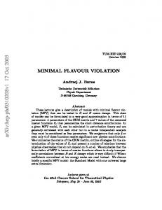
Figure 1: The overview of the determination of various quantities discussed in the text with results given in Table 2. Explicitly for central values of parameters we find (using (13)) q v(ηcc , ηct ) p 1 + h(ηcc , ηct )S(v) − 1, v(ηcc , ηct ) = 0.0282, |Vcb| = p ξS(v)

h(ηcc , ηct ) = 24.83 .

(29) The second solution of the quadratic equation for |Vcb|2 is excluded as it leads to a negative |Vcb|2 . The numerical values of h(ηcc , ηct ) and v(ηcc , ηct ) correspond to the central values of ηcc and ηct in Table 1. We will discuss the uncertainty due to these parameters in the next section. With all this information at hand we can determine |Vub |, |Vts | and |Vtd | as functions of S(v). q ˆB FB from (8) and knowing already Step 3: Finally having |Vcb | we can determine B d d q ˆBs FBs . ξ from Step 1 also B

As the route to determine all these quantities could appear not transparent we show it in a chart in Fig. 1.

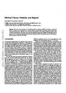
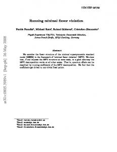
In Fig. 2 we show the dependence of ξ on γ varying SψKS in its one σ range. We note that the uncertainty due to SψKS is very small. This triple correlation is universal for all CMFV models including the SM and is central for tests of CMFV framework. Measuring γ from tree-level decays precisely together with precise values of SψKS and ξ will be an important test for this class of models as this correlation is independent of S(v). The range for γ in (27) has been extracted from this plot by varying ξ and SψKS independently in their present one σ ranges.

3 Numerical Analysis

9 80 75

Γ @° D

70 65 60 55 50 1.15

1.20

1.25

1.30

Ξ

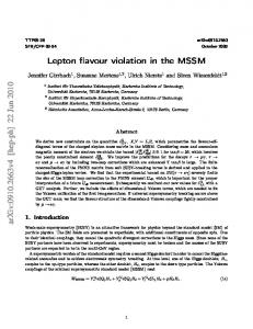
Figure 2: γ versus ξ for SψKS ∈ [0.659, 0.699]. It should be emphasized that this first test is independent of |Vub | and |Vcb| and can become a precision test of CMFV models. But in order to find out which CMFV model, if any, is chosen by nature we have to consider the quantities which depend on S(v). This brings us to Steps 2 and 3. The S(v) and γ dependence of all quantities of interest is shown in Table 2. We show there also the SM case corresponding to S(v) = S0 (xt ) = 2.31. These results are also shown in Fig. 3, where we plot various quantities as functions of S(v) for different values of γ. The thickness of the lines shows the uncertainty in SψKS . Evidently these plots are correlated with each other: • Once one of the variables is determined, also S(v) is determined and consequently the remaining quantities are predicted. • In a given model in which S(v) is known, all quantities considered are predicted. Equivalently to Fig. 3 one can find using (20) explicit universal correlations between various quantities in Table 2. We show few examples below. In all plots we also show the present best values of all quantities obtained directly from lattice or tree-level decays. In order to understand the results let us recall the problems of CMFV for q in Table 2q ˆBs and FB B ˆB in Table 1 [10, 11]. With the value the present input for |Vcb |, FBs B d d of β extracted from SψKS and γ from ∆Ms /∆Md , εK is in the SM significantly smaller than its experimental value, while ∆Ms,d are significantly larger than corresponding experimental values. Therefore increasing S(v), while bringing εK closer to the data, shifts ∆Ms,d further from their experimental values. Using for example |Vub | = 0.0034 and γ = 68◦ where the SM prediction and the central experimental value for SψKS coincide, the SM prediction for |εK |SM = 0.00186 is below the data. Turning now to CMFV, the value of S(v) at which the central experimental value of |εK | is reproduced turns out to be S(v) = 2.9 [11] to be compared with SSM = 2.31. At this value of S(v) with present input the central values of ∆Ms,d read ∆Md = 0.69(6) ps−1 ,

∆Ms = 23.9(2.1) ps−1 .

(30)

3 Numerical Analysis

S(v)

γ

2.31

63◦

10

|Vcb|

|Vub|

|Vtd |

|Vts |

FBs

q

ˆBs B

FBd

q

ˆB B d

ξ

B(B + → τ + ν)

43.6

3.69

8.79

42.8

252.7

210.0

1.204

0.822

2.5

63

◦

42.8

3.63

8.64

42.1

247.1

205.3

1.204

0.794

2.7

63◦

42.1

3.56

8.49

41.4

241.8

200.9

1.204

0.768

2.31

67◦

42.9

3.62

8.90

42.1

256.8

207.2

1.240

0.791

67

◦

42.2

3.56

8.75

41.4

251.1

202.6

1.240

0.765

2.7

67

◦

41.5

3.50

8.61

40.7

245.7

198.3

1.240

0.739

2.31

71◦

42.3

3.57

9.02

41.5

260.8

204.5

1.276

0.770

2.5

71◦

41.6

3.51

8.87

40.8

255.1

200.0

1.276

0.744

2.7

◦

40.9

3.45

8.72

40.1

249.6

195.7

1.276

0.719

2.5

71

Table 2: CMFV predictions for various quantities as functions of S(v)qand γ. The four q ˆBs and FB B ˆB in units of elements of the CKM matrix are in units of 10−3 , FBs B d d MeV and B(B + → τ + ν) in units of 10−4 . They both differ from experimental values by 3σ. Using another value of |Vub | which worsen the agreement of the SM with the experimental value for SψKS leads to a different value of S(v) to reproduce |εK |exp = 0.002228 and thus also (30) changes.

These problems of CMFV can also be seen when the present central values of |Vcb| and of non-perturbative parameters are inserted together with the data on ∆Ms,d , εK , |Vcb| and |Vus | into (20). We find then SψKS = sin 2β = 0.86 ⇒ β = 29.8◦ ,

Rt = 0.92

(31)

and thus Rb = 0.50 ,

|Vub | = 0.0047 ,

γ = 66.4◦ .

(32)

Evidently, the fact that SψKS is much larger than the data requires the presence of new CP-violating phases. This exercise is equivalent to the one performed in [5], where εK has been set to its experimental value but sin 2β was predicted. On the other hand setting SψKS to its experimental value as done in [6] one finds that |εK | is significantly below the data. q q ˆ ˆB Thus the only hope for CMFV is that the input on |Vcb |, FBs BBs and FBd B d changes with time. In particular as seen in Table 2: q q ˆ ˆB have to decrease significantly, at least as • The values of FBs BBs and FBd B d far as given in (26). But this assumes the lowest value of S(v).

3 Numerical Analysis

11

5.0

ÈVub È @10-3 D

ÈVcb È @10-3 D

43

42

41

4.5 4.0 3.5

40

3.0

2.3

2.4

2.5

2.6

2.7

2.8

2.3

2.4

2.5

5.0

5.0

4.5

4.5

4.0 3.5

2.8

2.6

2.7

2.8

2.6

2.7

2.8

4.0 3.5

3.0 2.3

2.7

SHvL

ÈVub È @10-3 D

ÈVub È @10-3 D

SHvL

2.6

3.0 2.4

2.5

2.6

2.7

2.8

2.3

2.4

2.5

SHvL

SHvL

9.0 42.5 ÈVts È @10-3 D

ÈVtd È @10-3 D

8.9 8.8 8.7 8.6

41.5 41.0 40.5

8.5 2.3

42.0

40.0 2.4

2.5

2.6

2.7

2.8

2.3

SHvL

2.4

2.5 SHvL

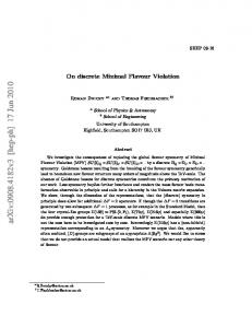
Figure 3: CKM matrix elements versus S(v) for γ = 63◦ /67◦ /71◦ (green, red, blue). The thickness of the lines corresponds to the 1σ range of SψKS ∈ [0.659, 0.699]. • At this value of S(v) in order to obtain agreement of εK with the data |Vcb | should be larger by roughly 2σ from its present central tree-level value. • Increasing S(v) allows q to lower theqrequired value of |Vcb | but simultaneously ˆBs and FB B ˆB making their values significantly lower decreases further FBs B d

d

than their present values without changing their ratio (see Fig. 4). This finding shows that the freedom in choosing S(v) does not necessarily help in solving CMFV problems.

• With increasing γ the value of q |Vcb | required by εK can further be decreased. For q ˆBs but decreases FB B ˆB as can be read off a fixed S(v) this increases FBs B d d

12

44

44

43

43 ÈVcb È @10-3 D

ÈVcb È @10-3 D

4 The Uncertainty due to ηcc and ηct

42 41 40 39 190

42 41 40

200

210 220 ` 12 FBd B Bd @MeVD

230

240

39 230

240

250

260 270 280 ` 12 FBs B Bs @MeVD

290

300

q q ˆ ˆBs for S(v) ∈ [2.3, 2.8] and γ ∈ [63◦ , 71◦ ] Figure 4: |Vcb | versus FBd BBd and FBs B ◦ ◦ (yellow), γ = 63◦ /67◦/71◦ (green, q = 2.4 and γ ∈ [63 , 71 ]. q red, blue). Cyan: fixed S(v) ˆB = 226(13) MeV, FBs B ˆBs = 279(13) MeV and Gray range: 1σ range of FB B d

d

|Vcb| = (40.9 ± 1.1) × 10−3 (see Table 1). from Fig. 4.

• For the full range of S(v) and γ considered in Table 2 the values of |Vub | and |Vtd | remain in the following ranges: |Vub| = (3.57 ± 0.16) × 10−3,

|Vtd | = (8.75 ± 0.26) × 10−3

(33)

where in the case of |Vub| we included also the error from β, which is irrelevant in the case of |Vtd |. Otherwise the error in |Vub | would amount to ±0.12. The value of |Vts | follows the one of |Vcb | but is by 1.9% smaller than the latter. Also for B(B + → τ + ν) a narrow range is predicted: B(B + → τ + ν) = (0.77 ± 0.07) × 10−4 ,

(34)

where the present uncertainty in FB+ has been taken into account. q ˆB and |Vcb| In Fig. 4 on the left hand side we show the correlation between FBd B d q ˆBs and |Vcb | is shown on for different value of γ. Analogous correlation between FBs B the right hand side. Possibly these two plots showing the allowed ranges for the three parameters in question in the CMFV framework are the most important result of our paper. Similarly we show in Fig. 5 the same correlation but with |Vub|.

4

The Uncertainty due to ηcc and ηct

It is known that significant uncertainty in the SM prediction for εK comes from the value of the QCD correction ηcc and to a lesser extent from ηct that even at the NNLO

4 The Uncertainty due to ηcc and ηct

13

4.6 4.4

4.5 ÈVub È @10-3 D

ÈVub È @10-3 D

4.2 4.0 3.8 3.6 3.4

4.0

3.5

3.2 3.0 190

3.0 200

210 220 ` 12 FBd B Bd @MeVD

230

240

230

240

250

260 270 280 ` 12 FBs B Bs @MeVD

290

300

q q ˆB and FBs B ˆBs for S(v) ∈ [2.3, 2.8] and γ ∈ [63◦ , 71◦ ] Figure 5: |Vub| versus FBd B d ◦ ◦ (yellow), γ = 63◦ /67◦/71◦ (green, q = 2.4 and γ ∈ [63 , 71 ]. q red, blue). Cyan: fixed S(v) ˆB = 226(13) MeV, FBs B ˆBs = 279(13) MeV and Gray range: 1σ range of FB B d

excl |Vub |

= (3.21 ± 0.31) × 10 Table 1).

ηct

h(ηcc , ηct ) 0.451 0.496 0.541

−3

d

(light gray), |Vubincl | = (4.41 ± 0.31) × 10−3 (dark gray) (see

ηcc 1.10 1.87 2.64 18.83 34.93 85.82 15.57 24.83 51.42 11.61 18.55 34.21

ηct

v(ηcc , ηct ) 0.451 0.496 0.541

ηcc 1.10 1.87 2.64 0.0303 0.0259 0.0207 0.0323 0.0282 0.0235 0.0341 0.0304 0.0260

Table 3: Coefficient h(ηcc , ηct ) and v(ηcc , ηct ) in Eq. (29) for different values of ηcc,ct. level are known only with the accuracy of ±41% and ±9%, respectively [47, 48]. In our analysis this uncertainty enters the coefficient h(ηcc , ηct ) of S(v) and v(ηcc , ηct ) in (29). In what follows we would like to investigate the impact of these uncertainties on the determination of |Vcb| from εK and propose a method how the uncertainty in ηcc could be reduced with the help of the experimental value of ∆MK accompanied in particular by future lattice calculations of long distance effects in ∆MK . In Table 3 we show the values of h(ηcc , ηct ) corresponding to the range of these QCD corrections calculated in [47, 48]. If we fix γ = 67◦ and S(v) = S0 (xt ) = 2.31 and vary ηcc ∈ [1.10, 2.64] and ηct ∈ [0.451, 0.541] simultaneously then |Vcb | lies within the range [41.7, 44.4] · 10−3 (see also Fig. 6). Scanning only ηcc (ηct ) and fixing ηct (ηcc ) to its central value we find |Vcb | ∈ [42.1, 43.9] · 10−3(|Vcb | ∈ [42.6, 43.4] · 10−3 ). Translated in the uncertainty in the determination of |Vcb| we find an uncertainty of ±2.0% and ±0.9% due to ηcc and ηct , respectively. The uncertainty due to ηtt is fully negligible. It is expected that an improved matching of short distance calculations of ηcc and ηct ˆK can significantly reduce the present total theoretical to the lattice calculations of B error on εK and thus allow a more accurate extraction of |Vcb |.

4 The Uncertainty due to ηcc and ηct

14 ÈVcb È @103 D

0.54

0.52

Η3

44 43.5

0.50

43 42.5 42

0.48

0.46 1.5

2.0

2.5

Η1

Figure 6: |Vcb| as a function of ηcc and ηct for fixed γ = 67◦ and S(v) = S0 (xt ) = 2.31. As the large uncertainty in ηcc is disturbing we propose to extract this parameter from the experimental value of ∆MK . Assuming that in CMFV models ∆MK is fully dominated by the SM contributions we decompose it as follows: ∆MK = (∆MK )cc + (∆MK )ct + (∆MK )tt + (∆MK )LD ,

(35)

with the first three short distance contributions obtained from K (∆MK )ij = 2ℜ(M12 )ij

(36)

K with M12 given in (17) and i = c, t. For the dominant contribution we have

(∆MK )cc = (λ −

λ3 2 G2F 2 ˆ ) F BK mK ηcc m2c (mc ) . 2 6π 2 K

We find then setting mc (mc ) at its central value4   0.75 w, ηcc = 2.123 ˆK B

(37)

(38)

where (k = tt, ct, LD) w = 1 − rtt − rct − rLD , 4

rk =

(∆MK )k . (∆MK )exp

(39)

In principle the determination of ηcc xc is more useful as this product should be independent of the scale µc in mc but in order to compare with the value of ηcc in Table 1 we prefer here to work with ηcc .

4 The Uncertainty due to ηcc and ηct

15

For rtt and rct we find within the SM rtt = 0.0021,

rct = 0.0030

(40)

confirming the result in [47] that both corrections are below 1% and totally negligible within the SM compared with other uncertainties. As our analysis shows in CMFV models rtt could be increased by 30% due to the increase of S(v) but this would still keep these corrections below 1%. Thus our proposal depends crucially on the estimate of rLD . Yet, as we argue below the error from this contribution is significantly smaller than the error from the direct NNLO calculation in [47]. Basically the only results on rLD in QCD that are available are from large N QCD calculations in which at low energies one uses a dual representation of QCD as a theory ¯ 0 mixing and non-leptonic of weakly interacting mesons [51–53]. In the case of K 0 − K K-meson decays this approach, developed in [22, 23, 54–56], provided already a quarter of century ago results which are now basically confirmed by the more sophisticated ˆK parameter calculated first in [22, 23] lattice calculations. This is the case of the B and also the case of ∆I = 1/2 rule [56], where the dynamics behind this rule related predominantly to current-current operators has been identified and the enhancements of ∆I = 1/2 transitions and suppression of ∆I = 3/2 transitions have been computed reaching rough agreement with the data. Precisely this understanding is presently emerging from lattice calculations [57, 58]. Motivated by the success of this approach, its results for rLD could also be approximately correct.. The leading in N contribution comes from one-loop contributions induced by two ∆S = 1 transitions with virtual ππ, πK and KK in the loop. One finds then rLD to be positive and in the ballpark of 0.3 [59, 60]. The study of subleading corrections ˆK these corrections are not large and tend to indicates that similarly to the case of B cancel partly each other [22, 34, 61, 62] with some tendency to have opposite sign to the leading term [62]. While precise calculation of rLD in view of these cancellations is very difficult by analytic methods, based on these studies we expect that rLD is likely to be positive and in the ballpark of 0.1 − 0.3. Taking this estimate at face value and using (38) we end up with ηcc ≈ 1.70 ± 0.21. (41)

This is consistent with ηcc = 1.87 used by us in the previous section. Moreover, the error is by a factor of 3-4 smaller than the error obtained by the direct NNLO calculation of ηcc in [47]. Interestingly the authors of the latter paper would find this result if they varied the scale µc in the range 1.3 ≤ µc ≤ 1.8 GeV and not in the range 1.0 − 2.0 GeV.

Needless to say, we are aware of the fact that these expectations and the estimate in (41) require more detailed investigations and in particular future confirmation from lattice simulations. Presently no reliable result on rLD from lattice is available but an important progress towards its evaluation has been made in [63]. This first result seems to indicate that rLD could be larger than expected by us. We are therefore looking forward to more precise evaluation of this important quantity from the lattice in order to see whether also in this case large N approach passed another test or not.

16

45

45

44

44

43

43

ÈVcb È @10-3 D

ÈVcb È @10-3 D

5 Going Beyond CMFV

42 41 40 39

42 41 40

190

200

210 220 ` 12 FBd B Bd @MeVD

230

240

39 230

240

250

260 270 280 ` 12 FBs B Bs @MeVD

290

300

q ˆ ˆBs for γ ∈ [63◦ , 71◦ ]. The yellow region Figure 7: |Vcb| versus FBd BBd and FBs B is the same as in Fig. 4: S(v) ∈ [2.31, 2.8], ηcc = 1.87, ηct = 0.496. In the purple region we include the errors in ηcc,ct as in Table 3: S(v) ∈ [2.31, 2.8], ηcc ∈ [1.10, 2.64], ηct ∈ [0.451, 0.541]. In the cyan region we use instead the reduced error of ηcc as in Eq. (41): S(v) ∈ [2.31, 2.8], ηcc ∈ [1.49, 1.91], ηct ∈ [0.451, 0.541]. In the blue region we fix ηct to its central value: S(v) ∈ [2.31, 2.8], ηcc ∈ [1.49, 1.91], ηct = 0.496. To test the SM we include the black region for fixed S(v) = S0 (xt ) = 2.31 and ηcc,ct as in the purple region. The gray line within the black SM region corresponds to ηcc = 1.87 and ηct = 0.496. The gray box is the same as in Fig. 4. q

In Fig. 7 we show the anatomy of various uncertainties with different ranges described in the figure caption. We observe that the reduced error on ηcc corresponding to the cyan region decreased the allowed region which with future lattice calculations could be decreased further. Comparing the blue and cyan regions we note that the reduction in the error on ηct would be welcomed as well. It should also be stressed that in a given CMFV model with fixed S(v) the uncertainties are reduced further. This is illustrated with the black range for the case of the SM. Finally an impact on Fig. 7 will have a precise measurement of γ or equivalently precise lattice determination of ξ. We illustrate this impact in Fig. 8 by setting in the plots of Fig. 7 γ = (67 ± 1)◦ .

5

Going Beyond CMFV

It is evident from our analysis and inq particular fromqFig. 4 that in the likely case in ˆBs and FB B ˆB will only change by a few which the central values of |Vcb|, FBs B d d percent but their uncertainties will be significantly reduced, one will have to look beyond the CMFV framework to understand the ∆F = 2 data. Models like Littlest Higgs model with T-parity, various Randall-Sundrum scenarios and general supersymmetric models having many free parameters will be able to remove all these tensions although improved precision on the quantities in question would imply new constraints on the parameters of these models. Here we mention simpler models were the discussion can be made

17

45

45

44

44

43

43

ÈVcb È @10-3 D

ÈVcb È @10-3 D

5 Going Beyond CMFV

42 41 40 39

42 41 40

190

200

210 220 ` 12 FBd B Bd @MeVD

Figure 8: |Vcb| versus FBd

q

230

240

ˆB and FBs B d

q

39 230

240

250

260 270 280 ` 12 FBs B Bs @MeVD

290

300

ˆBs as in Fig. 7 but for γ = (67 ± 1)◦ . B

more transparent than in those more complicated models. First in the case of MFV at large [64–66] in which new operators can contribute the situation looks a bit better. Here the presence of left-right scalar operators in a 2HDM or the MSSM naturally interferes destructively with the SM contribution suppressing in particular ∆Ms [67], but only slightly ∆Md and having no impact on εK . Even if in these models charged Higgs and SUSY particles can enhance S(v) one can expect that still values q of |Vcb| willqbe required to be above the ones quoted in Table 1 and the ones ˆBs and FB B ˆB have to be suppressed. But the problem will be softer than of FBs B d

d

in CMFV. On the other hand left-right operators affect the ratio ∆Ms /∆Md which in CMFV models agrees well with data. The solution then would be left-left scalar operators which affect ∆Ms and ∆Md by the same factor and keep this ratio fixed.

The latter solution appears to be the best for the 2HDM with flavour blind phases, the so-called 2HDMMFV [68, 69] as well. But here the presence of new CP-violating phases changes the situation radically as now |Vub| can be chosen larger in order to fit εK . The enhanced value of sin 2β can be suppressed through these new phases. This implies on the other hand enhancement of the asymmetry Sψφ to values 0.15 − 0.20 [11] which is 2σ above the central experimental value from LHCb and could be ruled out when the data improve. Possibly the simplest solution to the problems of various models with MFV is to reduce the flavour symmetry U(3)3 to U(2)3 [70–76]. As pointed out in [26] in this case NP 0 ¯ 0 are not correlated with each other so that the enhancement effects in εK and Bs,d −B s,d of εK and suppression of ∆M q q s,d can be achieved if necessary in principle for the values ˆBs and FB B ˆB in Table 1. of |Vcb|, FBs B d

d

In particular,

• NP effects in εK are of CMFV type and εK can only be enhanced but the size of necessary enhancement depends on the value of |Vub | which similar to 2HDMMFV does not have to be low.

6 Conclusions

18

0 ¯ 0 system, the ratio ∆Ms /∆Md is equal to the one in the SM and in • In Bs,d −B s,d good agreement with the data. But in view of new CP-violating phases ϕBd and ϕBs even in the presence of only SM operators, ∆Ms,d can be suppressed. But the U(2)3 symmetry implies ϕBd = ϕBs and consequently a triple SψKS − Sψφ − |Vub | correlation which constitutes and important test of this NP scenario [26].

• The important advantage of U(2)3 models over 2HDMMFV is that in the case of Sψφ being very small or even having opposite sign to SM prediction, this framework can survive with concrete prediction for |Vub |.

6

Conclusions

q q ˆBs , FB B ˆB , |Vcb|, |Vub |, |Vtd | and |Vts |, In this paper we have determined FBs B d d necessary to fit very precise data on εK , ∆Md , ∆Ms and SψKS in CMFV models as functions of the phase γ and the sole NP free parameter in the ∆F = 2 transitions, the value of the box diagram function S(v). An important ingredient of this analysis was a ˆK from lattice and the fact that B ˆK comes within 1 − 2% from its very small error on B large N value 0.75. The results are shown in Table 2 and Figs. 3-5. The chart showing the execution of our strategy can be found in Fig. 1. Our main messages from this analysis are as follows: • The tension between εK and ∆Ms,d in CMFV models accompanied with |εK | being smaller than the data within the SM, cannot be removed by varying S(v) when the present input parameters in Table 1 are used. q ˆBs and • Rather the value of |Vcb | has to be increased and the values of FBs B q ˆB decreased relatively to the presently quoted lattice values. These enFBd B d hancements and suppressions are correlated with each other and depend on γ. The allowed regions in the space of these three parameters, the most important results of our paper, are shown in Figs. 4, 7 and 8. • The knowledge of long distance contributions to ∆MK accompanied by the very precise experimental value of the latter allows a significant reduction of the present uncertainty in the value of the QCD factor ηcc under the plausible assumption that ∆MK in CMFV models is fully dominated by the SM contribution. This implies the reduction of the theoretical error in εK and in turn the reduction of the error in the extraction of the favoured value of |Vcb | in the CMFV framework. Present estimates of these long distance contributions using large N QCD allow for an optimism but more sophisticated lattice calculations are required to fully execute this idea.

REFERENCES

19

We have also discussed simplest extensions of the SM which could in principle offer a better description of the data in case CMFV would fail to do so. Models with U(2)3 flavour symmetry appear to us as most efficient in this respect while being still very simple. In order to see whether the CMFV framework will survive final tests from ∆F = 2 transitions further progress from lattice calculations and experimental measurements is required. Our wish list includes: q q ˆ ˆB and ξ but also • In particular improved lattice calculations of FBs BBs , FBd B d ˆ ˆ ˆ of BK , BBs and BBs . • Calculation of long distance contribution to ∆MK in order to reduce the error on ηcc as proposed by us. • Improved experimental data on |Vcb |, |Vub|, γ, SψKS and Sψφ . In particular a measurement of Sψφ significantly different from 0.04 would signal the presence of new phases beyond the CMFV framework. The correlations identified in this paper will allow to monitor the future developments, likely to indicate that new sources of flavour and CP-violation beyond the CMFV framework are present in nature. In this context our main message is the following one. While until now the search for NP through rare decays did not bring any convincing signs of its presence, it could turn out soon that ∆F = 2 transitions combined with the progress made by lattice community will herald the appearance of particular type of NP. This would not only be exciting news but would also give some directions for searching for this NP in rare decays and even high-energy processes. Acknowledgements We thank Jean-Marc G´erard for many illuminating comments and Chris Sachrajda for useful information on the progress in lattice calculations. This research was fully financed and done in the context of the ERC Advanced Grant project “FLAVOUR” (267104).

References [1] A. J. Buras, P. Gambino, M. Gorbahn, S. Jager, and L. Silvestrini, Universal unitarity triangle and physics beyond the standard model, Phys. Lett. B500 (2001) 161–167, [hep-ph/0007085]. [2] A. J. Buras, Minimal flavor violation, Acta Phys. Polon. B34 (2003) 5615–5668, [hep-ph/0310208]. [3] M. Blanke, A. J. Buras, D. Guadagnoli, and C. Tarantino, Minimal Flavour Violation Waiting for Precise Measurements of ∆Ms , Sψφ , AsSL , |Vub |, γ and 0 → µ+ µ− , JHEP 10 (2006) 003, [hep-ph/0604057]. Bs,d

REFERENCES

20

[4] M. Blanke and A. J. Buras, Lower bounds on ∆Ms,d from constrained minimal flavour violation, JHEP 0705 (2007) 061, [hep-ph/0610037]. [5] E. Lunghi and A. Soni, Possible Indications of New Physics in Bd -mixing and in sin(2β) Determinations, Phys. Lett. B666 (2008) 162–165, [arXiv:0803.4340]. [6] A. J. Buras and D. Guadagnoli, Correlations among new CP violating effects in ∆F = 2 observables, Phys. Rev. D78 (2008) 033005, [arXiv:0805.3887]. [7] UTfit Collaboration Collaboration, M. Bona et. al., An Improved Standard Model Prediction Of BR(B → τ ν) And Its Implications For New Physics, Phys.Lett. B687 (2010) 61–69, [arXiv:0908.3470]. [8] A. Lenz, U. Nierste, J. Charles, S. Descotes-Genon, A. Jantsch, et. al., Anatomy ¯ mixing, Phys.Rev. D83 (2011) 036004, of New Physics in B − B [arXiv:1008.1593]. [9] E. Lunghi and A. Soni, Possible evidence for the breakdown of the CKM-paradigm of CP-violation, Phys.Lett. B697 (2011) 323–328, [arXiv:1010.6069]. [10] A. J. Buras, M. V. Carlucci, L. Merlo, and E. Stamou, Phenomenology of a Gauged SU(3)3 Flavour Model, arXiv:1112.4477. [11] A. J. Buras and J. Girrbach, BSM models facing the recent LHCb data: A First look, Acta Phys.Polon. B43 (2012) 1427, [arXiv:1204.5064]. [12] C. Davies, Standard Model Heavy Flavor physics on the Lattice, PoS LATTICE2011 (2011) 019, [arXiv:1203.3862]. [13] E. G´amiz, Flavour physics from lattice QCD, arXiv:1303.3971. [14] Y. Aoki, R. Arthur, T. Blum, P. Boyle, D. Brommel, et. al., Continuum Limit of BK from 2+1 Flavor Domain Wall QCD, Phys.Rev. D84 (2011) 014503, [arXiv:1012.4178]. [15] T. Bae, Y.-C. Jang, C. Jung, H.-J. Kim, J. Kim, et. al., BK using HYP-smeared staggered fermions in Nf = 2 + 1 unquenched QCD, Phys.Rev. D82 (2010) 114509, [arXiv:1008.5179]. [16] ETM Collaboration Collaboration, M. Constantinou et. al., BK -parameter from Nf = 2 twisted mass lattice QCD, Phys.Rev. D83 (2011) 014505, [arXiv:1009.5606]. [17] G. Colangelo, S. Durr, A. Juttner, L. Lellouch, H. Leutwyler, et. al., Review of lattice results concerning low energy particle physics, Eur.Phys.J. C71 (2011) 1695, [arXiv:1011.4408].

REFERENCES

21

[18] J. A. Bailey, T. Bae, Y.-C. Jang, H. Jeong, C. Jung, et. al., Beyond the Standard ¯ 0 mixing, PoS LATTICE2012 (2012) 107, Model corrections to K 0 − K [arXiv:1211.1101]. [19] S. Durr, Z. Fodor, C. Hoelbling, S. Katz, S. Krieg, et. al., Precision computation of the kaon bag parameter, Phys.Lett. B705 (2011) 477–481, [arXiv:1106.3230]. [20] J. Laiho, E. Lunghi, and R. S. Van de Water, Lattice QCD inputs to the CKM unitarity triangle analysis, Phys. Rev. D81 (2010) 034503, [arXiv:0910.2928]. Updates available on http://latticeaverages.org/. [21] B. D. Gaiser, T. Tsao, and M. B. Wise, Parameters of the six quark model, Annals Phys. 132 (1981) 66. [22] A. J. Buras and J.-M. G´erard, 1/N Expansion for Kaons, Nucl.Phys. B264 (1986) 371. [23] W. A. Bardeen, A. J. Buras, and J.-M. G´erard, The B Parameter Beyond the Leading Order of 1/N Expansion, Phys.Lett. B211 (1988) 343. [24] J.-M. G´erard, An upper bound on the Kaon B-parameter and Re(ǫK ), JHEP 1102 (2011) 075, [arXiv:1012.2026]. [25] UTfit Collaboration Collaboration, M. Bona et. al., Model-independent constraints on ∆ F=2 operators and the scale of new physics, JHEP 0803 (2008) 049, [arXiv:0707.0636]. Updates available on http://www.utfit.org. [26] A. J. Buras and J. Girrbach, On the Correlations between Flavour Observables in Minimal U(2)3 Models, JHEP 1301 (2013) 007, [arXiv:1206.3878]. [27] A. J. Buras, F. De Fazio, J. Girrbach, and M. V. Carlucci, The Anatomy of Quark Flavour Observables in 331 Models in the Flavour Precision Era, JHEP 1302 (2013) 023, [arXiv:1211.1237]. [28] A. J. Buras, F. De Fazio, and J. Girrbach, The Anatomy of Z’ and Z with Flavour Changing Neutral Currents in the Flavour Precision Era, JHEP 1302 (2013) 116, [arXiv:1211.1896]. [29] A. J. Buras, J. Girrbach, and R. Ziegler, Particle-Antiparticle Mixing, CP Violation and Rare K and B Decays in a Minimal Theory of Fermion Masses, arXiv:1301.5498. [30] A. J. Buras, R. Fleischer, J. Girrbach, and R. Knegjens, Probing New Physics with the Bs → µ+ µ− Time-Dependent Rate, arXiv:1303.3820. [31] A. J. Buras, F. De Fazio, J. Girrbach, R. Knegjens, and M. Nagai, The Anatomy of Neutral Scalars with FCNCs in the Flavour Precision Era, arXiv:1303.3723.

REFERENCES

22

[32] S. H. Kettell, L. Landsberg, and H. H. Nguyen, Alternative technique for standard model estimation of the rare kaon decay branchings BR(K → πν ν¯) (SM), Phys.Atom.Nucl. 67 (2004) 1398–1407, [hep-ph/0212321]. [33] A. J. Buras, F. Parodi, and A. Stocchi, The CKM matrix and the unitarity triangle: Another look, JHEP 0301 (2003) 029, [hep-ph/0207101]. [34] A. J. Buras, D. Guadagnoli, and G. Isidori, On ǫK beyond lowest order in the Operator Product Expansion, Phys.Lett. B688 (2010) 309–313, [arXiv:1002.3612]. [35] M. Blanke, A. J. Buras, K. Gemmler, and T. Heidsieck, ∆F = 2 observables and B → Xq γ in the Left-Right Asymmetric Model: Higgs particles striking back, JHEP 1203 (2012) 024, [arXiv:1111.5014]. [36] R. Dowdall, C. Davies, R. Horgan, C. Monahan, and J. Shigemitsu, B-meson decay constants from improved lattice NRQCD and physical u, d, s and c sea quarks, arXiv:1302.2644. [37] Particle Data Group Collaboration, K. Nakamura et. al., Review of particle physics, J.Phys.G G37 (2010) 075021. [38] Particle Data Group Collaboration, J. Beringer et. al., Review of Particle Physics (RPP), Phys.Rev. D86 (2012) 010001. [39] K. Chetyrkin, J. Kuhn, A. Maier, P. Maierhofer, P. Marquard, et. al., Charm and Bottom Quark Masses: An Update, Phys.Rev. D80 (2009) 074010, [arXiv:0907.2110]. [40] HPQCD Collaboration Collaboration, I. Allison et. al., High-Precision Charm-Quark Mass from Current-Current Correlators in Lattice and Continuum QCD, Phys.Rev. D78 (2008) 054513, [arXiv:0805.2999]. [41] A. J. Buras, M. Jamin, and P. H. Weisz, Leading and next-to-leading QCD ¯ 0 mixing in the presence of a heavy top corrections to ε parameter and B 0 − B quark, Nucl. Phys. B347 (1990) 491–536. [42] J. Urban, F. Krauss, U. Jentschura, and G. Soff, Next-to-leading order QCD ¯ 0 mixing with an extended Higgs sector, Nucl. Phys. corrections for the B 0 − B B523 (1998) 40–58, [hep-ph/9710245]. [43] CDF Collaboration, D0 Collaboration Collaboration, T. Aaltonen et. al., Combination of the top-quark mass measurements from the Tevatron collider, Phys.Rev. D86 (2012) 092003, [arXiv:1207.1069]. [44] Heavy Flavor Averaging Group Collaboration, Y. Amhis et. al., Averages of B-Hadron, C-Hadron, and tau-lepton properties as of early 2012, arXiv:1207.1158.

REFERENCES

23

[45] LHCb collaboration Collaboration, R. Aaij et. al., Measurement of CP violation and the Bs0 meson decay width difference with Bs0 → J/ψK + K − and Bs0 → J/ψπ + π − decays, arXiv:1304.2600. [46] LHCb Collaboration Collaboration, G. Raven, Measurement of the CP violation phase φs in the Bs system at LHCb, arXiv:1212.4140. [47] J. Brod and M. Gorbahn, Next-to-Next-to-Leading-Order Charm-Quark Contribution to the CP Violation Parameter εK and ∆MK , Phys.Rev.Lett. 108 (2012) 121801, [arXiv:1108.2036]. [48] J. Brod and M. Gorbahn, ǫK at Next-to-Next-to-Leading Order: The Charm-Top-Quark Contribution, Phys.Rev. D82 (2010) 094026, [arXiv:1007.0684]. [49] C. Tarantino, Flavor Lattice QCD in the Precision Era, arXiv:1210.0474. [50] R. Fleischer and R. Knegjens, In Pursuit of New Physics with Bs0 → K + K − , Eur.Phys.J. C71 (2011) 1532, [arXiv:1011.1096]. [51] G. ’t Hooft, A Planar Diagram Theory for Strong Interactions, Nucl.Phys. B72 (1974) 461. [52] G. ’t Hooft, A Two-Dimensional Model for Mesons, Nucl.Phys. B75 (1974) 461. [53] E. Witten, Baryons in the 1/n Expansion, Nucl.Phys. B160 (1979) 57. [54] W. A. Bardeen, A. J. Buras, and J.-M. G´erard, The ∆I = 1/2 Rule in the Large N Limit, Phys.Lett. B180 (1986) 133. [55] W. A. Bardeen, A. J. Buras, and J.-M. G´erard, The K → ππ Decays in the Large N Limit: Quark Evolution, Nucl.Phys. B293 (1987) 787. [56] W. A. Bardeen, A. J. Buras, and J.-M. G´erard, A Consistent Analysis of the ∆I = 1/2 Rule for K Decays, Phys.Lett. B192 (1987) 138. [57] T. Blum, P. Boyle, N. Christ, N. Garron, E. Goode, et. al., Lattice determination of the K → (ππ)I=2 Decay Amplitude A2 , arXiv:1206.5142. [58] RBC Collaboration, UKQCD Collaboration Collaboration, P. Boyle et. al., Emerging understanding of the ∆I = 1/2 Rule from Lattice QCD, arXiv:1212.1474. [59] J. Bijnens, J.-M. G´erard, and G. Klein, The KL − KS mass difference, Phys.Lett. B257 (1991) 191–195. [60] J.-M. G´erard, Electroweak interactions of hadrons, Acta Phys.Polon. B21 (1990) 257–305.

REFERENCES

24

[61] J. F. Donoghue, E. Golowich, and B. R. Holstein, Long Distance chiral contributions to KL − KS mass difference, Phys.Lett. B135 (1984) 481. [62] J.-M. G´erard, C. Smith, and S. Trine, Radiative kaon decays and the penguin contribution to the ∆I = 1/2 rule, Nucl.Phys. B730 (2005) 1–36, [hep-ph/0508189]. [63] N. Christ, T. Izubuchi, C. Sachrajda, A. Soni, and J. Yu, Long distance contribution to the KL − KS mass difference, arXiv:1212.5931. [64] R. S. Chivukula and H. Georgi, Composite technicolor standard model, Phys. Lett. B188 (1987) 99. [65] L. J. Hall and L. Randall, Weak scale effective supersymmetry, Phys. Rev. Lett. 65 (1990) 2939–2942. [66] G. D’Ambrosio, G. F. Giudice, G. Isidori, and A. Strumia, Minimal flavour violation: An effective field theory approach, Nucl. Phys. B645 (2002) 155–187, [hep-ph/0207036]. [67] A. J. Buras, P. H. Chankowski, J. Rosiek, and L. Slawianowska, Correlation between δms and b0d,s → µ+ µ− in supersymmetry at large tan β, Phys. Lett. B546 (2002) 96–107, [hep-ph/0207241]. [68] A. J. Buras, M. V. Carlucci, S. Gori, and G. Isidori, Higgs-mediated FCNCs: Natural Flavour Conservation vs. Minimal Flavour Violation, JHEP 1010 (2010) 009, [arXiv:1005.5310]. [69] A. J. Buras, G. Isidori, and P. Paradisi, EDMs versus CPV in Bs,d mixing in two Higgs doublet models with MFV, Phys.Lett. B694 (2011) 402–409, [arXiv:1007.5291]. [70] R. Barbieri, G. Isidori, J. Jones-Perez, P. Lodone, and D. M. Straub, U(2) and Minimal Flavour Violation in Supersymmetry, Eur.Phys.J. C71 (2011) 1725, [arXiv:1105.2296]. [71] R. Barbieri, P. Campli, G. Isidori, F. Sala, and D. M. Straub, B-decay CP-asymmetries in SUSY with a U(2)3 flavour symmetry, Eur.Phys.J. C71 (2011) 1812, [arXiv:1108.5125]. [72] R. Barbieri, D. Buttazzo, F. Sala, and D. M. Straub, Flavour physics from an approximate U(2)3 symmetry, JHEP 1207 (2012) 181, [arXiv:1203.4218]. [73] R. Barbieri, D. Buttazzo, F. Sala, and D. M. Straub, Less Minimal Flavour Violation, JHEP 1210 (2012) 040, [arXiv:1206.1327]. [74] A. Crivellin, L. Hofer, and U. Nierste, The MSSM with a Softly Broken U(2)3 Flavor Symmetry, PoS EPS-HEP2011 (2011) 145, [arXiv:1111.0246].

REFERENCES

25

[75] A. Crivellin, L. Hofer, U. Nierste, and D. Scherer, Phenomenological consequences of radiative flavor violation in the MSSM, Phys.Rev. D84 (2011) 035030, [arXiv:1105.2818]. [76] A. Crivellin and U. Nierste, Supersymmetric renormalisation of the CKM matrix and new constraints on the squark mass matrices, Phys.Rev. D79 (2009) 035018, [arXiv:0810.1613].