Strong solutions to a class of boundary value problems on a mixed ...

arXiv:1501.05901v1 [math.AP] 23 Jan 2015

Strong solutions to a class of boundary value problems on a mixed Riemannian–Lorentzian metric Antonella Marini1 and Thomas H. Otway2 1

Dipartimento di Matematica, Universit`a di L’Aquila, 67100 L’Aquila, Italy 1,2 Department of Mathematical Sciences, Yeshiva University, New York, New York 10033 Abstract A first-order elliptic-hyperbolic system in extended projective space is shown to possess strong solutions to a natural class of Guderley–Morawetz– Keldysh problems on a typical domain. Key words: Elliptic–hyperbolic equations, extended projective disc, symmetric positive operators. MSC2010 Primary: 35M32; Secondary: 35Q75, 58J32

1

Introduction

Although there is a large literature on elliptic–hyperbolic boundary value problems associated with the transition from subsonic to supersonic flow, the literature on boundary value problems that arise from the transition between a Riemannian and a Lorentzian metric is proportionally rather sparse. For reviews, see [12] and [16]; see also [1]. In this note we prove the existence of strong solutions to an elliptic–hyperbolic boundary value problem for a lowerorder perturbation of the Laplace–Beltrami equation on the extended projective disc P2 . In this problem the underlying Beltrami metric [2, 17] undergoes a transition from Riemannian to Lorentzian signature along the absolute, the curve at infinity, which is the unit circle in R2 . See, e.g., Sec. 9.1 of [4] for discussion. The equations considered here are motivated by at least two topics in spacetime geometry. First, the Laplace–Beltrami equation on extended P2 is the hodograph image of the equation for extremal surfaces in Minkowski space M3 . That equation has the form # " ∇u = 0, ∇· p |1 − |∇u|2 | 1

where the unknown function u (x, y) denotes the graph of the surface. See Sec. 6.1 of [13], and the references cited therein, for discussion. Second, harmonic fields on extended P2 have an interpretation as a toy model for waves on certain relativistically rotating cylinders. A rotating, axisymmetric cylindrical solution to the Einstein equations has the general form
ds2 = −A(r)dt2 + 2B(r)dφdt + C(r)dφ2 + D(r) dr2 + dz 2 , where t, z ∈ R; r ∈ R+ ; and φ ∈ [0, 2π] . This metric has Lorentzian character provided the quantity AC + B 2 exceeds zero. Consider the special case of a cylinder rotating at angular velocity ω and satisfying

ds2 = −dt2 + 2ωr2 dφdt + r2 1 − ω 2 r2 dφ2 + F (r) dr2 + dz 2 , (1.1) where  r 0 and |γ1 | ≥ 4 |Γ1 (1 − y 2 )| These conditions are necessary and sufficient for the matrix Q in eq. (2.8) to be positive on Ω. Conditions (2.3) can be satisfied provided Γ is bounded, and the domain is bounded in the x-direction, and bounded away from the lines y 2 = 1 in the y-direction. If we take f2 ≡ 0, then eq. (2.2) is transformed into a condition for complete integrability; see the discussions in Sec. 6 of [9] and Secs. 3

1–3 of [8]. If f2 is assumed to be nonvanishing, then (2.2) becomes a condition for helicity in the sense of [14], Sec. 5.4. We assume that f1 is not identically zero, so that we can impose trivial boundary data without obtaining a trivial solution; by linearity an inhomogeneous system with homogeneous boundary data can be shown to be equivalent to a homogeneous differential equation having inhomogeneous boundary data; see Sec. 2.6 of [13]. Write eqs. (2.1, 2.2) as the matrix equation       1 − x2 −xy u1 −xy 1 − y 2 u1 + + 0 −1 u2 x 1 0 u2 y      −2x + γ1 −2y u1 f1 = . (2.4) −Γ2 Γ1 u2 f2 The system (2.4) is not symmetric as a matrix equation, so we solve for u2x in (2.2) to obtain u2x = u1y − u1 Γ2 + u2 Γ1 . Substituting this equation into eq. (2.1) yields

1 − x2 u1x − xy (2u1y − u1 Γ2 + u2 Γ1 ) + 1 − y 2 u2y − (2x − γ1 ) u1 − 2yu2 = f1 , or

1 − x2 u1x − 2xyu1y + 1 − y 2 u2y + (xyΓ2 + γ1 − 2x) u1 − (xyΓ1 + 2y) u2 = f1 .

(2.5)

Also, we write in place of (2.2),

1 − y 2 (u1y − u2x − u1 Γ2 + u2 Γ1 ) = 1 − y 2 f2 .

(2.6)

Equation (2.6) is equivalent to (2.2) for our choice of Ω. We obtain the matrix operator L defined by       1 − x2 0 u1 −2xy 1 − y 2 u1 LU = + + 0 y2 − 1 1 − y2 0 u2 x u2 y    xyΓ2 + γ1 −
2x −xyΓ1 − 2y u1
≡ A1 Ux + A2 Uy + BU. (2.7) u2 Γ2 y 2 − 1 Γ1 1 − y 2 Writing B∗ =

B+B 2

T

 =

xyΓ2 + γ1 − 2x −xyΓ1 −2y+Γ2 (y 2 −1) 2

we obtain B∗ −

−xyΓ1 −2y+Γ2 (y 2 −1) 2
Γ1 1 − y 2


1 1 Ax + A2y ≡ Q, 2 4

 ,

(2.8)

where Q11 = xyΓ2 + γ1 , Q12 = Q21 =


−xyΓ1 Γ2 2 + y −1 , 2 2

and
Q22 = Γ1 1 − y 2 . In order for the operator L to be symmetric positive on Ω in the sense of [3], we require that Q11 be positive, which will be satisfied by condition (2.3), and that the matrix determinant
2
1 xyΓ1 + y 2 − 1 Γ2 |Q| = γ1 Γ1 1 − y 2 − 4 also be positive. The latter condition will also follow from (2.3) provided y 2 is bounded above away from 1 on Ω; this is insured in the following section.

3

Admissibility of the boundary conditions

Define nj , j = 1, 2 to be the components of the outward-pointing normal. Adopting the summation convention for repeated indices, we write

  1 − x2 n1 − 2xyn2 1 − y 2
n2
β = nj Aj = . 1 − y 2 n2 y 2 − 1 n1 Writing [11]  

2 n1 2 n2 + 2xy − 1 − x n2 , α= − 1−y n1 n2 wherever this object exists we can write β in the alternate form !

n2 1 − y 2
n2 −α − 1 −
y 2 n12 β= . 1 − y 2 n2 y 2 − 1 n1

(3.1)

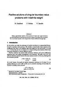
We will consider boundary value problems in the context of the following geometry. Let Ω include the unit disc D1 in R2 centered at the origin of coordinates, truncated at the north and south “polar caps” by the curves n  1/2 o C = (x, y) |y = ± 1 − x2 − h (x) , (3.2) where h is a function chosen so that 0 ≤ h(x) ≤ 1 − x2 and the graph of C is C 2 on ∂Ω. The boundary of Ω is completed in the second and third quadrants by the polar lines√L1 and√L2 , which are tangent to the unit circle at (for example)
the points − 2/2, ± 2/2 . Let h vanish at those points. Polar lines have an independent interest in the geometry of extended P2 ; c.f. Figure 6.3 of [13]. See Figure 1, which illustrates Ω for particular choices of h, L1 , and L2 . Note that the geometry of the domain is rather typical for boundary value problems 5

Figure 1: Geometry of a typical domain. Hatched lines indicate curves which are not boundary arcs. An arbitrarily small smoothing curve at the corner has been omitted for clarity associated with equations of Keldysh type; c.f. Figures 3.2, 3.4, 4.8, and 6.4–6.6 of [13]. Make the canonical choice n1 = dy and n2 = −dx, under a “right-handed” orientation (with the domain interior on the left when the boundary is traversed in the counter-clockwise direction). We find that αdy = 0 is the equation of characteristic lines to eqs. (2.5, 2.6) and ∀ (x, y) ∈ D1 ,

αdy = − 1 − y 2 dx2 − 2xydxdy − 1 − x2 dy 2 ≤ 2

−x2 dx2 − 2xydxdy − y 2 dy 2 = − (xdx + ydy) ≤ 0.

(3.3)

Equation (3.3) implies that on any arc τ1 , contained in D1 , on which dy > 0, we have α ≤ 0. On τ1 write β = β+ + β− with   −α 0 β+ = 0 0 and β− = 1 − y

2




 n2

− nn21 1

1 − nn12

 .

Choose the boundary condition β− U = 0, that is, − u1 n2 + u2 n1 = u1 dx + u2 dy = 0. With this choice of β+ and β− we have ∗

β+ − β− = µ = µ =


n2 −α + 1 −
y 2 n12 y 2 − 1 n2 6

!
y 2 − 1
n2 . 1 − y 2 n1

(3.4)


Then µ∗11 ≥ 0 and |µ∗ | = −α 1 − y 2 n1 ≥ 0 for n1 = dy ≥ 0. Equation (3.3) implies that on any arc τ2 , contained in D1 , on which dy < 0, we have α ≥ 0. On τ2 write β = β+ + β− with   −α 0 β− = 0 0 and adopt the boundary condition β− U = 0, that is, u1 = 0. Choose
β+ = 1 − y 2 n 2



− nn12 1

(3.5) 1 − nn12



so that ∗

β+ − β− = µ = µ =


n2 α + y 2 −
1 n21 1 − y 2 n2

!
1 − y 2
n2 . y 2 − 1 n1

Then µ∗11 ≥ 0 and on any arc within the closure of the unit disc,
|µ∗ | = αn1 y 2 − 1 ≥ 0.

(3.6)

On the characteristic lines, α = 0. Then choosing β± as on arc τ2 , β− becomes the zero matrix; so no boundary conditions need to be imposed on the characteristic lines. In this case !

n2 2 2 2 1 − y n y − 1
n1
2 . µ∗ = 1 − y 2 n2 y 2 − 1 n1 Then µ∗11 ≥ 0 as, by construction, n1 = dy is non-positive on the characteristic arcs of ∂Ω, and |µ∗ | = 0. A boundary value problem in which boundary conditions are imposed everywhere except on the characteristic lines is called a Guderley–Morawetz problem. In our problem there is an additional unconventional feature: the ellipticity of the system degenerates on part of the elliptic boundary. Such problems have been studied by Keldysh [5], and for that reason we refer to the boundary value problem introduced in this section as a Guderley–Morawetz–Keldysh problem. However, in distinction to the problem studied in [5], in this case the elliptic degeneracy plays no role in the analysis. This is an illustration of the powerful type-independence of Friedrichs’ method.

3.1

Singularities and corners

The matrix β in the alternate form (3.1) has an apparent singularity at points for which n1 = 0. The geometry of the boundary implies that n1 will change sign at no less than two points of ∂Ω – and more than two for some choices of h. 7

However, this apparent singularity in (3.1) is removable by simply writing out the terms of α and noticing that the singular terms in (3.1) cancel additively (for all values of n1 ). There is a corner at the intersection of the polar lines (Figure 1). Note that the equations do not change type at this corner, and that the rank of the matrix β does not change there. However the conditions of [15] for regularity at a corner are not satisfied; for example, |µ∗ | vanishes at the corner. (See however, [6], an approach which we do not use.) Interpolate an arbitrarily small smoothing curve at the corner. Then n1 = dy < 0 at this corner; n2 = −dx is non-negative for y ≥ 0 and non-positive for y ≤ 0. Choose

  1 − x2 n1 − 2xyn2 1 − y 2
n2 β+ = 0 y 2 − 1 n1 and β− = β − β+ . The change of sign in n2 on the x-axis is benign, conditions (3.5) are satisfied by β− U, and µ∗ ≥ 0. So the boundary conditions assigned previously to the set τ2 can be applied to an arbitrarily small smoothing curve at the corner, and such curves are naturally a subset of τ2 . For all our choices of β± , the intersection of the ranges of β+ and β− contains only the zero vector. Moreover, the null spaces of β± span the restriction to the boundary of the solution space for the system. These properties are required for admissibility in the sense of [3]. In their absence, the boundary conditions are only semi-admissible, and only the existence of a weak solution follows from the methods of [3].

4

Result

The arguments of Section 2 and 3 imply that the methods of [3], which have become standard, can be applied to complete the proof of the following theorem: Theorem 4.1. Let Ω ⊂ R2 be the union of the unit disc D1 , flattened slightly near the poles by the curves C given by (3.2), and the subset of the complement of D1 which is bounded by the polar lines L1 and L2 . These lines initiate at the points (x0 , y0 ) in the second and third quadrants at which h (x0 ) = 0 and terminate at an intersection point (x1 , 0) , where x1 < −1. (The corner at this intersection can be smoothed to C 2 without violating the hypotheses or conclusions of this theorem.) Assume that the prescribed 1-forms Γ1 and Γ2 do not have blow-up singularities on Ω and that condition (2.3) is satisfied. Then the system (2.1, 2.2), with γ2 ≡ 0 and (f1 , f2 ) ∈ L2 (Ω), supplemented by the boundary condition (3.4) on the set τ1 ∈ Ω\G, the boundary condition (3.5) on the set τ2 ∈ Ω\G, and no boundary conditions at all on the set G = L1 ∪ L2 , possesses a strong solution in Ω.

8

References [1] J. Barros-Neto and F. Cardoso, Gellerstedt and Laplace–Beltrami operators relative to a mixed signature metric, Ann. Mat. Pura Appl. 188 (2009), 497–515. [2] E. Beltrami, Saggio di interpretazione della geometria non-euclidea, Giornale di Matematiche 6 (1868), 284–312. [3] K. O. Friedrichs, Symmetric positive linear differential equations, Commun. Pure Appl. Math. 11 (1958), 333–418. [4] J. Heidmann, Relativistic Cosmology, An Introduction. Springer-Verlag, Berlin-Heidelberg-New York (1980). [5] M. V. Keldysh, On certain classes of elliptic equations with singularity on the boundary of the domain [in Russian], Dokl. Akad. Nauk SSSR 77 (1951), 181–183. [6] P. D. Lax and R. S. Phillips, Local boundary conditions for dissipative symmetric linear differential operators, Commun. Pure Appl. Math. 13 (1960), 427–455. [7] F. Lobo and P. Crawford, Time, closed timelike curves, and causality, in: The Nature of Time: Geometry, Physics and Perception (NATO ARW), Proceedings of a conference held 21-24 May, 2002 at Tatranska Lomnica, Slovak Republic. Edited by Rosolino Buccheri, Metod Saniga, and William Mark Stuckey. NATO Science Series II: Mathematics, Physics and Chemistry - Volume 95. Dordrecht/Boston/London: Kluwer Academic Publishers, 2003. [8] A. Marini and T. H. Otway, Nonlinear Hodge–Frobenius equations and the Hodge–B¨ acklund transformation, Proc. R. Soc. Edinburgh 140A (2010), 787–819. [9] T. H. Otway, Nonlinear Hodge maps. J. Math. Phys. 41 (2000), 5745–5766. [10] T. H. Otway, Hodge equations with change of type. Ann. Mat. Pura Appl. 181 (2002), 437–452. [11] T. H. Otway, Harmonic fields on the projective disk and a problem in optics, J. Math. Phys. 46 (2005), 113501. (Erratum: J. Math. Phys. 48 (2007), 079901.) [12] T. H. Otway, Variational equations on mixed Riemannian-Lorentzian metrics. J. Geom. Phys. 58 (2008), 1043–1061. [13] T. H. Otway, The Dirichlet Problem for Elliptic-Hyperbolic Equations of Keldysh Type, Lecture Notes in Mathematics, Vol. 2043, Springer-Verlag, Berlin-Heidelberg-New York-Tokyo, 2012. 9

[14] T. H. Otway, Elliptic–Hyperbolic Partial Differential Equations: a minicourse in geometric and quasilinear methods, Springer-Verlag, in press. [15] L. Sarason, On weak and strong solutions of boundary value problems, Commun. Pure Appl. Math. 15 (1962), 237–288. [16] J. M. Stewart, Signature change, mixed problems and numerical relativity. Class. Quantum Grav. 18 (2001), 4983–4995. [17] J. Stillwell, Sources of Hyperbolic Geometry. Amer. Math. Soc., Providence, 1996. [18] W. J. van Stockum, The gravitational field of a distribution of particles rotating about an axis of symmetry, Proc. R. Soc. Edinburgh 57 (1937), 135–154. [19] F. J. Tipler, Rotating cylinders and the possibility of global causality violation, Phys. Rev. D9 (1974), 2203–2206. [20] C. G. Torre, The helically reduced wave equation as a symmetric positive system, J. Math. Phys. 44 (2003), 6223-6232.

10