Structure and Parameter Identification for a Two-Mass-System with ...

STRUCTURE- AND PARAMETER IDENTIFICATION FOR A TWO-MASS SYSTEM WITH BACKLASH AND FRICTION USING A SELF-ORGANIZING MAP F. Schütte, S.Beineke , H. Grotstollen, N. Fröhleke, U. Witkowski, U. Rückert, S. Rüping

University of Paderborn, Germany

Abstract. A self-commissioning system for high performance speed and position control of electrical drives requires a structure and parameter identification of a nonlinear mechanic as basic building block. This self-commissioning system in combination with a new identification scheme is presented here. The identification is based on extraction of characteristic features from the system response and evaluation of these features by self-organizing neural networks, especially the Self-Organizing feature Map (SOM).

Keywords. Self-commissioning, identification, nonlinear two-mass system, self-organizing neural network

1 INTRODUCTION

MFCM, µFM

controlled system

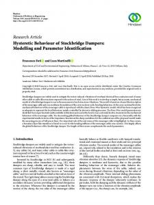
The speed and position control loops include the dynamics of the mechanical transfer elements and of the working machine to be controlled, both of which show some kind of mechanical imperfections, such as elasticity, backlash and friction. For high dynamic speed control of electrical drives these mechanical imperfections have to be considered, which implies the need for an identification of these mechanical parameters during commissioning. But so far, application of advanced methods for examination of structure and parameters as well as the determination of an appropriate controller for a given mechanic can only be performed by highly qualified personnel and can be very time consuming. Industrial application of advanced control methods becomes only feasible when system identification and controller adjustment will be carried out almost automatically. The key of success in a self-commissioning scheme for speed and position control of electrical drives is a system identification that works also well in the presence of nonlinearities like backlash and friction. In many practical applications it is sufficient for control design to model the physical multi-body system as a two-mass system. This model, shown in Fig. 1, is characterized by the following parameters which have to be identified: Motor side inertia J M , load side inertia J L , stiffness C F and damping constant D F of the elastic coupling, total width of backlash 2s and parameters for Coulomb ( M FC ) or viscous ( µ F ) friction. In this paper the damping constant and the friction of the motor side are assumed to be very small. In contrast to the parameters of the mechanic, the time constant of the current control loop T Ei and the torque constant K M are usually known. Besides these physical parameters the values • total inertia J Σ = J M + J L , • ratio of load side inertia to motor side inertia V J = J L ⁄ J M , • natural frequency ω o = C F J Σ ⁄ ( J M J L ) , • relative damping d = ω o D F ⁄ ( 2C F ) • and eigenfrequency ω e = 2πf e = ω o 1 − d 2 , which is for small damping nearly the same as the natural frequency, can be used as more normalized values to describe the system. Most of the identification schemes for two-mass systems presented in the past are based on determination of continuous or discrete time transfer functions and are thus limited to linear problems, like determination of eigenfrequency, damping and inertias [3], [4], [5]. Usually the identification methods applied to two-mass systems assume very small backlash values and neglect nonlinear friction effects. In some cases Coulomb friction is considered by adding appropriate parameters to the linear difference equation of the model, see e.g. [6]. Another way to cope with nonlinear friction effects is to drive the system at constant speed and to consider the friction torque as a constant external load torque. This approach implies an already working speed controller and estimation methods that can cope with correlated input/output signals,

mechanical part (two-mass-system)

electrical part

KM

Generation of torque signal

TEi+Tt

MM*

MM

MFM

closed loop current control

1 ωΜ

CF

MW

Measurement Recording

JM

1

εΜ

s DF

ωΜ

1

JL

ML

Figure 1: Signal flow chart of two mass system

∆ε

−s

MM

MFL

1 ωL

εL

MFCL, µFL

that are inevitable when operating in closed speed control loop. In contrast to conventional approaches in this article a new method for nonlinear system identification [8] is presented which can be characterized by the following steps: • Excitation of the mechanical system by a torque signal which is adapted automatically to the properties of the plant • Recording the system response using only information about motor speed and current • Extraction of characteristic features from system response and evaluation of patterns with a Self-Organizing Map (SOM) [1] to identify the system By sequential evaluation of different SOMs during the identification process it is possible, in contrast to strictly model based methods, to distinguish between different structures before performing the identification of parameters. The different structures are given by dominant characteristics of the mechanic, which depend of course on the parameters, especially on the product ω e T Ei and on a normalized backlash value s N = sC F 1; e.g. it is valid to approximate a very stiff system without backlash as one-mass system or to neglect small backlash for systems with low stiffness, but not for systems with high stiffness. This leads in comparison to Fig. 1 to reduced model structures, e.g. an onemass system or a two-mass system without backlash. Taking this into account, it is obvious that the different structures are represented by characteristic features of the system responses, which can be at first extracted and afterwards evaluated with parameter specific SOMs during the course of identification. Thus, a step-by-step identification procedure results. 1. The ratio sC F ⁄ M Lmin ,where M Lmin is the minimal load torque, see [2], is a suitable measure for the influence of backlash on a cloosed loop control.

Because the identification scheme is integrated in a self-commissioning system, this system is briefed before outlining structure and parameter identification. Afterwards the validity of the proposed identification method is checked investigating mechanics with more than 1000 different parameter combinations in simulative studies. To demonstrate advantages and disadvantages of the method, the results are compared to those obtained by an iterative application of an instrumental variables method (IV4) [4]. 2 SELF-COMMISSIONING SYSTEM The self-commissioning system as depicted in Fig. 2 is proposed. It comprises of three levels for commissioning. The lowest level, called „Control“ is formed by the plant, which consists of the mechanical system to be controlled and the torque controlled drive, the sensor equipment and speed or position controllers. operator Man-MachineInterface à priori knowledge of total system

control specifications

Knowledge Base

fault diagnostics control and adaptation algorithms

test signals

method [3] is implemented. Using the proposed controller parameters as initial values, in most cases a quick, and, regarding stability, uncritical opimization is possible. The three levels of the self-commissioning system indicate how information is represented. The two lowest levels work mainly on the base of measurement data, while the transition to the knowledge base lead to an extraction of essential information from data. This information is presented in symbolic form, which is expressed by the symbol-dataconversion blocks in Fig. 2. During identification process the system is excited at the lowest level and the measurement data is recorded. The identification algorithm, located at the second level, transforms the data into physical parameters, which is a kind of symbolic information. These parameters can e.g. be visualized for the operator, a task which is performed by the knowledge base, located at the highest level. Because the knowledge base can deal with high level (symbolic) information, experience from commissioning engineers can be imported in form of fuzzy-rules or by using a graphical interface. Because of the symbol-data-conversion the commissioning is reduced to essential aspects, which leads to an immense simplification. Furthermore it is envisaged to use the results of the off-line and on-line identification for monitoring the state of the drive system, hence conduct fault diagnostics. 3 STRUCTURE AND PARAMETER IDENTIFICATION 3.1 Course of Identification

off-line identification algorithms

on-line identification algorithms

SELECTION

parameters

SELECTION

structure

S/D

S/D

First a suitable excitation is selected, applied to the system and its response is recorded, which is outlined in 3.2. The idea of STEP 2 is to split the model of the two-mass system in its one-mass system approximation plus an additive term, which describes the oscillation. For systems without viscous friction and without backlash the validity of STEP 2 can be proven analytically, because the transfer function can be written as

S/D

Identification structure and parameter identification "learning model"

Control (adaptive) controller

plant

Figure 2: Self-commissioning system

The general course of identification, which is integrated in the selfcommissioning system, can be taken from Table 1. Except some inputs from the commissioning engineer STEP 1 to 4 are carried out automatically.

sensor equipment

S/D : Symbol-Data-Conversion

On the second level, called „Identification“, the system´s structure and parameters are identified. In a more advanced version of the self-commissioning drive control also on-line identification in combination with adaptive control will be feasible, which is outlined in [10],[11]. The highest level of this hierarchical system, called „Knowledge Base“, controls the course of the self-commissioning process and serves for communication with an operator, e.g. a commissioning engineer. Its function during self-commissioning can be described as follows: The knowledge base selects test signals automatically, which are applied to the system to be controlled, yielding responses for the identification of the system´s structure and parameters. For the off-line identification process appropriate algorithms are chosen to extract characteristic features. The analysis is carried out by SOMs. Identification results are validated by the knowledge base and after this check structure and parameters are indicated to the operator. The results of identification together with control specifications fixed by the commissioning engineer - e.g. decision wether speed or position control is demanded, requirements of dynamic or stationary accuracy, etc. - are evaluated by the knowledge base, which automatically infers a proposal for the controller concept and its parameters. Therefore suitable control concepts have been selected (e. g. [2], [9]). They are investigated concerning performance and operation ranges regarding relevant control specifications. As a result rules are derived, which are stored in the knowledge base. Optional an automatic on-line fine-tuning of the controller parameters is possible after the down-load of the proposed controller concept. Therefore a suitable optimization algorithm using a Simplex search

ωM ( s) =

M M ( s ) − M FC sgn ( ω L ) sJ Σ JL

s JΣ

  , M ( s ) + M FC ( s )  JM M  s2 + 2dω + ω 2 o o ω M ( s ) = ω M ( s ) + ω osc ( s ) . +

(1)

Extensive simulations are showing the validity of this approach also for systems containing backlash and viscous friction. Approximating the systems response in the different sections I to VI (see Table 1 STEP 1) yields the signal ω M ( t ) . The total inertia and the coefficients of Coulomb and viscous friction are derived in the same step. For this task many identification methods have been found to be suitable, because the signal/noise ratio for determination of these parameters is usually high; e.g. a simple least squares algorithm [4] can be applied. In STEP 3 structure identification based on the oscillating part of the system response, ω osc ( t ) = ω M ( t ) − ω M ( t ) , is carried out to decide about the best model structure for the unknown mechanic. A specific SOM, see Fig. 7, is well suited for structure identification and it is used, in conjunction with the shape of the signal ω osc ( t ) , to classify the following structures, see also Table 1: • Stiff systems without backlash: (Nearly) no oscillation in the speed signal; sometimes this classification may be wrong for systems with a low ratio V J , because of weak feedback to the motor side, caused by a very small shaft torque. • Elastic systems without backlash: The oscillation is dominated by the elasticity, nevertheless there can be a negligible backlash. • Elastic systems with backlash: The oscillation is affected by elasticity and backlash; not only one characteristic is dominant.

• Stiff systems with backlash: The oscillation is dominantly characterized by the effects of backlash, the stiffness is high.

I

II

ωM [rad/s]

20

III

IV

V

7.5

VI

5.0

ω Mmax

10

2.5

0

0

-10

-2.5

-20

0.7M*

0

-5.0

M*

-30 0.5

1

1.5

STEP 2: System approximation as one-mass system

• commonly used identification methods

10 ωM

ωM

5

0 0

0.05

0.1

0.15

0.2 t [s]

2

ωM-ωM [rad/s]

STEP 3: Structure recognition Extraction of oscillation • Projection • Filtering Extraction of features • FFT (frequency domain) • features in time domain Analysis of features • SOM

2

15

ωM,ωM [rad/s]

Identification of J Σ , M FC , µ F

-7.5 t [s]

1

-1

0.05

0.1

0.15

0.2 t [s]

STEP 4: Identification of specific two-mass system parameters stiff systems without backlash

elastic systems without backlash

already identified

Identification of f e , V J , ( d ) • SOM • other identification methods, e.g IV4, LS

Regarding these demands, various test signals were analysed resulting in a strategy for a step-by-step adaptation of the test signal to the specific plant. This strategy operates without having much a-priori knowledge about the system under test. The motor torque is altered stepwise, depending on a limit of the motor speed ± ω Mmax , between five discrete values ( ± 0.7M* , ± M* , 0 ) (see Table 1 STEP 1), so that speed and position on the one hand are constrained to limited ranges and on the other hand they are zero at the end of the test period. This is realized by a switching speed controller and leads to an output signal, that can be divided into six different sections, indicated by roman numbers I...VI. Starting with some small values a suitable excitation of the system is found after a few iterations. Either the values M* and ω Mmax are selected automatically by the knowledge base, in which some rules for adaptation of M* and ω Mmax are stored, or they can be changed by the commissioning engineer. In comparison to additive test signals applied to the mechanic operating in a closed speed control loop with linear controller, the used measure has the advantage, that the input signal is nearly uncorrelated with the output.

0

-2 0

To acquire data the mechanical system is excited by an appropriate test signal, using the torque controlled motor as actuator. A common applicable test signal should have the following features: • simple and automatic generation • sufficient excitation of the system without causing any damage to machines • applicability for a wide range of different plants

elastic systems with backlash

stiff systems with backlash

Identification of f e , V J , ( d ) , s • SOM Identification of backlash s in speed controlled system pattern recognition in motor torque signal [7] (sinusoidal reference )

Table 1: Course of automatic identification (The methods outlined in this paper are printed in bold characters.) For stiff systems without backlash it is assumed, that the mechanic can be sufficiently modelled by the parameters already identified in STEP 1. For elastic systems without backlash and stiff or elastic systems with backlash different characteristics (see 3.3) were found to extract information about the physical parameters in STEP 4. As long as the system behaves almost linear, as elastic systems without backlash do, well known standard identification methods work sufficiently, e.g. those based on transfer function in time or frequency domain. In the presence of backlash the SOM method proposed in this paper is applied, because it is more robust for systems with increasing nonlinearity. If the system belongs to a structure with backlash, the identification of backlash can be performed after determination of the parameters f e , J Σ and V J by the method described in [7]. To utilize this method the parameters of the linear model have to be known to drive the system well in speed controlled mode with a sinusoidal reference. The backlash is estimated by extracting features from the motor torque, which contains information about the backlash at that times, when the load side discouples from the motor side and when the load couples in again after going through the backlash. Based on our experiences it is recommended to use a similar step by step course also for identification schemes, which base on determination of transfer functions. Of course, these methods will not work satisfactory for systems containing not negligible backlash. For a more comparative study one may refer to [12].

3.3 Characteristic features Fig. 3 depicts the systems responses of two systems with different parameters. The left response corresponds to an elastic system with an eigenfrequency of 20 Hz and without backlash. In contrast the right response belongs to a more stiff system with an eigenfrequency of 80 Hz and backlash of 0.4 ° . Differences in the behaviour of both systems are obvious, both in the time domain and in the frequency domain. The idea is now to extract these obvious differences as characteristic features and to find a correlation between these features and the system´s structure and parameters. Intuitively or by some physical insight characteristic features can be derived, which are dominantly correlated with a single mechanical parameter. Such parameter specific features can be evaluated by SOMs, which leads to "parameter specific maps". These maps contain a relation between physical parameters and features, as described in 3.4. The search for suitable features is an iterative procedure of extracting features and their analysis. In the following some characteristic features are presented that were b)

a) ωM / [rad/s]

30

Selection of excitation and data acquisition

ΜΜ [Nm]

STEP 1:

3.2 Excitation of the system

30

30

25

25

20

20

15

15

10 I

5 0 0.8

10

II

I

II

5 0.9

1

t / [s]

0 0.8

1.1

0.9

1

1.1 t / [s]

10

10 II

II

vj,i vj,i 5

0

5

1

10

2

f / [Hz]

10

0

1

10

2

f / [Hz]

10

Figure 3: Features in time and frequency domain ( v j, i indicates one element of a feature vector, see 3.4) a) Speed signal and FFT of a system without backlash b) Speed signal and FFT of a system dominated by backlash

Characteristic features for identification of eigenfrequency To extract the dominant frequency of the system, features in the frequency domain are extracted. They are calculated as follows: Basis of extraction is the oscillation signal ω osc ( t ) of the system response, as shown in STEP 3 of Table 1. The system´s response ω osc ( t ) of each section (see STEP 1) is transformed into the frequency domain by performing a fast Fourier transformation (FFT), which is normalized to the range [ 0, 10 ] . For linear elastic systems the eigenfrequency is given by the dominant frequency f d of the FFT, e.g. f d = f e = 20Hz in Fig. 3(a). To detect also the eigenfrequency for systems containing backlash, e.g. f e = 80Hz, f d = 47Hz in Fig. 3(b), more advanced preprocessing becomes necessary. Due to the varying number of samples in the frequency domain depending on the length of the time signal the frequency samples are reduced to a fixed number of 25 by summing and weighting neighboured samples. The ratio of window width of summarized frequency samples and middle frequency of a window is constant, which ensures an equal window width when plotted in logarithmic scale. This results in the bars plotted in the lower part of Fig. 3. Calculating mean values over all six signal sections, the heigth of the resulting bars are forming the feature vector. Additionally the feature vector is completed by the index position of the highest spectral amplitude. Altogether the feature vector for detecting the dominant frequency consists of 26 components. Characteristic features for structure recognition Another feature vector is used for structure recognition, where the normalized backlash value s N was found as suitable measure for the influence of backlash. Here features in the frequency domain are used, too. Because the value of dominant frequency is insignificant in this context, a normalized time signal is basis of calculation, derived from the oscillating term ω osc of each section. After estimation of the dominant frequency in the time signal it is downsampled to yield a minimum of 10 samples per oscillation period. The first two periods of the resulting signal are transformed into the frequency domain, where the main peak is always at f d , as shown in Fig. 4. b) 1 a) 1 II

the cylindrical object in Fig. 6. The objective of the map is to learn the structure of the n-dimensional input space and to reflect it on the twodimensional map. Normally n is larger than the map dimension. A great advantage of this neural network type is the ability of unsupervised learning, because there is no need to classify the learning data by hand in advance. For instance, different system parameters may result in the same system behavior, which is recognized by the map. The map learns from the input data only and is self-organizing. This is different to a multilayer perceptron (supervised learning) for instance, where in the learning phase the input and the output vector is needed. After learning the obtained knowledge is represented by these maps and can be used for identification. Generally the process needed for identification can be divided into two phases, called „Training of the map, Learning“ and „Recall of the map, Identification“, indicated in Fig. 5 and outlined in the following. SOM training

"Learning" (Knowledge aquisition) two-mass system feature extraction

test signals plant

"Identifiction"

recall from SOM

0.8

0.6

0.6

Training of the map, Learning: Reference data is generated by extensive simulation of two-mass systems with different parameters. Afterwards characteristic features are extracted from the system responses. For classification of different simulated models the feature vectors v j are extracted as outlined in 3.3 and then used for training the map. feature v  1  vector  v2     v  n j

x

vj,i 0.4

= weight vector

y

0.4 vj,i

0.2 0 0

= best match

0.2

1

2

3 f/fd

4

5

0 0

structure, parameters

Figure 5: Flow diagram of system identification

II

0.8

parameter specific SOMs

…

used to train the SOM for structure recognition, see STEP 3, and the SOM for identification of eigenfrequency, see STEP 4.

1

2

3 f/fd

4

5

Figure 4: Components of feature vector (section II) for C F s map a) System without backlash b) System dominated by backlash Fig. 4a has been calculated from the system response of the purely elastic system. There is only one significant amplitude at f ⁄ f d = 1 , but in contrast Fig. 4(b) shows additional spectral lines at double and tripple dominat frequency due to the triangle like oscillation caused by backlash. The spectrum is normalized to the signal energy to calculate the feature vector, which leads to an amplitude of nearly one at the dominant frequency caused by harmonic oscillation and a decreasing value when the signal contains higher harmonics. The feature vector is composed of 8 samples in frequency domain indicated by the small circles in Fig. 4 using amplitudes at dominant and higher frequencies. 3.4 Use of Self-Organizing Maps for identification Because SOMs are used for identification some of their special features are summarized below: In order to analyse patterns extracted from system responses SOMs are used which were developed by Kohonen [1]. The SOM is a special neural network, composed of a two-dimensional rectangular array of neurons, forming a competition layer. A single neuron is represented by a n-dimensional vector, called the weight vector w j , symbolized by

Figure 6: Two dimensional Self-Organizing Map with input vector v j Training of the map starts with a random initialization of the weights; every weight vector component of each neuron is set up randomly by a number between zero and the maximum range. Then the n-dimensional feature vectors v j are combined to a learning record of m vectors. For training the SOM the euclidean distances between an input vector and all weight vectors have to be calculated. The neuron having the minimum distance to the input vector is called best match, emphasized by the dark gray in Fig. 6. The best match position (index bm) related to vector v j is calculated by v j − w bm

= min ( v j − w i ) . i

(2)

After determing the best match neuron the weight vectors w i of the best match and the surrounding neurons are adapted to the input vector to make them more similar according to wi ( k + 1) = wi ( k) + h ( k) [ vj ( k) − wi ( k) ] ,

(3)

with the neighbourhood function h ( k ) and the learning step k . h ( k ) depends on the learning step k and the distance between the best match position and the neuron to be adapted. The longer the distance the smaller is the adaptation strength, i.e. the best match neuron is shifted mostly to the input vector. The lighter gray in the neighbourhood of the best match, see Fig. 6, symbolizes a decreasing value of h ( k ) . At the

a) f e [Hz]

beginning of the learning process h ( k ) reaches a wide area around the best match, which decreases during the training. Due to this training method the n-dimensional input space will be transformed to the twodimensional map preserving its topology. Neighboured vectors of the input space will be represented near each other on the map. For identification this means, that similar systems will activate the same neurons or clusters of neurons at recall.

150 100 50

All SOMs, which have been used for identification, have a size of 40 by 40 neurons. Every parameter specific map has been trained ten times by a record of 1800 feature vectors, which have been calculated as described in 3.3, from 1800 system responses with different parameter combinations. A smooth surface in Fig. 7 and Fig. 8, which are respective representations for parameter specific maps, indicates a well ordered map, and a measure for the "degree of order" can also be evaluated numerically. When the features used for training depend mostly on one parameter, in this case C F s or f e , the topology preserving quality of SOMs causes the smoothness of the parameter map. More rough parameter maps are unsuitable for identification, and indicate that features used for training have to be modified. In this way looking for suitable features is an iterative procedure, for which some other tools, like UMatrix representation [8] are helpful, too.

20

30 20

10

Neuron y

10 0

Neuron x

b) fe 30 20

10 0 10 20 30 Neuron x Figure 8: Parameter map for identification of eigenfrequency f e a) Network representation b) Contour plot with lines of constant f e 0

Recall of the map, Identification: The recall process is similar to the learning phase. For identification first the response of the unknown system is recorded. The same feature vectors as in the learning phase are extracted from the system response and applied to the trained map. The best match neuron concerning to the input vector is calculated by Eq.(2) but active components are used only. Due to the relation between map position and parameter, which has been stored in the corresponding non active component during learning phase, it is possible to identify the unknown system. 4 RESULTS

a) C F s / [Nm]

30

Neuron y

After training the SOM has to be analysed to evaluate the quality of learning and to assign clusters of the map to structure or parameters of all analysed systems. The assignment of map position and parameter can be done at learning phase automatically. The feature input vector has to be extended by non active components, which are trained as well, but are not used for calculating the best match. Every non active component represents a parameter of a mechanical system. A weight vector then consists of n active and a non active elements. Eq.(2) does not have to be changed, when the distance v j − w i is calculated using the first i = 1…n components of w i only. In contrast adaptation of the weight vectors, given by Eq.(3), has to be done over all i = 1…n + a components of w i . Changing the learning algorithm as described causes an organization of the map only by using the features of the system response (active components), but facilitates a parameter storage at every neuron and so an easy assignment of a parameter at recall.

In order to quantify the suitability of the identification method depending on the mechanical parameters, simulative investigations were performed for a large number of two-mass systems. The limited resolution of industrial position sensors was considered in the simulations to take into account real measurement noise. To assess the results, they were compared to those, obtained by an iterative application of an instrumental variables method (IV4) [4], which was adapted to the given problem [12]. Although the same measurement data recorded in STEP 1 is used for the IV4-algorithm and the SOM method, the comparison depends of course on the "degree of adaptation". Therefore the conclusions derived from the following comparison can only give tendency statements.

50 35 20 30 20 30

20

Neuron y b)

10 10

37 29

16

Neuron x

5.4

26.8

30

16

5.4

20

5.4

10 5.4

0 10 0 Neuron y Figure 7: Parameter map for identification of structure ( C F s ) a) Network representation b) Contour plot with lines of constant C F s 30

20

Neuron x

5.4

CF s

The immense data set requires a statistical evaluation which is performed in two steps: First the estimation errors for each parameter (relative or absolute errors) are plotted for all simulated systems. Because every simulation number i corresponds to a specific system, it is possible to sort the results by a specific physical parameter or normalized value. This kind of visualisation allows a rough overview of the error tendencies, as shown e.g. in Fig. 9. Here the identification results for eigenfrequency mainly depend on the normalized backlash value s N . The IV4-method works well up to s N ≈ 1 . These are mainly systems without backlash or with slight backlash and low eigenfrequencies. For s N > 1 the method is very sensitive to backlash and the errors for all identified parameters increase. This result is not surprising because for increasing normalized backlash the model error of the linear transfer function becomes higher. In contrast to this, the method SOM permits the identification of eigen-

is only higher than 80% for systems containing very small backlash. Also the mean values for the recognition rate for the three different widths of backlash are additionally given above each plot.

relative estimation error of eigenfrequency (∆fe) in [%]

SOM

50

5. SUMMARY

0

A self-commissioning system for high performance speed and position controlled drives requires an identification method, that works well in the presence of backlash and friction. Therefore a new identification scheme has been presented, which is based on the extraction of characteristic features from the system response and evaluation of these features with SOMs. In contrary to transfer function based identification schemes, which are restricted to almost linear elastic systems, these method yields sufficient results, also for systems with backlash.

-50

IV4

50

0

ACKNOWLEDGEMENT

-50 0

200

400

600

800

1000

1200

sN / [Nm]

Figure 9: Relative estimation error for eigenfrequency f e (investigated systems are sorted by increasing s N ) frequency for a lot of systems for increasing s N up to a relative error smaller than 30 % (see Fig. 9). This insensitiveness to backlash leads to the assumption, that SOMs are well suited for identification of systems with large nonlinearities. But compared to the IV4-method there is no section with very small relativ errors, even not for strictly linear systems. Similar analyses were carried out for all other parameters, finding that identification results get generally worse for small V J especially in conjunction with high eigenfrequencies, because the oscillation of the motor speed decreases. For quantitative assessment of such dependencies and to find systematic errors the main error tendencies are quantified by calculating statistical values of the estimation errors. Mean values, variances and recognition rates ( E x% ) , which announce the percentage of systems whose parameters were identified with a prescribed error tolerance of x %, were found to be useful for this task. With regard to control of weakly damped systems the values f e , V J and J Σ are essential. Usually system identification can be regarded as "good enough" for controller design, if the relative errors of all these parameters are smaller than a specified value. In Fig. 10 the recognition rates E 50% resp. E 30% , which means a maximum error tolerance of 50% or resp. 30%, are plotted for three discrete backlash values versus eigenfrequency. For each discrete combination ( f e, s ) 20 systems are investigated, where the other parameters ( J Σ, V J, d, M FCL, µ FL ) have been varied. Thus, if all 20 systems are identified, e. g. with an error boundary of 30%, the recognition rate E 30% is 100%.

[%]

E50% (∆fe & ∆Vj & ∆JΣ ) mean values: o: 95% *: 96% x: 96.5% 100 80

SOM

60 40 20

80

curve parameters: o: s = 0o o * : s = 0.05 x: s = 0.4o

0

60 40 20 0

mean values: o: 95.5% *: 94.5% x: 59% 100

IV4

E30% (∆fe & ∆Vj & ∆JΣ ) mean values: o: 86% *: 87.5% x: 87% 100

mean values: o: 91.5% *: 87.5% x: 49% 100

80

80

60

60

40

40

20

20

0 0

50

100

fe / [Hz]

150

0 0

Thanks to the German Research Council for financing the project "Selbsteinstellende Antriebsregelung mit neuronaler Hardware" (DFG GR 948/14-2). REFERENCES 1. Kohonen T.: "Self-Organizing Maps", Springer-Verlag, Berlin, Heidelberg, 1995 2. Schäfer U.: "Development of Nonlinear Speed- and Position Controls for Compensation of Coulomb Friction and Backlash for an Electrical Driven Two Mass System" (in German), Ph. D. Thesis, Techn. University of Munich, 1992. 3. Ketterer G.: "Automatic Commissioning of Elastic Coupled Electromechanical Axses" (in German), Ph. D. Thesis ISW University Stuttgart, 1995. 4. Ljung L.: "System Identification: Theory for the User", Prentice Hall, 1987. 5. Klaassen N.: "Self-Tuning State Control for a Poorly Damped Mechanical System", Conf. Rec. 1993 5th Europ. Conf. on Power Electronics and Applications (EPE), Vol.4, pp. 394ff, 1993. 6. Held V.: "A Comparison of Methods for Identification of Transfer Functions of Elastical Drive Systems" (in German), Automatisierungstechnik at 38, 1990, pp. 435ff. 7. Specht R.: "Determination of Gear Backlash and Friction in Robot Joints with DC-Drives" (in German), VDI-Berichte Nr. 598, Darmstadt, Germany, 1986. 8. Witkowski U. , Rückert U., Rüping S., Schütte F., Beineke S., Grotstollen H.: "System Identification Using Selforganizing Feature Maps", 5th Conference on Artificial Neural Networks, Cambridge UK, July 1997. 9. Schütte F., Beineke S., Henke M., Grotstollen H.: "Speed Control of an Elastic Two-mass system with On-line Identification of Friction and Active Vibration Damping at Limit of Regulated Variable" (in German), SPS/IPC/DRIVES´96, 1996, Sindelfingen, Germany, pp. 303-315. 10.Schütte F., Beineke S., Rolfsmeier A., Grotstollen H.: "Online Identification of Mechanical Parameters Using Extended Kalman Filters", IAS 1997, New Orleans, USA. 11.Beineke S., Schütte F., Grotstollen H.: "Comparison of Methods for State Estimation and On-line Parameter Identification in Speed and Position Control Loops", EPE 1997, Trondheim, Norway. 12.Beineke S., Schütte F., Wertz H., Grotstollen H.: "Comparison of Parameter Identification Schemes for Self-Commissioning Drive Control of Nonlinear Two-Mass Systems", IAS 1997, New Orleans, USA. ADDRESSES OF THE AUTHORS

50

100

150

fe / [Hz]

Figure 10: Statistical characteristics of the identification errors left: recognition rate for 50% accuracy; ( ∆f e & ∆V j & ∆J Σ )< 50 % right: recognition rate for 30% accuracy; ( ∆f e & ∆V j & ∆J Σ )< 30 % For the identification with SOM´s the recognition rates are mostly above 80%. In contrast to that, the recognition rate of the IV4-method

F. Schütte/ S. Beineke/ N. Fröhleke Prof. Dr.-Ing. H.Grotstollen Institute for Power Electronics and Electrical Drives University of Paderborn, FB-14 LEA Pohlweg 47–49, D-33098 Paderborn, Germany Tel.: 0049-5251-602212 Fax.: 0049-5251-603443 e-mail: [email protected]

U. Witkowski / S. Rüping / Prof. Dr.-Ing. U. Rückert System and Circuit Technology HEINZ NIXDORF INSTITUTE University of Paderborn, FB-14 SCT Fürstenallee 11, D-33102 Paderborn, Germany Tel.: 0049-5251-606350 Fax.: 0049-5251-606351 e-mail: [email protected]