Structure function and fractal dimension of diffusion-limited colloidal ...

PHYSICAL REVIEW E

VOLUME 57, NUMBER 4

APRIL 1998

Structure function and fractal dimension of diffusion-limited colloidal aggregates Mohammed Lach-hab,1 Agustı´n E. Gonza´lez,2,* and Estela Blaisten-Barojas1,† 1

Institute for Computational Sciences and Informatics, George Mason University, Fairfax, Virginia 22030 Instituto de Fı´sica, Universidad Nacional Auto´noma de Me´xico, Apartado Postal 20-364, 01000 Me´xico, Distrito Federal, Mexico ~Received 14 October 1997!

2

On a three-dimensional lattice and at different concentrations we perform extensive numerical simulations of diffusion-limited colloidal aggregation ~DLCA!. In a previous work, we showed that the fractal dimension d f of the DLCA aggregates in the flocculation limit presents a square root type of dependence with the initial colloidal concentration. The d f was obtained from the slope of a standard log-log plot of the number of particles versus size of the formed aggregates. In this work we confirm the concentration dependency using the particle-particle correlation function g(r) and the structure function S(q) of individual aggregates. We dema onstrate that the g(r)5Ar d f 23 e 2 ( r/ j ) , where A, a, and j are parameters characteristic of the aggregates, and a.1. This stretched exponential law gives an excellent fit to the cutoff of the g(r). The structure function reveals the d f from the slope of a log-lot plot of S(q) versus q for high q values. We also analyze g(r) and S(q), at different times during the reaction, for the whole aggregating system composed of many clusters of different sizes. We observe that the d f calculated from the g(r) agrees well with that obtained from individual clusters. However, caution should be observed to extract a d f from the corresponding S(q). Our results indicate that for finite concentrations a d f systematically larger than the true value is obtained from such analysis. @S1063-651X~98!12404-2# PACS number~s!: 64.60.Qb, 02.70.2c, 05.40.1j, 81.10.Dn

I. INTRODUCTION

In recent years, experimental @1,2# and theoretical @3–8# studies of the aggregation processes in colloidal suspensions have motivated further studies in several areas, such as aerosols @9,10#, and aerogels @11,12#. During the growth process, and before gelation, monodisperse colloidal particles aggregate under suitable conditions, leading to the formation of clusters of different sizes. The larger aggregates are believed to exhibit scale invariance and self-similarity @13#, although a hierarchy of exponents might be in order @14–16# to describe the scaling structure of the cluster-cluster aggregates. Cluster-cluster aggregates in the diffusion-limited colloidal aggregation ~DLCA! regime are characterized by their open structure. The outermost region, where aggregation is still in process, might exhibit other dimensions besides the fractal dimension d f that relates the number of particles in a cluster d N to the cluster radius of gyration R g : N;R g f . Recently we have found that the fractal dimension is concentration dependent @8#. In the infinite dilution limit d f '1.8, but as the concentration of monodisperse colloidal particles increases, the fractal dimension increases as a square-root-type law. This work is a thorough study of two alternative methods to obtain the fractal dimension of aggregates composed of monodisperse particles, which are the particle-particle correlation function g(r) and the structure function S(q). We analyze the data in two ways. In one we extract from the aggregation bath, at four different times during the aggregation, sets of clusters of selected sizes. For each cluster the g(r) is calculated and its average is performed over all clus-

*Electronic address: [email protected] †

Electronic address: [email protected]

1063-651X/98/57~4!/4520~8!/$15.00

57

ters in a given set. This averaged g(r) behaves according to a the following law: g(r)5Ar d f 23 e 2(r/ j ) , where A, a, and j are parameters characteristic of the aggregates in a given size set. The d f can be extracted from this calculation and shows the concentration dependence that we have predicted previously @8#. Fourier transforming the g(r) leads to the S(q) for the aggregates corresponding to a given set. From this last quantity we obtain another estimate for the d f that is in complete agreement with the first one. In the second approach we consider the full reaction bath in which there are many aggregates of different sizes, at selected times during the aggregation process. In this case we calculate the g(r) for the whole system, much in the same manner as in previous studies @17,18#. This g(r) is fundamentally different from the g(r) of individual clusters. Although at short distances it presents the same power law behavior r d f 23 as in the first approach, for longer length scales it presents a minimum and tends to one for infinitely large distances. The estimate of d f now is only possible for very short distances. Once again, this estimate compares well with all our previous calculations. Finally, we obtain the S(q) for the whole system from this g(r). Although this function exhibits, for the lowest concentrations, a region that could be associated with fractality, the slope of the log-log plot of S(q) versus q is different from and cannot be associated with the d f in the range of concentrations studied. These new results open the question of how adequate are the scattering methods commonly used to determine the fractal dimension at not very low concentrations. This paper is organized as follows: Sec. II describes the algorithm used to perform the simulations and includes the expressions used to compute the particle-particle correlation functions and the structure functions. In Sec. III we demonstrate that the clusters generated in the simulations at the 4520

© 1998 The American Physical Society

57

STRUCTURE FUNCTION AND FRACTAL DIMENSION OF . . .

various concentrations used are fractal, using a recently developed criteria @14–16#. Section IV contains our results for the d f from the g(r) and S(q) of individual clusters, as a function of concentration. In Sec. V we report our results for the d f from the g(r) of the whole system, and include a discussion on the impossibility of obtaining the d f from the S(q) at not very low concentrations. As experimentalists want to obtain the fractal dimension precisely from this S(q) of the whole system, in Sec. VI we propose a method to approximately invert S(q) to obtain an estimate of g(r) at short distances that in turn can be used to extract d f from experimental measures. Finally, Sec. VII concludes this work with a discussion and several concluding remarks.

II. MODEL AND METHODS

A sample of N colloidal monomers of equal size is distributed at random on the cells of a simple cubic lattice. The concentration of these monodisperse unaggregated particles is a variable in our simulations. As time goes on, the particles diffuse randomly. When two particles encounter, they stick forming a dimer. Dimers move slower than the monomers. As the aggregation proceeds larger clusters are formed by successive encounters between smaller clusters. The larger the cluster, the slower its diffusion. The simulation ends when the flocculation limit is attained, that is a short time before gelation. The algorithm used to study the aggregation process in the diffusion-limited colloidal aggregation ~DLCA! is the same as in Refs. @7,8#. A cluster is selected at random and moved by one lattice spacing a 0 in a random direction, only if a random number X uniformly distributed between 0,X ,1 is such that X,D(s)/D max . Here D(s)5s 21/d f is the diffusion coefficient for the selected cluster of size s, D max is the maximum diffusion coefficient of any cluster in the system, and d f is the value of the fractal dimension at the working concentration f. From Ref. @8# the fractal dimension depends on concentration: d f 51.79710.913f 0.507. Once a cluster is selected, the time is incremented by 1/@ N c (t)D max# whether the cluster is moved or not. Here N c (t) is the number of clusters in the system at time t. If a move leads to an encounter of two clusters, the two clusters stick together to form a larger cluster. An encounter is defined by an attempt of one moving cluster to overlap the lattice sites occupied by another. This process is continued until the clusters in the aggregation bath organize themselves into a floc. Seven different concentrations ~volume fraction! f were considered: 0.0065, 0.008, 0.01, 0.03, 0.05, 0.065, and 0.08 corresponding to box sizes 240, 240, 240, 180, 150, 140, 130, respectively, where a 0 is the unit of length. Therefore, at each concentration the system contained about 100 000 particles. For each of these concentrations we performed 50 simulations. Four different times along the aggregation process were selected. At each of those times we catalogued the larger clusters according to their size ~number of particles! into different sets. For the last time, six size sets were studied: clusters containing 2001–2500, 2501–3000, . . . , up to 4501–5000 particles. For each cluster within a size set we calculated the pair correlation function from

g cluster~ r,t ! 5

4521

@ density of pairs in ~ r,r1 d r !# , @ density of pairs in ~ a 0 ,a 0 1 d r !#

~1!

where the denominator stands for the local density of pairs within distances of one lattice spacing. This normalization was used in order to obtain the same limiting behavior at short and longer distances for all clusters. The g cluster(r,t) decays to zero in a length scale consistent with the size of the cluster. Therefore g cluster(r,t) was averaged over all clusters in a given size set. The particle-particle correlation function for the entire reaction bath is @17,18# g total~ r,t ! 5

@ density of pairs in ~ r,r1 d r !# . ~ average density of pairs!

~2!

This function was calculated at four different times of five simulation runs for each concentration. The structure function is obtained by Fourier transforming the pair correlation function. This function for the individual clusters is given by S cluster~ q,t ! 5

4 pr q

E

`

0

r sin~ qr ! g cluster~ r,t ! dr,

~3!

where r is the density of the initial aggregation bath. For the whole reaction bath the structure function is given by @17,18# S total~ q,t ! 511

4 pr q

E

`

0

r sin~ qr !@ g total~ r,t ! 21 # dr. ~4!

The functions g cluster(r) and g total(r,t) contain no information about the shape of the monodisperse particles. Therefore, the calculation of S cluster(q,t) and S total(q,t) neglects the form factor, which is responsible for the typical oscillations of these functions at large values of q. When the clusters are fractal, there is a characteristic length scale in which g cluster~ r ! ;r d f 23 C ~ r/ j ! ,

~5!

where C(r/ j ) is a scaling cutoff function and j is a quantity of the order of the radius of gyration of the aggregates. Therefore, in a log-log plot of g(r) versus r, the fractal dimension can be extracted from the slope of the linear region. A frequently used function @19–21# for the pair correFB FB lation of individual clusters is g cluster(r)5A FBr d f 23 e 2r/ j , first proposed by Fisher and Burford in the context of the Ising model @22#. We will show that a much better representation for the g cluster(r) is given by a stretched exponential form: a

g cluster~ r ! 5Ar d f 23 e 2 ~ r/ j ! ,

~6!

where a.1 and j is a characteristic radius of gyration. The structure function obtained from either the FisherBurford or the stretched exponential representations of g cluster(r), in the limit of q j @1, behaves as S cluster~ q ! ;q 2d f ,

~7!

as shown in Appendix A. A measure of the slope in a log-log plot reveals the value of d f . Since the structure function can

´ LEZ, AND BLAISTEN-BAROJAS LACH-HAB, GONZA

4522

57

TABLE I. Slope of the log-log s p vs s q for various values of p, q and two volume fractions. p

q

3 4 4 5 5 5

2 2 3 2 3 4

f 50.008

f 50.08

1.5260.05 2.0660.11 1.3660.03 2.6160.17 1.7260.06 1.2760.02

1.4260.10 1.8560.22 1.3260.06 2.2960.35 1.6560.14 1.2660.04

where n i is the number of clusters in the bin R g i and ^ R g & is the mean radius of gyration. If the clusters are self-similar, it means that they can be characterized with a single parameter: the fractal dimension d f . Then N is ;R g i d f , where N is is the s

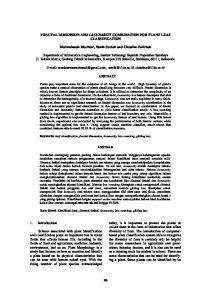
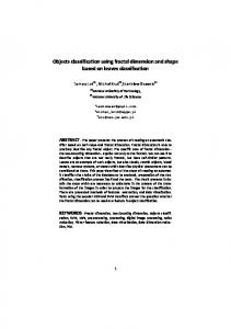
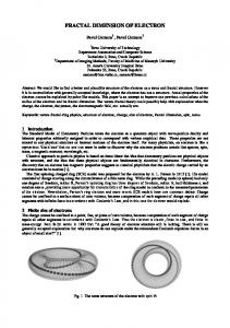
FIG. 1. Distribution of the radii of gyration of clusters containing more than 2000 particles: ~a! f 50.008, ~b! f 50.08. Log-log plots of two moments of the distribution at f 50.008: ~c! s 3 vs s 2 , ~d! s 4 vs s 2 .

be measured experimentally by scattering, this is the standard approach used to evaluate the fractal dimension of monodisperse systems. These two ways to evaluate d f , either from g(r) or from S(q), have been exploited repeatedly in the literature @2,23– 25#.

number of particles in cluster s entering in Eq. ~8!. Therea fore, the moments s p should vary as N i p where a p 5p/d f @16#. To determine the exponent a p , we search for the ratio of the logarithms of two moments of different order. If the moments s p , s q really have a scaling behavior, then the slope will be equal to p/q. Otherwise, the slope will show deviations from this value indicating a multiscaling regime. Figures 1~c! and 1~d! illustrate the ratios p/q5 23 and 42 for the sample at f 50.008. In Table I we give the values of the slope of similar graphs for several p,q ratios and for two concentrations. As is very clear from these results, the aggregates are indeed fractal objects. IV. THE FRACTAL DIMENSION FROM SINGLE CLUSTERS

As mentioned in Sec. II, clusters have been catalogued by size. For each of the six size sets we compute an averaged

III. SELF-SIMILARITY OF DLCA AGGREGATES

One of the features that would assure the validity of the two methods to obtain the fractal dimension described in the previous section is that the aggregates in the flocculation limit of a DLCA reaction would display simple scaling. If this is the case, then only one fractal dimension is enough to describe the fractal characteristics of the aggregates. Our statistical study of the scaling properties of the DLCA aggregates is inspired by the recent method of Mandelbrot et al. @15#. First we generate the distribution of radii of gyration of a sample of aggregates containing all the clusters with more than 2000 particles collected from the 50 simulations. This distribution is shown in Figs. 1~a! and 1~b! for two concentrations: f 50.008 and f 50.08. The moments of this distribution are defined by

s p~ R gi ! 5

1 ni

ni

(

s51

u R gi 2 ^ R g&u p, s

~8!

FIG. 2. Calculated averaged ^ g cluster(r) & ~circles! of clusters with 3001–3500 particles at f 50.01. The continuous line corresponds to ~a! the stretched exponential of Eq. ~6! with parameters from Table II, and ~b! the Fisher-Burford approximation with paFB FB rameters d FB f 51.865, A 51.606, j 587.89.

STRUCTURE FUNCTION AND FRACTAL DIMENSION OF . . .

57

4523

TABLE II. Values of d f obtained from ^ g cluster(r) & for various volume fractions f and various cluster size bins. Fractal dimension values from Ref. @8# are included for comparison. Also reported are the best values of the parameters in Eq. ~6!, obtained from the simulations.

f d f ~Ref. @8#! bin 3000

bin 3500

bin 4000

bin 4500

bin 5000

0.0065 df A j a df A j a df A j a df A j a df A j a

1.868 1.858 1.491 50.32 2.615 1.867 1.458 54.36 2.742 1.876 1.430 57.54 2.683 1.868 1.492 60.00 2.445 1.874 1.404 66.15 2.860

0.008

0.01

0.03

0.05

0.065

0.08

1.876 1.864 1.498 48.93 2.476 1.861 1.483 54.72 2.930 1.850 1.412 62.10 3.160 1.858 1.414 64.42 3.519 1.856 1.327 70.12 3.380

1.885 1.865 1.512 49.50 2.626 1.873 1.472 53.92 2.911 1.879 1.468 56.61 2.725 1.869 1.532 59.79 2.638 1.873 1.374 66.69 3.064

1.951 1.932 1.514 43.44 2.697 1.932 1.547 46.24 2.647 1.930 1.547 49.47 2.835 1.940 1.506 52.64 2.776 1.918 1.643 53.40 2.092

1.997 1.983 1.427 41.77 2.928 1.981 1.460 44.62 3.173 1.984 1.678 42.85 2.810 1.998 1.589 43.09 1.779 2.029 1.448 50.73 2.911

2.025 2.042 1.442 36.77 2.746 2.054 1.439 38.60 2.630 2.046 1.444 41.26 2.619 2.050 1.461 43.58 2.541 2.038 1.510 45.91 2.467

2.051 2.092 1.348 34.99 2.659 2.087 1.393 36.82 2.711 2.101 1.433 38.11 2.526 2.096 1.449 39.31 2.100 2.093 1.430 42.94 2.451

^ g cluster(r) & . Next, we perform a multiple parameter fit of Eq. ~6! to ^ g cluster(r) & to determine the values of the four param-

eters d f , A, a, and j for each size set and for each concentration. Figure 2~a! illustrates a typical fitted ^ g cluster(r) & for f 50.01 and size set 3001–3500 particles per cluster. The circles correspond to our simulations and the continuous line is the fitted function. As is evident, the fit is excellent. For this particular case the four parameters are d f 51.865, a 52.626, A51.512, and j 549.50. In addition, Fig. 2~b! shows the same simulation points as in Fig. 2~a! compared to the Fisher-Burford approximation of g(r) ~continuous line! FB with optimized parameters d FB f 51.865, A 51.606, and FB j 587.89. Although both approximations give the same fractal dimension, clearly the Fisher-Burford approximation does not reproduce the pair correlation function as closely as the stretched exponential. Table II contains the fitted values of these parameters for the other concentrations and size sets larger than 3000 particles. The first row of this table gives our predicted values of d f from Ref. @8#. As is clear, the value of d f is independent of the size set within the statistical error. It is also clear that the new results for the fractal dimension are in perfect agreement with our previous prediction, again within the statistical error. For small clusters the above analysis is not feasible. The reason is that when calculating ^ g cluster(r) & , many particles in the cluster surface contribute. Therefore the r d f 23 dependence is buried into the scaled decaying region. Care should be taken when an analysis involves early times during the aggregation because the majority of clusters are small. In the Appendix A we demonstrate that the structure function @Eq. ~7!# of the fitted g cluster(r) @Eq. ~6!# presents a length scale for which S(q) is linear in a log-log plot versus

q. This behavior is characteristic at relatively large values of q. In Fig. 3 we show the structure function corresponding to the g(r) in Fig. 2, obtained numerically from Eqs. ~3! and ~6!. This function displays a plateau for small q values, a shoulder at intermediate q values due to the stretched exponential, and the linear behavior at larger values of q. From the slope of the linear region, we can extract once again the value of d f . The fractal dimension obtained with this procedure is the same as the one carried in the corresponding g(r), as shown in Appendix A. Therefore, the values of d f in Table II are reobtained by this method. V. THE FRACTAL DIMENSION FROM THE WHOLE AGGREGATION BATH

For each of the seven concentrations we calculated the particle-particle correlation function @Eq. ~2!# of the whole

FIG. 3. S cluster(q) obtained by integration of the ^ g cluster(r) & of Fig. 2~a!.

4524

´ LEZ, AND BLAISTEN-BAROJAS LACH-HAB, GONZA

57

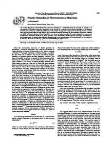
FIG. 4. Calculated g total(r) at the final time for one simulation with 138 240 particles and concentration f 50.01.

reaction box. This calculation was done at four different times during aggregation process and for five simulations. Figure 4 illustrates g total(r) from one of these simulations at the final time for f 50.01. The structure displayed by this function has already been reported @17,18#. The position of the minimum of this function is associated with half of the average length of the blobs that will be quenched in the infinite gel. At very short range, the main contribution to this function comes from pairs of particles within single clusters. However, at longer range, the individual clusters present the decay region associated to the stretched exponential. Therefore the function decays faster than at short range. In this intermediate range there are also pairs from different clusters that start to contribute significantly to the function. Somehow this effect washes out the sharp decay due to the finite size of the clusters, which is more pronounced at higher concentrations. At even longer range, the function includes many intercluster pairs that are responsible for the minimum and for the further increase of the g total(r). For the earlier times considered, the number of small clusters in the bath is large. Therefore, an analysis through the pair correlation function to obtain the d f is not adequate. This fact was already mentioned above. Figure 5 shows the log-log plot of the g total(r) for three concentrations at the final time. It is possible to extract d f from the limiting behavior of this function at short distances, and far from the minimum of the function. This is because at short distances g total(r) behaves as r d f 23 , similar to the correlation function of individual clusters. The continuous line in Figs. 5~a! and 5~b! shows the fit to obtain this dimension. For concentrations larger than f 50.05, when the final blob size is very small @17,18#, we find that the short-range region of g total(r) shrinks. An example is provided in Fig. 5~c! where it is clear that there are too few points to identify a linear behavior. In this case it is not possible to obtain d f with this method. The second column of Table III contains the fractal dimension from this method, averaged over the five simulations for each volume fraction up to f 50.05. Within the statistical error, d f displays the same behavior as a function of concentration as reported in Ref. @8#. In what concerns the method for obtaining the fractal dimension from the S total(q), there are serious problems for the finite concentrations used in this work. In Figs. 6~a! and 6~b! we are showing the S total(q) for the same simulations as in Figs. 5~a! and 5~b!. The structure function presents an ap-

FIG. 5. Log-log plot of g total(r) vs r at the final simulation time for three volume fractions: ~a! f 50.0065, ~b! f 50.01, ~c! f 50.065. The continuous line shows the region where a fit to obtain d f was possible.

TABLE III. Values of d f from g total(r) for various volume fractions. Also reported are the slopes in a log-log plot of the linear portion of S total(q) vs q.

f 0.0065 0.008 0.01 0.03 0.05 0.065 0.08

d f from g total(r)

uSlopeu from S total(q)

1.913 1.902 1.914 1.950 2.034

1.996 2.030 2.051 2.064

STRUCTURE FUNCTION AND FRACTAL DIMENSION OF . . .

57

4525

It is conceivable that for very dilute systems and long times, when well separated big clusters have aggregated, there would be a length scale for which g total(r) →g cluster(r). If this is the case, S total(q) would display the expected slope as in Eq. ~7!, in the correct length scale. VI. INVERSION OF THE SCATTERING FUNCTIONS

Unfortunately, the experimental way of obtaining the d f comes precisely from S total(q) via its relation to the normalized scattering intensity @26#. We have already mentioned that it is possible that in the limit of a very dilute system and for long times, S total(q) presents a slope proportioning the correct fractal dimension because of the presence of well separated big clusters in the DLCA regime. However, for higher concentrations there could be problems in obtaining the cluster fractal dimension from such log-log plots. One possible way to circumvent the problem is to extract the d f from the limit of g total(r) for small r’s. For this purpose, the experimentalists would need to consider the inversion of Eq. ~4!, in the form g total~ r,t ! 511

FIG. 6. Log-log plot of S total(q) vs q obtained from the g total(r) reported in Fig. 5: ~a! f 50.0065, ~b! f 50.01. The continuous line shows a linear region that does not lead to d f .

proximately linear behavior shown by the straight line between the points A and B. However, the values of the slopes obtained by a linear regression in that region should not be confused with the fractal dimension. In fact these slopes differ from the fractal dimension determined in Figs. 5~a! and 5~b!. The reason for this discrepancy is that S total(q) has a contribution not only from the short-range behavior r d f 23 of the g total(r), but also from the minimum and nearestneighboring cluster regions. The Fourier transform of this function g total(r) does not behave as Eq. ~7!. In fact, the length scale on which S total(q) roughly presents the linear behavior does not correspond to the short-range region of g total(r). The third column of Table III shows averages over the five simulations of the magnitude of the slope for those concentrations at which it was possible to find a straight line in the log-log plot of S total(q). As it is evident from the table, there are serious discrepancies between the values in the two columns.

1 2 p 2r i

E

np

0

@ S total~ q ! 21 # q sin~ qr i ! dq5

4r pri

1 2 p 2r r

E

`

0

q sin~ qr !@ S total~ q,t ! 21 # dq. ~9!

The problem that arises now is that experimentalists do not obtain the S(q) for all q’s to infinity, but only up to a maximum q defined by the maximum scattering angle of the scattering apparatus. Nonetheless, if we only want g total(r) defined at a set of discrete values of r, the restriction of an integration up to infinity can be spared. From now on we will consider that in Eqs. ~4! and ~9!, r, q, and r are in units of the particle diameter a 0 ~i.e., r 8 5r/a 0 →r, q 8 5qa 0 →q, and r 8 5 r a 30 → r !. Let D n 51/n (n51,2,3, . . . ) be the size of the bins in which the spatial coordinate r is divided. Let r i 5(2i21)/2n (i51,2,3, . . . ) be the centers of those intervals. Let g i be the approximations to g(r i ) such that, for all qP @ 0,n p # , the following discrete sum replaces Eq. ~4!: 4 pr q

`

( D n r i sin~ gr i !~ g i21 ! 5S total~ q ! 21.

i51

~10!

When the size of the subdivisions tends to zero, g i →g(r i ). In particular, although the g i ’s for r i ,1 need not be exactly zero, they should tend to that value when n→`. Using the above equation, we can calculate easily

( r j ~ g j 21 ! E0 j51 `

p /2

sin@ q ~ 2i21 !# sin@ q ~ 2 j21 !# dq5 r ~ g i 21 ! ,

~11!

where we have used

E

p /2

0

sin@ j ~ 2i21 !# sin@ j ~ 2 j21 !# d j 5

Then the approximation for g(r) at r i is

p d , 4 i, j

i, j integers>1 .

~12!

´ LEZ, AND BLAISTEN-BAROJAS LACH-HAB, GONZA

4526

g i 511

1 2 p 2r r i

E

np

0

q sin~ qr i !@ S total~ q ! 21 # dq.

As is well known @26#, the scattering vector q is related to the scattering angle u by the relation

q5

4p sin~ u /2! , l

~14!

where l is the wavelength of light used in the scattering apparatus. If we want an approximation of g(r) defined by the integer n in Eq. ~10!, then a 0 q max5np. Since the maximum value that the sine can take ~for backward scattering! is 1, then we should have ~15!

nl,4a 0 .

57

This last relation presents a restriction in the particle diameter that the system should fulfill in order to be able to approximately invert Eq. ~4! in the form of Eq. ~13!.

~13!

have shown that the S total(q) can be approximately inverted yielding an approximation for g(r) from where in turn the fractal dimension could be extracted. Experimentally S total(q) is obtained from the intensity function I total(q) only for monodisperse systems. An additional experimental restriction appears now in the form nl,4a 0 , where l is the wavelength of light used in the scattering apparatus and a 0 is the particle diameter. This restriction would force experimentalists to consider the aggregation of larger particles in order to obtain a better approximation to g(r). ACKNOWLEDGMENTS

E.B.B. acknowledges support from NSF Grant No. INT9502985 for international travel expenses, and from the Institute for Computational Sciences and Informatics for financial support to M.L. and for supplying most of the computing time used in this work. A.E.G. acknowledges support from CONACYT Grant Nos. 4906-E, 3165-PE, and E120.1381, and from Cray-UNAM Grant No. SC-006096.

VII. CONCLUSION

We have demonstrated that for the finite concentrations used in this work we recover the concentration dependence of the fractal dimension of the DLCA aggregates of monodisperse particles, which we reported in a previous publication @8# using another method. In the present work we have obtained the d f via the particle-particle correlation functions of single clusters and of the whole aggregation bath. In the latter case, it was necessary to consider the limiting slope of g total(r) for small r in order to exclude the contributions from the other clusters in the system. We have also obtained the d f from the structure function of single clusters S cluster(q), defined in Eq. ~3! and, as shown in Appendix A, it gives exactly the same values as those obtained from g cluster(r). We have seen, however, that the S total(q) fails to produce linear slopes on log-log plots with the correct fractal dimension in the concentration range studied. It was observed that the discrepancy arose from contributions to S total(q) coming from the minimum and nearest-neighbor cluster length regions of g total(r) in Eq. ~4!. Nevertheless, we

In this appendix we show that the structure function for single clusters behaves as S cluster(q);q 2d f , for sufficiently large q. In the Fisher-Burford representation of g cluster(r), the proof is done analytically, while for the stretched exponential case, it is done numerically. If the Fisher-Burford expression for g cluster(r) is used in Eq. ~3! then FB

S cluster~ q ! 5B FBq 2d f

E

`

FB

rdf

22

0

FB

~ sin r ! e 2r/q j dr,

~A1!

where an appropriate change of variables has been performed and where B FB includes all numerical factors independent of q and j FB. This integral is found in the standard tables @27#, with the result

G ~ d FB f 21 !

FB

S cluster~ q ! 5B FBq 2d f

APPENDIX A

FB

„111/~ q j FB! 2 …~ d f

21 ! /2

FB sin@~ d FB f 21 ! arctan q j # .

~A2!

An expansion in powers of 1/q j FB up to the first order, leads to

FB

FB 2d f

S cluster~ q ! 5B q

G ~ d FB f 21 !

F S

D

S

d FB p FB p FB f 21 sin cos ~ d f 21 ! 2 ~ d f 21 ! 2 q j FB 2

DG

,

~A3!

STRUCTURE FUNCTION AND FRACTAL DIMENSION OF . . .

57

FB assuming that d FB f Þ2. For d f 52 there is no first order term and the correction is second order. For the case q j FB@1,

S

D

S cluster~ q ! 5Bq 2d f

4527

E

qj

0

r d f 22 ~ sin r ! dr.

~A6!

This integral does not appear in the standard tables of integrals for aÞ1. For a51, it reduces to Eq. ~A1! and for q j @1 becomes independent of q. On the other hand, for a @1 the exponential factor becomes a step function with the value of 1 for r,q j and zero for r.q j . This effectively cuts the integral off at the upper limit q j :

The integral * `0 r d f 22 sin r dr converges very slowly for 1,d f ,2 and diverges for d f >2 @27#. Therefore the integral in Eq. ~A6! becomes independent of q for d f ,2 and very large q j . However, this integral depends on q for d f >2. Consequently, there should be a crossover value of a below which the integral in Eq. ~A5! for d f .2 is independent of q and above which depends on q. It becomes imperative to test the dependency of this integral on q for the d f ’s and a’s that we have obtained. A look at Table II shows that the values of d f involved are in the range 1.85,d f ,2.10, while the values of a are mainly between 2.50,a,3.25. We have performed numerically the integral for the following q j values: 2 n 3100 with n50,1, . . . ,12. The values of d f used were 1.80