Structure induction by lossless graph compression

Structure induction by lossless graph compression Leonid Peshkin Center for Biomedical Informatics Harvard Medical School Boston, MA 02115, USA [email protected]

arXiv:cs/0703132v1 [cs.DS] 27 Mar 2007

Abstract This work is motivated by the necessity to automate the discovery of structure in vast and evergrowing collection of relational data commonly represented as graphs, for example genomic networks. A novel algorithm, dubbed Graphitour, for structure induction by lossless graph compression is presented and illustrated by a clear and broadly known case of nested structure in a DNA molecule. This work extends to graphs some well established approaches to grammatical inference previously applied only to strings. The bottom-up graph compression problem is related to the maximum cardinality (non-bipartite) maximum cardinality matching problem. The algorithm accepts a variety of graph types including directed graphs and graphs with labeled nodes and arcs. The resulting structure could be used for representation and classification of graphs.

1

Introduction

The explosive growth of relational data, for example data about genes, drug molecules and proteins, their functions and interactions, necessitates efficient mathematical algorithms and software tools to extract meaningful generalizations. There is a large body of literature on the subject coming from a variety of disciplines from Theoretical Computer Science to Computational Chemistry. However, one fundametal issue has so far remained unaddressed. Given a multi-level nested network of relations, such as a complex molecule, or a protein-protein interaction network, how can its structure be inferred from first principles. This paper is meant to fill this surprising gap in automated data processing. Let us illustrate the purpose of this method through the description of DNA molecular structure, the way most of us learned it from a textbook or in class. • The DNA molecule is a double chain made of four kinds of nucleotides: A, T, G, C; • Each of these is composed of two parts: one part—backbone—is identical among all the nucleotides (neglecting the difference between ribose and 2’-deoxyribose), another—heterocyclic base—is nucleotide-specific; • The backbone consists of sugar and phosphate; • The heterocyclic bases (C,T-pyrimidines; A,G-purines) all contain a pyrimidine ring; • The components can be further reduced to individual atoms and covalent bonds. This way of description is not unique, and may be altered according to the desired level of detail, but crucially, it is a hieararchical description of the whole as a structure built from identifiable and repetitive subcomponents. The picture of this beautiful multi-level hierarchy has emerged after

Figure 1. A graph with repetative structure and a corresponding grammar. years of bio-chemical discovery by scientists who gradually applied their natural abstraction and generalization abilities. Hence, structural elements in this hierarchy also make functional sense from bio-chemical point of view. The properties of hierarchical description are formally well-studied and applied in other scientific domains, such as linguistics and computer science. It is viewed as the result of a rule-driven generative process, which combines a finite set of undecomposable elements—terminal symbols— into novel complex objects—non-terminal symbols, which can be combined in turn to produce the next level of description. The rules and symbols on which the process operates are determined by a grammar and the process itself is termed a grammatical derivation. In the case of the DNA molecule above, the chemical elements correspond to terminal symbols. They are assembled into non-terminal symbols, i.e. compounds, according to some set of production rules defined by chemical properties. Now, imagine receiving an alternative description of the same object, stripped off of any domain knowledge and context, simply as an enormous list of objects and binary relations on objects, corresponding to thousands of atoms and covalent bonds. Such a list would remain completely incomprehensible to a human mind, along with any repetitive hierarchical structure present in it. Discovering a hierarchy of nested elements without any prior knowledge of a kind, size and frequency of these constitutes a formidable challenge. Remarkably, this is precisely the challenge which is undertaken by contemporary scientists trying to make sense of data, mounting up from small fragments, like protein interaction networks, regulatory and metabolic pathways, small molecule repositories, homology networks, etc. Our goal is to be able to approach such tasks in an automated fashion. Figure 1 illustrates the kind of induction we describe in this paper on a trivial example. We will use this as a running example throughout the paper, leaving more rigorous mathematical formulation out for the purpose of clarity and wider accessibility. To the left is a graph which contains repetitive structure. Let us imagine for a moment that the human researcher is not smart enough to comprehend a 6-node graph and find an explanatory layout. Thus, we would want to automatically translate such a graph into the graph grammar on the right. The graph grammar consist of two productions. The first expands a starting representation—a degenerate graph of a single node ”S”—into a graph connecting two nodes of the same type ”S1”. The second additionally defines a node ”S1” as a fully connected triple. Formal description of the relational data of such kind is known as graphs, while the hierarchical nested structures of such kind are described by graph grammars. It is outside the scope of this paper to survey a vast literature in the field of graph grammars; please refer to a book by G. Rozenberg [3]

Table 1. Generalized string compression algorithm. Input: initial string; Initialize: empty grammar; Loop: Make a single left-to-right tour of the string, collecting sub-string statistics; Introduce a new non-terminal symbol (compound) into the grammar, which agglomerates some sub-string of terminal and non-terminal symbols; Substitute all occurrences of a new compound; Until no compression possible; Output: compressed string & induced grammar;

for extensive overview. It suffices to say that this field is mostly concerned with the transformation of the graphs, or parsing, i.e. explaining away a graph according to some known graph grammar, rather than with inducing such grammar from raw data. The closest work related to the ideas presented here is due to D. Cook, L. Holder and their colleagues (e.g. see [2] and several follow-up papers). Their work however is not concerned with inducing a structure from given graph data. Rather, they induce a flat, context-free grammar, possibly with recursion, which is not only capable of, but is also bound to, generate objects not included in the original data. Thus, their approach defies the relation to compression exploited here. Moreover, the authors present the negative result of running their SUBDUE algorithm on just the kind of biological data we successfully use in this paper. Another remotely similar work is by Stolke [10] in application to inducing hidden Markov models. There are many other works attempting to induce structure from relational data or compress graphs, but none seem to relate closely to the method considered here. Our method builds on the parallels between understanding and compression. Indeed, to understand some phenomenon from the raw data means to find some repetitive pattern and hierarchical structure, which in turn could be exploited to re-encode the data in a compact way. This work extends to graphs some well established approaches to grammatical inference previously applied only to strings. Two methods particularly worth mentioning in this context for grammar induction on sequences are Sequitour [6] and ADIOS [8]. We also take inspiration from a wealth of sequence compression algorithms, often unknowingly run daily by all computer users in a form of archival software like pkzip in Unix or expand for Mac OS X. Let us briefly convey the intuition behind such algorithms, many of which are surveyed by Lehman and Shelat [1]. Although quite different in detail, all algorithms share common principles and have very similar compression ratio and computational complexity bounds. First, one has to remember that all such compression/discovery algorithms are bound to be heuristics, since finding the best compression is related to the so-called Kolmogorov complexity and is provably hard [1]. These heuristics are in turn related to the MDL (Minimum Description Length) principle, and work in the way described by Table 1. Naturally, the difference is in how exactly statistics are used to pick which substring will be substituted by a new compound symbol. In some cases, a greedy strategy is used (see e.g. Apostolico & Lonardi [7]), i.e. the substitution which will maximally reduce the size of the encoding at the current step is picked; in other cases, a simple first-come-first-served principle is used and any repetition is immediately eliminated (see e.g. Nevill-Manning & Witten [6]).

Table 2. Graphitour: graph compression algorithm. Input: initial graph: lists of (labeled) nodes and edges; Initialize: empty graph grammar, empty edge lexicon; Build edge lexicon: make a single tour of the graph, register the type of each edge according to the edge label and types of its end nodes; collect type statistics; Loop: Loop through edge types For a sub-graph induced by each edge type solve an instance of maximum cardinality matching problem, which yields a number and list of edges that could be abstracted; Pick an edge type which corresponds to the highest count; Introduce a new hyper-node for the chosen edge type into the graph grammar; Loop through edge occurrences of a chosen type throughout the graph; Substitute an occurrence of the edge type with a hyper-node; Loop through all edges incident to the end nodes of a given edge; Substitute edges and introduce new edge types into edge lexicon; Until no compression possible; Output: compressed graph & induced graph grammar;

Extending these methods to a graph structure turns out to be non-trivial for several reasons. First, maintaining a lexicon of strings and looking up entries is quite different for graphs. Second, directly extending the greedy approach [7] fails due to inherent non-linear entity interactions in a graph.

2

Algorithm

The algorithm we present is dubbed ”Graphitour” to acknowledge a strong influence of the Sequitour algorithm [6] for discovering the hierarchical structure in sequences. In particular, Graphitour just like Sequitour restricts the set of candidate structures to bigrams, which allows it to eliminate a rather costly lexicon lookup procedure, as well as sub-graph isomorphism resolution, which is NPhard. Note that Graphitour in principle admits labeled nodes and edges, particularly since unlabeled graphs turn into labeled at the first iteration of the algorithm. The algorithm is presented in Table 2 and best understood through the illustration of every step on a trivial example of Figure 2 as described below. Figure 2 presents an imaginary small molecule with two types of nodes-atoms: ”H” and ”C”. Each edge is typed according to its end nodes. The first iteration is to tour the graph making a lexicon of edge types and corresponding frequencies. Figure 2 shows three kinds of edges we observe: ”C-C”, ”C-H” and ”H-H” with corresponding counts. The next step is to select which kind of edge will be abstracted into a (hyper)node corresponding to a new compound element. A greedy choice would have picked the most frequent type of edge, disregarding potential conflicts due to shared node interactions. Instead Graphitour proceeds by decomposing the graph into three graphs each containing only edges of one type, which is illustrated by Figure 3, and counting how many edges of each type could be abstracted, taking into account node interactions.

Figure 2. left: A simple graph with labeled nodes corresponding to an imaginary small molecule and a corresponding sample edge lexicon with type frequency counts. right: Non-bipartite maximum cardinality matching. One of the key contributions of the algorithm described here is in relating the graph grammar induction to the maximum cardinality non-bipartite matching problem for which there is a polynomial complexity algorithm due to Gabow [4]. The problem is formulated as follows: given a graph, find the largest set of edges, such that no two edges share a node. Figure 2.right illustrates this on an arbitrary non-bipartite graph. Dashed edges represent a valid matching. The description and implementation of the algorithm is quite technically involved and does not belong to the scope of this paper. Note that while applying Gabow’s elegant algorithm essentially allows us to extend the horizon from one-step-look-ahead greedy to two-step-look-ahead, the bottom-up abstraction process still remains a greedy heuristic. Only one partial graph of Figure 3, containg ”C-H” edges, makes a non-degenerate case for a maximal non-bipartite matching since edges interact at the node ”H”, obviously returning only two out of four edges subject to abstraction, marked with an oval shape on the figure. A new entry is made into the lexicon, called ”HC” which corresponds to an abstracted edge, as illustrated by two steps going right to left in Figure 4. The leftmost sub-figure of Figure 4 is an input for the next iteration of the algorithm, which detects the new repetitive compound: edge ”HC-C”, which is abstracted again, ultimately producing a graph grammar shown in the Figure 1 on the right. Note that as the algorithm iterates through the graph, intermediate structures get merged with the higher level structures.

Figure 3. A graph decomposition into subgraphs induced by edges of different type.

Figure 4. A sequence of abstraction steps, right to left: a new entry is made into the lexicon, called ”HC” which corresponds to an abstracted edge.

3

Results

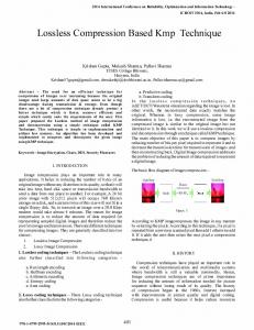
In this section we take a closer look at the results of running Graphitour on raw data obtained from a PDB file of a DNA molecule by stripping off all the information except for the list of atoms and the list of of covalent bonds. To simplify the representation of results, hydrogen atoms and corresponding edges were removed from the graph. Additionally, to support the symmetry, we artificially linked the DNA into a loop by extra bonds from 3’ to 5’ ends. The resulting list of 776 nodes and 2328 edges in the incidence matrix is presented as input to Graphitour and is depicted in Figure 5. Figure 6.left and 6.right show two sample non-terminals from the actual output from the Graphitour software, illustrating the discovery of basic DNA elements. 238 224

228 237

226

232

236 233

243

211

212 218 210

234

213

214

219

318

316

230

241

217 208

320

315

314

223

229

235

242

220

221 231

240

225

227 222

239 317

215

209

158

319

313

157

216

207 321

322

204

206 155

203

205

340

338

160

159

156

339 312

161

154

311

153

307

189

336

310

337

341 152 188

324

306 308

303

335

342

343

325

305 309

323

187

200

333

329

201

290

291

136 145 193

330

165

182

288

142

346

127

168

197 345

172

126

347

298

299

132 129 128

297

285

274

130

143

167

171

344 300

125

173

273

281

135

131

144

275

280

166 169

196

331 296

286 278

134 133

170

194 294 293

164

195 198

292

276 277

141

199 332

295

287 279

137 146

162 181

202 328

289

150

183

192

327

139

163 184

326

147

149

191

138 140

185

334

301

148

151

190 186

304

302

282

348 284

174

175

123 122

180

124

272 268

283

271

350

269

356

357

270

109

349 176

179

267 354 355 266

108

177

351

358

265

110

352

359

367

114

106

105

178

111

104

103

264

112

107 115

365

363 263

366

101

361

121

362 262

113

353 364

360

117

102

368

260

116

88

120

261 89

92

369

249

87

93

118

119 77

248 246

244

86

382

374

73

98 397

259

389

391

254

66

81

377

386

74

72

67

381

379

390

395

396

79

80

380

399

253

75

99

97

388

78

83

376

385 252

76

84

384

375

373 398

100

95

383

372 387

247 251

85

94

96

371

245

250

90

91

370

65

82

68

69 71

378

400

258

255

401

394

404

63

1

392

402

256

2 61 407

405

3 4

406

408

5 6

8

48 39 41

49

16 413

18

51 26

23 446

447

431

450

29

473 467

433

478

451

454 453

481

472

435

439

468

455

438

470

436 456

475

480

469

32

33

486

35

466

437

30 37

476

452

440

31

479

474

465

441

55

38

477

434 445

54

28

430

444

53 56

449

443 442

57

27

432

429

52

50

14

428

418

40

15

448

427 425

24

22

13

424

414 417

45

19

412

415

25

21

426 416 419

46 44

17

12

420

60

43

20

9

423

42

7

10 410

411

59

58 47

11 409

422

421

70

64

62 393

403

257

482

34

36

471 485 483

457

464 463

484

458 462

461

459 460

Figure 5. Layout of original graph corresponding to a small DNA molecule.

Structure 2152 of type 263, depth 5

Structure 1984 of type 143, depth 5

C

O O

N N

P O

C

O

C C N

C

C C O

C N N

C

O

C

Figure 6. left: The compound object induced by the Graphitour algorithm, which corresponds to the base of Guanine. All four DNA bases were identified as nonterminal nodes in the resulting graph grammar. right: The compound object induced by the Graphitour algorithm, which corresponds to the backbone of the molecule: phosphate and sugar Figure 6.left shows the compound object induced by the Graphitour algorithm, which corresponds to the base of Guanine. All four DNA bases were identified as non-terminal nodes in the resulting graph grammar. This particular structure is identified as a non-terminal by the number 2152 in a list of non-terminals and described as type 263 in the lexicon of compounds. It is at the depth 5 in the hierarchy tree of the whole graph, being joined with the corresponding backbone phosphate & sugar one level higher in the upstream; subsequently joined with the complete nucleotide adjacent to it, and so forth. Figure 6.right shows the compound object induced by the Graphitour algorithm, which corresponds to the backbone of the molecule: joined phosphate and sugar. This particular structure is identified as a non-terminal by the number 1984 in a list of non-terminals and described as type 143 in the lexicon of compounds. It is at the depth 5 in the hierarchy tree of the whole graph, same depth as compound in Figure 6.left which makes sense. Note that although the number of lexicon entries is over a hundred, the vast majority of numbers were only used for intermediate entries, which got merged into composite elements. There is no reusing of the available lexicon slots. Such re-use could give some extra compression efficiency (compare to Sequitour [6]). The resulting lexicon is small and all the entries in the final lexicon are biologically relevant compounds. Graphitour actually discovers the hierarchical structure corresponding to the kind of zoom-in hierarchical description we gave in the introduction. The algorithm identifies all of these structural elements without exception and does not select any elements which would not make biological sense. The significance of such result might not be immediately clear if one does not take into account that the algorithm does not have any background knowledge, any initial bias, nothing at all except for the list of nodes and edges. As an example of a rather different application domain, we tried Graphitour on escherichia coli transcriptional regulation network, since it is one of the well known attempts to discover ”network motifs” or building blocks in a graph as over-represented sub-graphs by Alon et al. [9]. In this network there are 423 nodes corresponding to the genes or groups of genes jointly transcribed

flgMN

malZ

tsr flhBAE malEFG malPQ

fliAZY

malT

fliC flgKL

malS

fliDST

malK_lamB_malM

livJ

kbl_tdh

tarTapcheRBYZ

nycA

hypA

ilvIH

sdaA

rpoN

lrp serA

gltBDF

atoC atoDAB

lysU

livKHMGF oppABCDF

atoDAE

Figure 7. Compositional elements of E.coli regulatory network. (operons). Edges correspond to the 577 known interactions: each edge is directed from an operon that encodes a transcription factor to an operon that it directly regulates. For more information on the biological significance of the motif discovery in regulatory networks we refer you to the cited paper [9] and supplementary materials at the Nature Internet site. Alon et al. find that much of the network could be composed of repeated appearances of three highly significant motifs, that is a sub-graph, of a fixed topology, in which nodes are instantiated with different node labels. One example is what they call a feedforward loop X → Y → Z combined with X → Z, where X, Y, Z are instantiated by particular genes. In order to compare to the results of Alon et al. we label nodes simply according to cardinality, omitting gene identities, and take into account directionality of the edges. No hierarchical structure or feedforward loops were distilled from the data. Rather, Graphitour curiously disassembled the network back into the sets of star-like components as illustrated by Figure 7, which ought to have been initially put together to create such network. It leaves open the question of what is a useful definition of a network component in biological networks, if not the one requiring the most parsimonious description of the network.

4

Implementation

The implementation of this algorithm was done in Matlab version 6.5 and relies on two other important components also developed by the author. The first is a maximum cardinality non-bipartite matching algorithm by Gabow [4] implemented by the author in Matlab. The other component is a graph layout and plotting routine. Representing the original input graph as well as the resulting graph grammar is a challenging task and is well outside the scope of this paper. For the purposes of this study we took advantage of existing graph layout package from AT&T called GraphViz [5]. The author has also developed a library for general Matlab-GraphViz interaction, i.e. converting the graph structure into GraphViz format and converting the layout back into Matlab format for visualization from within Matlab. Supplementary materials available upon request contain several screen-shots of executing the algorithm on various sample graphs, including regular rectangular and hexagonal grids, synthetic floor plans and trees with repetitive nested branch structure. These are meant to both illustrate the details of our approach and provide a better intuition of iterative analysis.

5

Discussion

We presented a novel algorithm for the induction of hierarchical structure in labeled graphs and demonstrated successful induction of a multi-level structure of a DNA molecule from raw data—a PDB file stripped down to the list of atoms and covalent bonds. The significance of this result is that the hierarchical structure inherent in a multi-level nested network can indeed be inferred from first principles with no domain knowledge or context required. It is particularly surprising that the result is obtained in the absence of any kind of functional information on the structural units. Thus, Graphitour can automatically uncover the structure of unknown complex molecules and “suggest” functional units to human investigators. While, there is no universal way to decide which components of the resulting structure are ”important” across all domains and data, frequencies of occurrence is one natural indicator. One exciting area of application which would naturally benefit from Graphitour is automated drug discovery. Re-encoding large lists of small molecules from PBD-like format into grammarlike representation would allow for a very efficient candidate filtering at the top levels of hierarchy with the added benefit of creating structural descriptors to be matched to functional features with machine learning approaches. Analysis of proteins benefits from the same multi-level repetition of structure as DNA, and Graphitour gets similar results for individual peptides. Analyzing a large set of protein structures together is our work in progress. The hope is to reconstruct some of the domain nomenclature and possibly re-define the hierarchy of the domain assembly. The current version of the Graphitour corresponds to a so-called non-lossy or lossless compression. This guarantees that the algorithm will induce a grammar corresponding precisely to the input data, without over- or under-generating. The drawback of this approach is that the algorithm is sensitive to noise and has rather poor abstraction properties. Future work would require developing lossy compression variants, based on the approximation of description length minimization. Finally, it would be quite interesting to analyze the outcome of the algorithm from a cognitive plausibility point of view, that is to compare structures found by human investigator to these descovered by the algorithm on various application examples.

Acknowledgement A substantial part of this work was done while the author was visiting MIT CSAIL with Prof. Leslie Kaelbling, supported by the DARPA through the Department of the Interior, NBC, Acquisition Services Division, under Contract No. NBCHD030010.

References [1] E. Lehman, and A. Shelat, ”Approximations algorithms for grammar-based compression”, In Thirteenth Annual Symposium on Discrete Algorithms (SODA), 2002. [2] D. Cook, and L. Holder, ”Substructure Discovery Using Minimum Description Length and Background Knowledge”, Journal of Artificial Intelligence Research, 1994, 1, pp. 231-255. [3] G. Rozenberg (Ed.) ”Handbook of graph grammars and computing by graph transformation: Foundations”, World Scientific Publishing Company, 1997. [4] H. Gabow, ”Implementation of Algorithms for Maximum Matching on Nonbipartite Graphs”, Ph.D. thesis, Stanford University, 1973. [5] J. Ellson, E. Gansner, E. Koutsofios, S. North, and G. Woodhull, ”Graphviz and Dynagraph - Static and Dynamic Graph Drawing Tools”, Graph Drawing Software, Springer Verlag, 2003. [6] C. Nevill-Manning, and I. Witten, ”Identifying Hierarchical Structure in Sequences: A linear-time algorithm”, Journal of Artificial Intelligence Research, 1997, 7, pp. 67-82. [7] A. Apostolico, and S. Lonardi, ”Off-line Compression by Greedy Textual Substitution”, Proceedings of the IEEE DCC Data Compression Conference, 2000, 88, pp. 1733-44. [8] Z. Solan, D. Horn, I. Ruppin, and S. Edelman, ”Unsupervised learning of natural languages”, Proceedings of the National Academy of Sciences, 2005, 102, pp. 11629–34. [9] O. Shen-Orr, R. Milo, S. Mangan, and U. Alon, ”Network motifs in the transcriptional regulation network of Escherichia coli”, Nature Genetics, 2002, 31, pp. 64-68. [10] A. Stolcke, and S. Omoho, ”Hidden Markov model induction by Bayesian model merging”, Advances in Neural Information Processing Systems, 1993, 5, pp. 11–18.

Structure 2165 of type 242, depth 8 O

O

P

O

O C N

C C

N C

N

O

C

N

C

N

C C

C

C C

O

N

N C

C O

O

N P O O

C

C

O C

O C

C

C

Structure 1934 of type 137, depth 5

O

N

C

C N

C C

N

Top−level resulting graph. Labels are non−terminal types. Click to examine. 263.2154 3. 230

3. 473 28.1209 263.2152

234.2121 189.2043 96.1772

137.1934 164.1992

240.2127 240.2133

185.2029 247.2135 185.2026 189.2037

185.2035

214.2090 94.1786

214.2081 247.2142 185.2032

212.2078 102.1820 178.2017 223.2101 80.1683

2. 77

110.1843 223.2106 160.1976

164.1984

86.1714

142.1941

137.1922

189.2041 67.1575

275.2167 28.1044 196.2046

275.2165

196.2050

Top−level resulting graph. Labels are non−terminal types. Click to examine. 155.1996 229.2133

3. 230 28.1119

153.1987

244.2150 155.1997

159.2006 211.2111 126.1914

153.1988

197.2084

94.1789

211.2112

137.1950

161.2018 195.2079

161.2012 195.2078

197.2085 97.1799

28.1077

97.1801 196.2080

196.2081

159.2002 197.2083

244.2152 28.1065 159.2008 155.1998

197.2082 161.2010 137.1949

137.1955 155.1995 94.1775 198.2096 210.2110

3. 473

198.2086 229.2132 155.1994