Structure Inference of Bayesian Networks from Data

Structure Inference of Bayesian Networks from Data: A New Approach Based on Generalized Conditional Entropy Dan A. Simovici∗ , Saaid Baraty∗ ∗

Univ. of Massachusetts Boston, Massachusetts 02125, USA {dsim,sbaraty}@cs.umb.edu

Abstract. We propose a novel algorithm for extracting the structure of a Bayesian network from a dataset. Our approach is based on generalized conditional entropies, a parametric family of entropies that extends the usual Shannon conditional entropy. Our results indicate that with an appropriate choice of a generalized conditional entropy we obtain Bayesian networks that have superior scores compared to similar structures obtained by classical inference methods.

1

Introduction

A Bayesian Belief Network (BBN) structure is a directed acyclic graph which represents probabilistic dependencies among a set of random variables. Inducing a BBN structure for the set of attributes of a dataset is a well known problem and a challenging one due to enormity of the search space. The number of possible BBN structures grows super-exponentially with respect to the number of the nodes. In Cooper and Herskovits (1993), where the K2 heuristic algorithm is introduced, a measure of the quality of the structure is derived based on its posterior probability in presence of a dataset. An alternative approach to compute a BBN structure is based on the Minimum Description Length principle (MDL) first introduced in Rissanen (1978). The algorithms of Lam and Bacchus (1994) and Suzuki (1999) are derived from this principle. We propose a new approach to inducing BBN structures from datasets based on the notion of β-generalized entropy (β-GE) and its corresponding β-generalized conditional entropy (βGCE) introduced in Havrda and Charvat (1967) and axiomatized in Simovici and Jaroszewicz (2002) as a one-parameter family of functions defined on partitions (or probability distributions). The flexibility that ensues allows us to generate BBNs with better scores than published results. One important advantage of our approach is that, unlike Cooper and Herskovits (1993) it is not based on any distributional assumption for developing the formula.

2

Generalized Entropy and Structure Inference

The set of partitions of a set S is denoted by PART(S). The trace of a partition π on a subset T of S is the partition πT = {T ∩ Bi | i ∈ I and T ∩ Bi 6= ∅} of T . The usual order between set partitions is denoted by “≤”. It is well-known that (PART(S), ≤) is a bounded

Inference of Bayesian Networks

lattice. The infimum of two partitions π and π 0 = {Bj |j ∈ J} on S, denoted with π ∧ π 0 , is the partition {Bi ∩ Bj |i ∈ I, j ∈ J, Bi ∩ Bj 6= ∅} on S . The least element of this lattice is the partition αS = {{s} | s ∈ S}; the largest is the partition ωS = {S}. The notion of generalized entropy or β-entropy was introduced in Havrda and Charvat (1967) and axiomatized for partitions in Simovici and Jaroszewicz (2002). If S is a finite set and µ π = {B1 , . . . , Bm } ¶ is a partition of S, the β-entropy of π is the number Hβ (π) = ´β ³ P m |B | 1 for β > 1. The Shannon entropy is obtained as limβ→1 Hβ (π). 1 − i=1 |S|i 1−21−β For β ≥ 1 the function Hβ : PART(S) −→ R≥0 is anti-monotonic. Thus, Hβ (π) ≤ 1−nβ−1 Hβ (αS ) = (21−β , where n = |S|. −1)·nβ−1 Let π, σ ∈ PART(S) be two partitions, where π = {B1 , . . . , Bm } and σ = {C1 , . . . , Cn }. Pn ³ |C | ´β The β-conditional entropy of π and σ is Hβ (π|σ) = j=1 |S|j Hβ (πCj ). It is immediate that Hβ (π|ωS ) = Hβ (π) and that H(π|αS ) = 0. Also, in Simovici and Jaroszewicz (2006) it is shown that Hβ (π|σ) = Hβ (π ∧ σ) − Hβ (σ), a property that extends the similar property of Shannon entropy. When β ≥ 1 the β-GCE is dually anti-monotonic with respect to its first argument and is monotonic with respect to its second argument. Moreover, we have Hβ (π|σ) ≤ Hβ (π). Let D be a dataset with set of attributes Attr(D). The domain of attribute Ai ∈ Attr(D) is Dom(Ai ). The projection of a tuple t ∈ D on X is the restriction t[X] of t to the set X. The set of attributes X defines a partition π X on D, which groups together the tuples that have the equal projections on X. Let A be an attribute and let X be set of parents for A, where Dom(A) = {v1 , v2 , ..., vn } Q and Dom(X) = B∈X Dom(B) = {u1 , u2 , ..., um }. Define pij = P (t[A] = vi |t[X] = uj ). Pn β 1 We have nβ−1 ≤ i=1 pij ≤ 1 for β ≥ 1. X is considered as a “good” parent set for A if knowingPthe its value enables us to predict the value of A with a high probability, that n β is, if aj = for every j where P (t[X] = uj ) is sufficiently large. i=1 pij is close to 1 Pm Clearly, X is a “perfect” parent if j=1 aj = m. The β-GCE captures exactly this parenthood quality measure. Indeed, suppose that π A = {Bi |1 ≤ i ≤ n} and π X = {Cj |1 ≤ j ≤ m}, where for t ∈ Bi we have t[A] = vi , and for s ∈ Cj we have s[X] = uj . |Bi ∩Cj | Then, pij = P (t[A] = vi |t[X] = uj ) = P (t ∈ Bi |t ∈ Cj ) = |C , which implies j| P m 1 A X β A X Hβ (π |π ) = 1−21−β j=1 P (Cj ) (1 − aj ). Thus, minimizing Hβ (π |π ) amounts to reducing the values of (1 − aj ) as much as possible for those j’s where |Cj | is large, that is, P (Cj ) = P (t[X] = uj ) is non-trivial. We refer to quantity Hβ (π A |π X ) as the entropy of node A in presence of set X. However, even if X = argminX (Hβ (π A |π X )), the value of the minimum itself may be too high to insure good predictability. An alternative is to meaH (π A |π X ) sure the reduction of entropy of node A as a result of presence of set X as βHβ (πA ) . Since H (π A |π X )

0 ≤ Hβ (π A |π X ) ≤ Hβ (π A ) we have 0 ≤ βHβ (πA ) ≤ 1. If X is a perfect parent set for A, then aj = 1 for 1 ≤ j ≤ m, so Hβ (π A |π X ) = 0. Let ² ∈ [0, 1] be a number referred to as prediction threshold. We regard X as a ²-suitable H (π A |π X )

parent of A if βHβ (πA ) ≤ ². To avoid cycles in the network we start from a sequence of attributes A1 , A2 , ..., Ap and we seek the set of parents for Ai in the set Φ(Ai ) = {A1 , . . . , Ai−1 }, a frequent assumption RNTI - X -

D. A. Simovici and S. Baraty

F IG . 1 – Visualization of the Algorithm

(see Cooper and Herskovits (1993); Suzuki (1999)). In addition, we set a bound r on the maximum number of parents. The set Φ(Ai ) may contain many subsets that are ²-suitable. A possible solution is to choose an ²-suitable parent set X ⊆ Φ(Ai ) with minimum β-GCE Hβ (π A |π X ). By the monotonicity property of β-GCE with respect to second argument we have Hβ (π Ai |π Φ(Ai ) ) ≤ Hβ (π Ai |π {A1 ,A2 ,...Ai−2 } ) ≤ · · · ≤ Hβ (π Ai |π {A1 } ) ≤ Hβ (π Ai ). Then, for a given ², if X has the minimum Hβ (π Ai |π X ) among all ²-suitable parents of Ai , then X has the maximum possible size. To simplify the structure, we trade some predictability for simplicity by adopting a heuristic approach which finds a minimal set of parents for a node with highest possible reduction of entropy of that child node on its presence. Define Θ²l (Ai ) = {X ⊆ Φ(Ai )|X is an ²-suitable parent of Ai and |X| = l} and µ = min{n ∈ N|Θ²n (Ai ) 6= ∅}. When µ ≤ r, we have the sequence of nonempty collections of sets of attributes Θ²µ (Ai ), Θ²µ+1 (Ai ), ..., Θ²r (Ai ) by the monotonicity property of β-GCE. Let X` = argminX∈Θ²` (Ai ) (Hβ (π Ai |π X )) be the first set of size ` (in lexicographical order) that minimizes Hβ (π Ai |π X ). We limit our parent search to the sequence of sets S = (Xµ , Xµ+1 , . . . , Xr ), where the sets are listed in increasing order of size. For the sequence S = (Xµ , Xµ+1 , . . . , Xr ) defined above we have Hβ (π Ai |π µ ) ≥ Hβ (π Ai |π Xµ+1 ) ≥ · · · ≥ Hβ (π Ai |π Xr ). The set of points {(0, Hβ (π Ai ))} ∪ {(p, Hβ (π Ai |π Xp )) | µ ≤ p ≤ r} in R2 can be placed on a non-increasing curve with height h = Hβ (π Ai ) − Hβ (π Ai |π Xr ) as shown in Figure 1. We initialize the current parent set Xu to ∅ and iterate over members of S in increasing order of their size. The member Xv ∈ S leads to a nontrivial improvement in H (π Ai |π Xu )−H (π Ai |π Xv ) predictability over Xu if βHβ (πAi )−Hβ (πβAi |πXr ) ≥ v−u r . This happens if the decrease in

Hβ (π Ai |π X` ) when the parent set of Ai is changed from Xu to Xv is greater than or equal to linear decrease with respect to the two end points of the corresponding non-increasing curve as shown in Figure 1. The end points of the curve are (0, Hβ (π Ai )) and (r, Hβ (π Ai |π Xr )) and the linear decrease with respect to two end points of the curve when we move from u to v on (H (π Ai )−Hβ (π Ai |π Xr ))·(v−u) = β . x-axis which correspond to parent sets Xu and Xv is h·(v−u) r r Note that v = u + w where 1 ≤ w ≤ r − u. This suggests that we do not stop the process if Xu+1 does not satisfy the above inequality since there may be a parent set Xv ∈ S where v > u + 1 with non-trivial improvement in predictability with respect to current parent set Xu . RNTI - X -

Inference of Bayesian Networks

Algorithm 1: BuildBayesNet input : Dataset D, Real β, ², r //² ∈ [0, 1] is the prediction threshold. //β ≥ 1 is the parameter for β-entropy. //r is the maximum number of parents. //Attr(D) is a list of attributes of D where if //1 ≤ i < j ≤ |Attr(D)| the ith element of the list can //be a parent of jth element, but not vice versa. output : A Network Structure for D NetworkStructure N for i ← |Attr(D)| to 1 do Node Ai ← Attr(D)[i]; Integer µ ← 0, m ← min(r, i − 1) Real H[m + 1] Set S[m + 1] H[0] ← Hβ (π Ai ) for j ← m to 1 do Compute Θ²j (Ai ) if Θ²j (Ai ) = ∅ then break else S[j] ← argminx∈Θ² (Ai ) (Hβ (π Ai |π x )) j

H[j] ← Hβ (π Ai |π S[j] ) µ←j N.addN ode(Ai ) if µ 6= 0 then Integer u ← 0 for v ← µ to m do H[u]−H[v] if ≥ v−u u←v

H[0]−H[m] m

then

forall x ∈ S[u] do N.addEdge(x → Ai ) return N; //end of algorithm

The increase in size of the parent set is penalized by making the condition stricter for larger parent sets. Also, if none of the parent sets in S of size µ to r − 1 satisfy the inequality, then Xr will.

3

Experimental Results

We compared the generated results with well-known Bayesian structures in literature using two scoring schemes, MDL used by Lam and Bacchus (1994) and Suzuki (1999) and the scoring method of Cooper and Herskovits (1993). Experiments involved the Brain Tumor dataset (Cooper (1984)), the Breast Cancer (Blake et al. (1998a)), ALARM (Beinlich et al. (1989)), and IRIS (Blake et al. (1998b)). The experimental results are presented in Table 1. The last row of each table contains the two scores for published structures (according to Williams and Williamson (2006) and Beinlich et al. (1989)). We assume that the distribution on priors of the structures for a given dataset is uniform Cooper and Herskovits (1993). Experiments were performed on a machine with 64-bit Intel Xeon processor. The scores for generated network structures depends on β and ² and in many cases is better than the scores for established structures (C-H scores are higher and MDL scores are lower). RNTI - X -

D. A. Simovici and S. Baraty

TAB . 1 – Experimental Results Generated Structures β ² r 1.0 1.0 3 1.0 0.8 2 1.6 0.7 2 2.1 0.5 3 Original Structure

10000 rows log(C-H Score) MDL Score -7483 13631.52 -7506 13474.37 -7588 13680.31 -7588 13693.21 -8115 14410.10

Time(ms) 57 51 45 55 -

Brain Cancer Results Generated Structures β ² r 1.2 0.5 3 1.2 0.5 4 1.2 0.6 4 1.1 0.7 3 Original Structure

20002 rows log(C-H Score) MDL Score -114931 270298.25 -114981 271590.92 -116081 272665.06 -116914 271469.89 -159306 378518.37

Alarm Results

Generated Structures β ² r 1.1 0.5 2 1.0 0.6 3 1.7 0.3 2 1.8 0.7 3 1.0 0.5 3 1.2 0.4 2 1.0 0.7 3 Original Structure

log(C-H Score) -1172 -1197 -1207 -1214 -1215 -1224 -1256 -1201

286 rows MDL Score 3210.22 8640.41 3669.88 3859.67 3511.35 4968.50 13667.40 4142.03

Time(ms) 144 202 121 196 202 133 202 -

Breast Cancer Results Time(s) 542 12801 12802 546 -

Generated Structures β ² r 1.0 0.4 2 1.8 0.7 3 Original Structure

150 rows log(C-H Score) MDL Score -902 127543.87 -905 13279.40 -932 261481.02

Time(ms) 109 173 -

Iris Results

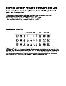
Figure 2 represents four different structures for Brain Tumor dataset. Structure A is the one introduced by G. F. Cooper. Structures B (β = 1.0, α = 1.0, r = 3), C(β = 1.0, α = 0.8, r = 2) and D(β = 2.1, α = 0.5, r = 3) are the ones generated by our approach.

4

Conclusions

We developed an approach for generating a Bayesian network structure from data based on notion of generalized entropy. The best parent-child relationships among attributes is obtained at values of β that are highly dependent on the data set, a fact that suggests that the GCE approach is preferable to using the Shannon entropy.

References Beinlich, I., H. Suermondt, R. Chavez, and G. F. Cooper (1989). The ALARM monitoring system: A case study with two probabilistic inference techniques for belief networks. Technical Report KSL-88-84, Stanford University, Knowledge System Laboratory. Blake, C., D. Newman, S. Hettich, and C. Merz (1998a). UCI repository of machine learning databases. A dataset from Ljubljana Oncology Institute provided by UCI, available at http://www.ics.uci.edu/ mlearn/MLRepository.html. Blake, C., D. Newman, S. Hettich, and C. Merz (1998b). UCI repository of machine learning databases. A dataset created by R.A. Fisher and donated by Michael Marshall, available at http://www.ics.uci.edu/ mlearn/MLRepository.html. Cooper, G. F. (1984). NESTOR: A computer-based medical diagnosis aid that integrates casual and probabilistic knowledge. Ph. D. thesis, Stanford University. Cooper, G. F. and E. Herskovits (1993). A Bayesian method for the induction of probabilistic networks from data. Technical Report KSL-91-02, Stanford University, Knowledge System Laboratory. RNTI - X -

Inference of Bayesian Networks

F IG . 2 – Brain Tumor Structures

Havrda, J. H. and F. Charvat (1967). Quantification methods of classification processes: Concepts of structural α entropy. Kybernetica 3, 30–35. Lam, W. and F. Bacchus (1994). Learning Bayesian belief networks: An approach based on the MDL principle. Computational Intelligence 10, 269–293. Rissanen, J. (1978). Modeling by shortest data description. Automatica 14, 456–471. Simovici, D. A. and S. Jaroszewicz (2002). An axiomatization of partition entropy. Transactions on Information Theory 48, 2138–2142. Simovici, D. A. and S. Jaroszewicz (2006). A new metric splitting criterion for decision trees. International Journal of Parallel, Emergent and Distributed Systems 21, 239–256. Suzuki, J. (1999). Learning Bayesian belief networks based on the MDL principle: An efficient algorithm using the branch and bound technique. IEICE Trans. Information and Systems, 356–367. Williams, M. and J. Williamson (2006). Combining argumentation and Bayesian nets for breast cancer prognosis. Journal of Logic, Language and Information 15, 155–178.

Résumé Nous proposons un nouvel algorithme pour extraire la structure d’un réseau Bayésien d’un ensemble de données. Notre approche est basée sur les entropies conditionnelles généralisées, une famille conditionnelle d’entropies qui étend l’entropie conditionnelle de Shannon.Nos résultats indiquent que, avec un choix approprié d’une entropie conditionnelle généralisée, nous obtenons des réseaux Bayésiens qui ont des scores supérieurs aux structures similaires obtenues par des méthodes classiques d’inférence. RNTI - X -