Structure-preserving properties of bilevel image compression

Human Vision and Electronic Imaging XIII, B. E. Rogowitz and T. N. Pappas, eds., Proc. SPIE Vol. 6806, (San Jose, CA), Jan. 28 - 31, 2008.

Structure-preserving properties of bilevel image compression Matthew G. Reyes,a Xiaonan Zhao,b David L. Neuhoff,a and Thrasyvoulos N. Pappasb a EECS

Departpment, University of Michigan, Ann Arbor, MI 48109; Department, Northwestern University, Evanston, IL 60208

b EECS

ABSTRACT We discuss a new approach for lossy compression of bilevel images based on Markov random fields (MRFs). The goal is to preserve key structural information about the image, and then reconstruct the smoothest image that is consistent with this information. The image is compressed by losslessly coding the pixels in a square grid of lines and adding bits when needed to preserve structural information. The decoder uses the MRF model to reconstruct the interior of each block bounded by the grid, based on the pixels on its boundary, plus the extra bits provided for certain blocks. The idea is that, as long as the key structural information is preserved, then the smooth contours of the block having highest probability with respect to the MRF provides acceptable reconstructions. We propose and consider objective criteria for both encoding and evaluating the quality and structure preserving properties of the coded bilevel images. These include mean-squared error, MRF energy (smoothness), and connected components (topology). We show that overall, for comparable mean-squared error, the new approach provides perceptually superior reconstructions than existing lossy compression techniques at lower encoding rates. Keywords: Binary images, object-based coding, structural similarity, JBIG, JBIG2

1. INTRODUCTION Compression of bilevel images is an important special case of image compression, both because some images are by their own nature bilevel (e.g., text, graphics, halftones, pen and ink sketches) and because they can be used to represent segmentation information for a variety of applications, including object-based compression (e.g., MPEG-41 and second generation image coding techniques2 ), object or region of interest specification, and foreground/background detection. As in any compression application, the goal is to encode the source using as few bits as possible, while retaining an accurate representation of the visual information present in the source. The lossless compression of bilevel images has received a lot of attention in the literature, primarily because of the facsimile standards. The Group 3 and 4 facsimile standards3 rely on efficient text compression algorithms, while the more recent JBIG standard3 provides a efficient lossless bilevel compression for a wide variety of image types that include text, graphs, binary objects of various shapes, and even some (periodic) halftoning techniques. However, the resulting bit rates are relatively high, which creates a need for lossy techniques that provide high fidelity approximations of the bilevel images without substantial perceptual losses. In particular, it is wellestablished in the object-based coding literature that coding of the object contours accounts for a significant percentage of the overall bit rate. The recently proposed JBIG2 standard4 aims to provide much higher compression ratios with almost no degradation in image quality. In JBIG2, the bilevel image is first divided into different region types (text, graphs, and halftones), and each region is encoded with an appropriate scheme. The first stage of the standard includes algorithms for encoding bilevel images of text and halftones, but cannot yet handle general bilevel images or object outlines. However, a lossy coder for bilevel images could consist of a lossy operation, such as morphological smoothing, followed by lossless JBIG. We will show that the proposed techniques outperform such schemes in the rate distortion sense. There is also a substantial literature on techniques for lossy compression of object contours (e.g., for MPEG-45, 6 ). The applicability of such techniques is limited, however, because they assume well-defined binary objects. Finally, Culik and Valenta have proposed an interesting lossy coding Further author information: (Send correspondence to T.N.P.) Email: mreyes,[email protected], [email protected], [email protected]

technique for bilevel images based on finite-state automata.7, 8 We will compare our new techniques to this method, which has a resemblance to fractal image coding. In this paper, we discuss a new method for lossy compression of bilevel images that is based on Markov random fields (MRFs).9 The goal is to find a specification that preserves the key structural information in the image, and then to reconstruct the smoothest image that is consistent with this specification. One such specification consists of the (original) image pixels in a square line grid, plus additional bits that may be needed to preserve structural information in the interior of the grid cells. The pixels on the grid are compressed with a lossless encoding technique (e.g., arithmetic or Huffman coding). We consider a fixed block size for the specification, but the proposed method can be easily extended to a quadtree approach that adjusts the block size to local image detail. The decoder uses a MRF-based model to reconstruct the interior of each block bounded by the grid, based on the pixels on its boundary, plus the extra bit(s) provided for some of the blocks. The idea is that, as long as the key structural information is preserved, then smooth contours in the block (having highest probability with respect to the MRF) provide acceptable reconstructions. We argue that the proposed scheme provides structurally lossless compression, in the sense that the key image structure is preserved, even though there are obvious differences (in a side-by-side comparison) between the original and reconstructed images. This is in contrast to perceptually lossless compression,10–12 whereby the original and reconstructed images are indistinguishable. It is interesting to compare this new approach to a more conventional one that would specify, i.e. losslessly encode, a grid of points rather than a grid of lines. That is, consider subsampling the image by a factor N in each dimension and then losslessly encoding these subsamples. While it might at first seem that specifying lines rather than points would be expensive in terms of bit rate, in fact, the high correlation between adjacent grid pixels substantially mitigates the increased number of pixels in the specification, while the line grid specification greatly enhances the ability of the decoder to make good reconstructions of the unspecified portions of the image. We propose and consider several objective criteria for both encoding and evaluating the quality and structure preserving properties of the coded bilevel images. These include mean-squared error, MRF energy (smoothness), and connected components (topology). We show that overall, for comparable mean-squared error, the new technique provides perceptually superior reconstructions than existing lossy compression techniques at lower encoding rates. In the remainder of this paper, Section 2 provides an overview of the bilevel encoding and decoding system including the MRF model. Section 3 examines different performance metrics, and Section 4 discusses results and conclusions.

2. LOSSY COMPRESSION OF BILEVEL IMAGES In this section, we review a lossy bilevel compression algorithm that was proposed in Ref. 9. The encoder uses a lossless scheme (arithmetic, Huffman) to encode a subset of the image pixels on a rectangular (square) grid, plus a number of additional bits that provide information about image structure in the interior of the grid cells. The decoder reconstructs the remaining pixels based on the available information, using a maximum a posteriori (MAP) formulation with respect to a Markov random field model of the image.

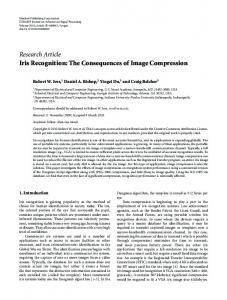
2.1 Specification The image specification consists of a subset of the pixels of the original bilevel image, typically on a rectangular grid. An 8 × 8 grid and the corresponding specification are shown in Fig. 1. A detail of the encoder specification is shown in Fig. 2. Other regular (e.g., hexagonal) or spatially adaptive (e.g., the grid size depends on local image detail) grids may be used. For the following discussion, we will assume that the grid consists of square blocks of a fixed size N . The value of N typically ranges from 2 to 16. We losslessly encode the pixels in an N × N square grid. More specifically, we encode the pixels in rows 1, N + 1, 2N + 1, . . ., and in columns 1, N + 1, 2N + 1, . . ., as well as the rightmost column and bottom row, if not already encoded. Note that the unencoded pixels form (N − 1) × (N − 1) square blocks separated from each other by the encoded grid. Figure 1 shows a portion of the pixels in an N = 8 grid.

(a)

(b)

(c)

Figure 1. (a) Original bilevel image. (b) 8 × 8 grid. (c) The corresponding image specification. The interior pixels of each block, which are not encoded, are shown in gray.

There are many potential ways to losslessly encode the pixels in the grid. For example, they might be arranged into a sequence for arithmetic or runlength coding. However, in this paper, as a simple demonstration of the potential of this method, we consider arithmetic coding in which each grid pixel is encoded based on the first-order conditional probability, given one previously encoded pixel that is vertically or horizontally adjacent. Not surprisingly, we have found that the bit rate of the encoding is very close to H(X2 |X1 ), the conditional entropy of one pixel given a horizontally or Figure 2. Detail showing the pixels of 9 blocks and vertically adjacent pixel. Clearly, higher-order conditioning their specification via the grid. has the potential to work even better. Another possibility would be to specify (i.e., losslessly encode) a grid of points rather than a grid of lines, equivalently, to subsample by N in each dimension. While it may seem that specifying lines rather than points is expensive in terms of bit rate, in fact, the high correlation between adjacent grid pixels substantially mitigates the increased number of pixels in the specification, while the line grid specification greatly enhances the ability of the decoder to make good reconstructions of the unspecified portions of the image. As we will see below, in addition to the grid specification, we may also encode one or more additional bits that provide information about the structure of the interior of the block. We now discuss the MRF model on which the MAP reconstruction of the interior of each grid block given the pixels on its boundary will be based.

2.2 Markov Random Field Model Recall that an MRF is specified by a graph G = (V, E) and a collection of clique potential functions Ψ c (x). Here V is a finite set of nodes – in our case the pixel locations of the image – and E is a set of pairs of nodes. The members of E are considered to be (undirected) edges of the graph. Moreover, E defines a neighborhood relation between nodes, in the sense that two nodes are neighbors if and only if they are connected by an edge. Here edges indicate direct interpixel dependencies. As clique c is a subset of nodes in V such that all pairs of nodes in c are neighbors, i.e. are connected by an edge. Let C denote the collection of all cliques in G. Now consider a bilevel image x that assigns a zero (white) or one (black) to each pixel location in V . For each c ∈ C, a clique potential function Ψc (x) assigns a value to x that depends only the pixel values of x in the locations specified by c. Now, for this MRF model, the probability of a specific bilevel image x is given by ( ) X 1 Ψc (x) (1) p(x) = exp − Z c∈C

(a)

(b)

(c)

Figure 4. (a) Block specification. (b) High probability reconstruction. (c) Low probability reconstruction.

where Z is a normalizing constant. A path in a graph is a sequence of vertices p 1 , · · · , pm such that {pi , pi+1 } ∈ E, i = 1, · · · , m − 1. By the Global Markov Property,13 if A, B, and C are subsets of nodes such that every path from a node in A to a node in B includes a node from C, then the random variables XA and XB are conditionally independent of each other given the values XC . With an MRF model, the probability of an image is a product of functions defined over the cliques in the graph, and the cliques C are determined by the edge set E. Therefore the edges in a graphical model influence what images and patterns are more probable under that model. We initially considered two different edge sets for our model. The first is the Ising or 4-point model of statistical physics, in which edges connect horizontally and vertically adjacent nodes. The second we refer to as the diagonal or 8-point model. Its edge set connects horizontally, vertically, and diagonally adjacent nodes. The nodes and edges for the two types of grids are shown in Fig. 3. The only cliques in the Ising model are singletons or pairs of adjacent horizontal or vertical nodes, whereas in the diagonal model the cliques are singletons, pairs of adjacent nodes, triplets of adjacent nodes forming a right triangle, and quadruples forming a square. For cliques consisting of a single pair of nodes, the potential function we choose assigns −β if the nodes have the same value, and assigns +β if they have different values. For cliques consisting of one, three or four nodes, the potential function always assigns 0. Under this model, homogeneous regions and continuous contours are favored, i.e., assigned higher probability, over noisy regions and discontinuous contours. The theory of Markov random fields14, 15 has been used extensively in image processing, especially in segmentation, texture analysis and synthesis, restoration, and other applications, including image compression.16 One of the attractive properties of MRFs is their ability to impose some degree of structural coherence (spatial continuity constraints) to an image or image region. While the use of MRFs in image compression is not new, the proposed approach is unique in using MRFs solely for image reconstruction in the decoder.

2.3 Decoding/Reconstruction

(a)

(b)

Figure 3. The nodes and edges between nodes of an 8 × 8 block (a) Ising model. (b) Diagonal model.

The decoder first reconstructs the pixels on the grid, which have been losslessly encoded. Then it finds a MAP estimate of the pixels in the interior of each block given the values on the grid, and any additional information about the interior pixels. From the Global Markov Property, the interior of a block can be reconstructed using only the pixels on the boundary of that block. Thus, the decoding of each block is independent of the decoding of all the other blocks in the image. As mentioned previously, based on an MRF model, the conditional (on the boundary specification) probability of a block decreases monotonically with the number of pairs of adjacent nodes in the block having different values, which we call dissimilar pairs. Therefore, a block has maximum probability given the boundary if and only if it has fewest dissimilar pairs. This is illustrated in Fig. 4 It should be obvious that the fewer the dissimilar pairs, the smoother the resulting reconstruction. There are several cases to consider, illustrated in Figs. 5 and 8. First, if the boundary consists entirely of 0’s (respectively 1’s), as in Fig. 5 (a), then it is easy to see that the MAP reconstruction is entirely 0’s (respectively 1’s).

(a)

(b)

(c)

(d)

Figure 5. (a) “Zero” run. (b) One 1-side run. (c) One 2-side run. (d) One 3-side run.

(a)

(b)

(c)

(d)

Figure 6. (a) Boundary specification. (b), (c), (d) Three equiprobable reconstructions, based on the Ising model.

(a)

(b)

(c)

(d)

Figure 7. (a) Boundary specification. (b), (c), (d) Three equiprobable reconstructions, based on the diagonal model.

Second, suppose the boundary contains one run of consecutive 1’s, and all other boundary pixels are 0. Denote the first and last pixels of the run by P1 and P2. If P1 and P2 are on the same side of the block, as in Fig. 5 (b), then it is easy to see that the MAP reconstruction fills the interior with all 1’s or all 0’s, depending on which is more prevalent on the boundary. If P1 and P2 are on different sides, as illustrated in Fig. 5 (c) and (d), then it is easy to show that a MAP reconstruction is determined by a path of pixels from P1 to P2 through the interior of the block. (A path is a sequence of distinct neighboring pixels.) The pixels on the path, and those between the path and the run of 1’s on the boundary, are reconstructed as 1; all others as 0. It can be shown that if the vertical distance between P1 and P2 exceeds the horizontal distance, then a path is optimal, i.e., it determines a MAP reconstruction, if and only if it is a shortest path from P1 to P2. In the Ising model, this equivalent to saying that on a MAP path from P1 to P2, each step must decrease the distance to P2. In the 8-point model, this means that a MAP path consists entirely of vertical and diagonal steps in the direction of P2. A similar rule applies when the horizontal distance exceeds the vertical distance. It is now evident that there are usually a number of MAP reconstructions. As we can see in Fig. 6, the MAP reconstructions in the Ising model exhibit a great deal of variability. As illustrated in Fig. 7, in the 8-point model, the diagonal edges enforce greater continuity in the contours of the MAP reconstructions, and moreover, the entire range of reconstructions is more acceptable than that of the Ising model. For that reason we adopt the diagonal model for our implementation, and select one of the MAP reconstructions at random. Third, the boundary contains two runs of 1’s separated by zeros, as illustrated in Fig. 8. Then it can be shown that the MAP reconstruction is obtained by selecting two paths, each connecting a pair of run endpoints,

(a)

(b)

(c)

(d)

(e)

Figure 8. (a,d) Boundary specifications. (b,c) and (e,f) Structurally different reconstructions.

(f)

Figure 9. An example of a specification and the corresponding reconstruction. For illustrative purposes, in the middle and right figures, each block has been separated from its neighbors.

and filling in the remaining pixels in the natural way. There are two possible ways of pairing endpoints, as illustrated in the figure. For any given pairing, a path is optimal if and only if it satisfies the condition in the second case above. Each way of pairing run endpoints can be considered and the one creating a block with fewest dissimilar pairs is selected. We will refer to the encoder that uses this rule as the basic encoder. Note, however, that the two reconstructions are structurally different. Thus, it is worth investing an additional bit to specify which of the two reconstructions “best represents” the original image. We will refer to the encoder that includes the additional information as the decision-bit encoder. As we will discuss below, the selection of the appropriate reconstruction is not trivial, and requires an objective criterion, which should preferably preserve the structural information in the image. Finally, when the boundary contains three or more runs of 1s, true MAP reconstruction becomes more complex, especially when N is not small. However, since this does not happen often, we simply use the ad hoc approach of choosing the two longest runs of 1s on the boundary, and reconstructing the interior as described in the previous paragraph, as if all other pixels on the boundary were 0. The overall decoding process is illustrated in Fig. 9. In the above discussion, we have considered a fixed block size for the specification. However, the approach can be easily extended to a quadtree approach that adjusts the block size to local image detail. For that, as we will see in the next section, we will need an error metric that accurately reflects whether the reconstruction preserves the structural information in the image.

2.4 Criteria for Encoding with a Decision Bit As we saw above, when a block has two runs of 0’s and 1’s on its boundary, there are two ways of pairing endpoints of runs that produce structurally different reconstructions. As we will see in Section 4, in the basic encoder, the MAP reconstruction sometimes chooses an unfortunate pair of paths. For this reason, in the decision-bit encoder, we try both ways of pairing run end points, and use one bit to indicate the one which creates the reconstruction that best matches the original. A similar strategy, with additional bits, can be used when there are three or more runs on the boundary. We will demonstrate that this results in a significant increase in reconstruction quality for a small increase in bit rate. We now consider different criteria for finding the reconstruction that “best” matches the original image. Our goal is to preserve the structure of the original image. The simplest criterion is to find the number of pixels that are changed by the encoding/decoding process. For bilevel images, this is equivalent to mean squared error (MSE). An alternative is to choose the endpoint pairings that result in the same number of black connected components within the reconstructed block as in the original. Although this preserves topological structure, it is sensitive to errors, and can lead to perceptually significant distortions. An example is illustrated in Figure 10. Note that a change of just one pixel in the original image changes the number of connected components in the block, resulting in two different ways of pairing run endpoints, and consequently, structurally different reconstructions. On the other hand, the addition of the pixel has very little effect on the MSE. Thus, we see that the MSE criterion is quite robust and yields perceptually more meaningful results.

A

(a)

B

(b)

MSE-A=4 MSE-B=5

(c)

MSE-A=18 MSE-B=17

Figure 10. (a) Original blocks. (b) Boundary specification. (c) Two structurally different reconstructions.

3. PERFORMANCE METRICS The goal of image compression in general, and lossy bilevel image compression in particular, is to provide a balance between bit rate and reconstructed image quality. In this section, we examine different criteria for evaluating the performance of a bilevel coder. As mentioned in the introduction, lossless compression does not provide satisfactory results in terms of bit rate, so there is a need to allow some distortions in order to obtain higher compression. We are seeking high fidelity approximations without substantial perceptual losses. If we look at the grayscale image compression literature, the goal might be to obtain perceptually lossless compression.10–12 That is, an observer should not be able to distinguish the original and reconstructed images in a side-by-side comparison. There are several difficulties, however, with this type of criterion. First, since the images are bilevel, it is fairly easy for the human eye to spot changes, sometimes of even a single pixel. To avoid such problems in the compression of halftone images,11 it was found necessary to add micro-dither to images halftoned with a classical screening technique. Here, however, it does not make sense to add microdither. Another difficulty is that the perceptual quality metrics that have been developed for grayscale compression 10–12 cannot be used to evaluate bilevel image quality. An alternative is to give up on perceptual transparency and to consider structurally lossless compression. By this we mean that, even though there may be noticeable differences in a side-by-side comparison, the reconstructed image conveys the same (structural) information as the original, and if viewed separately, it may not even be possible to decide which of the two images is the original one. In this paper, we argue that the new compression scheme can produce structurally lossless compression. However, it is difficult to derive objective criteria that reflect the resulting quality. In the following, we propose and analyze a number of objective criteria for evaluating the performance and structure preserving properties of coded bilevel images including the new approach. A traditional approach to measure image quality is by the fraction of pixels changed by encoding/decoding. We refer to this as the error rate. For bilevel images, this is equivalent to MSE. However, as we will see in the next section, two images with similar MSE, can have quite different appearance. By construction, the new methods preserve the structural information in the bilevel image. This can be attributed to two key elements of the coder. The first is the grid specification, and the second is the additional bits describing the structure of the interior. Of course, as we saw in the previous section, another key element is the metric that is used to determine which is the structurally most relevant reconstruction. Another distinguishing characteristic of a bilevel image reconstruction is the smoothness of the edges and how it compares to the smoothness of the original image. One approach to evaluating the smoothness of an image is via the formalism of MRFs that we introduced in Section 2. We can compare the MRF energy of the original and reconstructed image, either globally, or locally. According to the MRF model, the probability of the bilevel image, or image segment, x is given by (1). In order to avoid problems with boundary conditions, we will consider the conditional probability of a W × W block of pixels, given the pixels on the block boundary outside the block (assuming the diagonal MRF model). We can then compare the smoothness of the original and reconstructed images at a given pixel s, by comparing the probabilities of the W × W blocks, which from now on we call windows, centered at s. In the limiting case of a window consisting of a single pixel, we obtain the conditional probability of the pixel, given its eight neighbors. The following metric will then reflect the similarity in smoothness between the original window x and reconstructed window x ˆ. p x) 2 p(x)p(ˆ (2) SmSIM = p(x) + p(ˆ x)

(a)

(b)

(c)

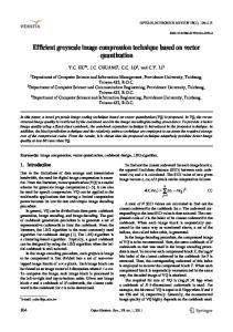
Figure 11. (a) Portion of an original image. (b) Decision-bit encoder. (c) Culik-Valenta.

Note that the calculation of the metric involves only ratios of the probabilities, and thus, does not require the normalizing constant (Z), which is hard to compute. The metric value ranges from 0 (when p(x) = 0 or p(ˆ x) = 0) to 1 (when p(x) = p(ˆ x)). This metric can be calculated by sliding the window over each pixel of the image. The resulting error map can then be averaged over the entire image to obtain the overall image smoothness. However, smoothness alone is not enough; the image must also be close to the original image. For that we can include a separate term. In order to present a formulation that includes this aspect of quality and is consistent with the MRF formulation, we can add singleton cliques with potential functions that assign −α (which corresponds to higher probability) when the pixels of the reconstructed image agree with the corresponding pixels in the original, and assign +α when they don’t. For the original image all the pixels are by default correct, so they are all assigned −α. Another formulation with identical results is to consider the two images as two consecutive frames of a sequence and to introduce cliques between the frames. In measuring the relative MRF energies, it is important to consider the horizontal/vertical transitions separately from the diagonal ones, because, as shown in Fig. 11, some techniques (e.g., Culik-Valenta) may introduce blocky artifacts, with more transitions in the horizontal and vertical directions than in the diagonal ones, while our techniques produce smoother edges with more equal distribution of transitions. Thus, we can consider separate MRF models, each with one type of clique, and then combine them multiplicatively, as is done in structural similarity metrics:17 SmSIM = SmSIMα ∗ SmSIMh ∗ SmSIMv ∗ SmSIMd ∗ SmSIMd0 (3) where the five terms correspond to the single, horizontal, vertical, diagonal, and anti-diagonal cliques. Finally, before combining the terms in (3), we apply Gaussian smoothing to each error map. We experimented with all of the above MRF-based metrics, and found that, for reasonable values of the parameters (β and α), they predict the relative performance of the different algorithms. However, the difference is typically in the second or third most significant digit of the metric value. On the other hand, the metrics scale down appropriately when two completely different images are compared, or when a random or halftone image is compared to the segmentation map. In the spirit of MRF energy, a simple indicator of the smoothness of the reconstructed image relative to the original, is the overall number of horizontal, vertical, and diagonal black/white transitions in the reconstructed image, expressed as a percentage of the corresponding transitions in the original image. As we will see in Section 4, the number of transitions in each of the four directions is a good indicator of smoothness and blockiness.

4. EXPERIMENTAL RESULTS In our experiments we used two sets of bilevel images obtained by segmentation of two original grayscale images. For the segmentation we used the adaptive clustering algorithm of Ref. 18. By controlling the parameters of the algorithm, we could generate bilevel images with different degrees of smoothness. Three of the images of each set are shown in Fig. 12. All images are 512 × 512. However, for simplicity, we cropped each image to a size that is a multiple of the size of the grid that we used for encoding. In addition to our new techniques, 9 we tested the lossy bilevel coding scheme of Culik and Valenta,7, 8 as well as a lossy coding scheme that consists of a morphological (median-type) smoothing filter followed by lossless JBIG compression. Figure 15 shows error rate vs. bit rate for each test image and encoding method. For our methods the different points in each curve were obtained by choosing block sizes 16, 14, 12, 10, 8, 6, 4, 2, 1, which have decreasing error

(A2)

(A3)

(A4)

(B2)

(B3)

(B5)

Figure 12. Test images in (left to right) rough to smooth order.

rate and increasing bit rate. For the Culik-Valenta method, the points were obtained by varying their quality factor. For the smoothing plus JBIG the points were obtained by varying the window size of a morphological filter. Each plot also includes the rate of lossless coding with our method (N = 1) and with JBIG. We see from these plots that the decision-bit MRF method is significantly better than both the basic MRF method and the Culik-Valenta method, with larger improvements at lower rates. We also see that it is much better than the JBIG smoothing method, except at very low error rates. For instance, at zero error-rate, JBIG is better than our N = 1 lossless coder, which is to be expected, since as a lossless coder it is overly simplistic. Figure 13 shows the results of encoding/decoding the image “A2” with, the basic method with grid size N = 8, the decision-bit method with N = 8, and the method of Culik-Valenta. The corresponding points in the plot of Fig. 15 are highlighted with circles. Note that the bit rates for the basic and decision-bit methods are about the same, but the latter has lower error. The bit rate for the Culik-Valenta reconstruction is higher, while the error rate is similar to that of the decision-bit method. We observe that the basic method has turned some thin lines into dotted lines (e.g., the black lines in the shirt collar and the white lines lines in the hair), while the eyes have lost detail.. This is due to the MAP reconstruction of blocks whose boundaries have two or more runs of 1’s. The reconstruction in the decision-bit method fixes this problem. By preserving the structural integrity of the image, the decision-bit method produces larger gains of perceptual quality than what one might expect from the error rate improvements shown in Fig. 15. To some extent, the Culik-Valenta method also seems to preserve the structural integrity of the image, but tends to produce reconstructions with rough contours and unnaturally sharp angles, which are quite noticeable. Figure 14 shows demonstrates the performance of the three approaches when they are applied to image “B3.”

(a)

(b)

(c)

Figure 13. Reproduction of image A2 after coding/decoding with (a) the basic method (N = 8), (b) the decision-bit method (N = 8), and (c) the Culik-Valenta method at a similar error rate.

(a)

(b)

(c)

Figure 14. Reproduction of image B3 after coding/decoding with (a) the basic method (N = 8), (b) the decision-bit method (N = 8), and (c) the Culik-Valenta method at a similar error rate.

Image A2 B3

Basic Encoder 0.9446 0.9315

Decision-Bit Encoder 0.9548 0.9428

Culik-Valenta 0.9513 0.9368

Table 1. Percent error rate, and percentage of directional transitions in reconstructed image A2.

Again, the corresponding points are highlighted with circles in the plot of Fig. 15. The observations are similar in this example, with the decision-bit method providing the best overall performance. A comparison of Figures 13(b) and (c) demonstrates that the error rate is not a good indicator of image quality, as the two images have the same error rate but significant differences in perceptual quality. Table 1 shows the values of the metric of (3), calculated using a 3 × 3 window and Gaussian smoothing, β = 0.5, and α = 1.0. Note that this metric predicts the relative performance of the different three algorithms. However, the difference is typically in the second or third most significant digit of the metric value. We now turn to the simple indicator of relative smoothness that we also discussed in Section 3, which measures the overall number of horizontal, vertical, and diagonal black/white transitions in the reconstructed image as a percentage of the corresponding transitions in the original image. The results are shown in Table 2. Note that the decision-bit encoder reduces the transitions in all directions resulting in a smoother image, while the Culik-Valenta algorithm tends to increase the diagonal and anti-diagonal transitions. This is a good indicator of blockiness. The performance of the basic coder is not competitive with the others in this case, but typically, it

0.1

0.06

error rate

error rate

0.08

0.04

(A2)

0.02 0 0

0.05

0.1 0.15 bit rate

0.1

0.04

(A3)

0.02 0.05

0.1 bit rate

0.1

0.2

0.04

(A4)

0.02 0 0

0.05

0.1 bit rate

0.15

0.05

0.1 0.15 bit rate

0.2

MRF Basic MRF Decision JBIG Culik

0.05

(B3)

0.05

0.1 bit rate

0.15

error rate

0.06

(B2)

0.1

0 0

MRF Basic MRF Decision JBIG Culik

0.08 error rate

0.15

0.05

0.15

error rate

error rate

0.06

MRF Basic MRF Decision JBIG Culik

0.1

0 0

0.2

MRF Basic MRF Decision JBIG Culik

0.08

0 0

0.15

MRF Basic MRF Decision JBIG Culik

0.2

MRF Basic MRF Decision JBIG Culik

0.1

0.05

0 0

0.15

(B5)

0.05

0.1 bit rate

0.15

Figure 15. Error rate versus bit rate for the various encoding methods and three versions of the two test images. The decoded images corresponding to the circled points are shown in Figs. 13 and 14.

Basic Encoder Decision-bit Encoder Culik-Valenta

error rate 0.048 0.023 0.023

horizontal 81.1 92.1 97.4

vertical 84.2 88.3 94.8

diagonal 71.5 92.4 104.4

anti-diagonal 113.3 92.1 103.7

Table 2. Percent error rate, and percentage of directional transitions in reconstructed image A2, compared to the original.

tends to increase smoothness. In summary, we have observed that the decision-bit MRF method generally produces reconstructed images that preserve structure and overall quality at favorable bit rates.

REFERENCES [1] ISO/IEC 14496, “Information technology – generic coding of audio-visual objects,” July 1999. [2] M. Kunt, A. Ikonomopoulos, and M. Kocher, “Second-generation image-coding techniques,” Proc. IEEE 73, pp. 549–574, Apr. 1985. [3] K. Sayood, Introduction to Data Compression, ch. 10. Morgan Kaufmann, 2006. [4] P. G. Howard, F. Kossentini, B. Martins, S. Forchhammer, and W. J. Rucklidge, “The emerging JBIG2 standard,” IEEE Trans. Circuits Syst. Video Technol. 8, pp. 838–848, Nov. 1998. [5] A. K. Katsaggelos, L. P. Kondi, F. W. Meier, J. Ostermann, and G. M. Schuster, “MPEG-4 and ratedistortion-based shape-coding techniques,” Proc. IEEE 86, pp. 1126–1154, June 1998. special issue on Multimedia Signal Processing. [6] A. Vetro, Y. Wang, and H. Sun, “Rate-distortion modeling for multiscale binary shape coding based on Markov random fields,” IEEE Trans. Image Process. 12, pp. 356–364, Mar. 2003. [7] K. C. II and V. Valenta, “Finite automata based compression of bi-level and simple color images,” in Proc. IEEE Data Compression Conf., (Snowbird, Utah), 1996. [8] K. C. II and V. Valenta, “Finite automata based compression of bi-level and simple color images,” Computer & Graphics 21(1), pp. 61–68, 1997. [9] M. G. Reyes, X. Zhao, D. L. Neuhoff, and T. N. Pappas, “Lossy compression of bilevel images based on Markov random fields,” in Proc. Int. Conf. Image Processing (ICIP-07), 2, pp. II–373–II–376, (San Antonio, TX), Sept. 2007. [10] R. J. Safranek and J. D. Johnston, “A perceptually tuned sub-band image coder with image dependent quantization and post-quantization data compression,” in Proc. ICASSP-89, 3, pp. 1945–1948, (Glasgow, Scotland), May 1989. [11] D. L. Neuhoff and T. N. Pappas, “Perceptual coding of images for halftone display,” IEEE Trans. Image Processing 3, pp. 341–354, July 1994. [12] T. N. Pappas, R. J. Safranek, and J. Chen, “Perceptual criteria for image quality evaluation,” in Handbook of Image and Video Processing, A. C. Bovik, ed., pp. 939–959, Academic Press, second ed., 2005. [13] S. L. Lauritzen, Graphical Models, Oxford Press, 1996. [14] J. Besag, “Spatial interaction and the statistical analysis of lattice systems,” J. Royal Statist. Soc. B 26(2), pp. 192–236, 1974. [15] J. Besag, “On the statistical analysis of dirty pictures,” J. Royal Statist. Soc. B 48(3), pp. 259–302, 1986. [16] G. Gelli, G. Poggi, and R. P. Ragozini, “Multispectral-image compression based on tree-structured Markov random filed segmentation and transform coding,” in Proc. IEEE Geoscience and Remote Sensing Symp. (IGARSS), 2, pp. 1167–1170, 1999. [17] Z. Wang, A. C. Bovik, H. R. Sheikh, and E. P. Simoncelli, “Image quality assessment: From error visibility to structural similarity,” IEEE Trans. Image Process. 13, pp. 600–612, Apr. 2004. [18] T. N. Pappas, “An adaptive clustering algorithm for image segmentation,” IEEE Trans. Signal Process. SP40, pp. 901–914, Apr. 1992.