STRUCTURE RELATIONS IN SPECIAL A ... - Semantic Scholar

Journal of Mathematical Sciences, Vol. 152, No. 3, 2008

STRUCTURE RELATIONS IN SPECIAL A∞ -BIALGEBRAS R. Umble

UDC 515.142.32

Abstract. We compute the structure relations in special A∞ -bialgebras whose operations are limited to those defining the underlying A∞ -(co)algebra substructure. Such bialgebras appear as the homology of certain loop spaces. Whereas structure relations in general A∞ -bialgebras depend upon the combinatorics of permutahedra, only Stasheff’s associahedra are required here.

CONTENTS 1. 2. 3. 4. 5.

Introduction . . . . . . Matrix Considerations Cup Products . . . . . Special A∞ -Bialgebras Structure Relations . . References . . . . . . .

. . . . . .

. . . . . .

. . . . . .

. . . . . .

. . . . . .

. . . . . .

. . . . . .

. . . . . .

. . . . . .

1.

. . . . . .

. . . . . .

. . . . . .

. . . . . .

. . . . . .

. . . . . .

. . . . . .

. . . . . .

. . . . . .

. . . . . .

. . . . . .

. . . . . .

. . . . . .

. . . . . .

. . . . . .

. . . . . .

. . . . . .

. . . . . .

. . . . . .

. . . . . .

. . . . . .

. . . . . .

. . . . . .

. . . . . .

. . . . . .

. . . . . .

. . . . . .

. . . . . .

. . . . . .

. . . . . .

. . . . . .

. 443 . 444 . 446 . 447 . 449 . 450

Introduction

A general A∞ -bialgebra is a DG-module (H, d) equipped with a family of structurally compatible operations ωj,i : H ⊗i → H ⊗j , where i, j ≥ 1 and i + j ≥ 3 (see [6]). In special A∞ -bialgebras, ωj,i = 0 for i, j ≥ 2 and the remaining operations mi = ω1,i and Δj = ωj,1 define the underlying A∞ -(co)algebra substructure. Thus, special A∞ -bialgebras have the form (H, d, mi , Δj )i,j≥2 subject to the appropriate structure relations involving d, mi , and Δj . These relations are much easier to describe than those in the general case, which require the S-U diagonal ΔP on permutahedra. Instead, the S-U diagonal ΔK on Stasheff’s associahedra K = Kn is required here (see [5]). A∞ -bialgebras are fundamentally important structures in algebra and topology. In general, the homology of every A∞ -bialgebra inherits an A∞ -bialgebra structure [7]; in particular, this holds for the integral homology of a loop space. In fact, over a field, the A∞ -bialgebra structure on the homology of a loop space specializes to the A∞ -(co)algebra structures observed by Gugenheim [2] and Kadeishvili [3]. The main result of this paper is the following simple formulation of the structure relations in special A∞ -bialgebras that do not involve d. Let T H denote the tensor module of H and let en−2 denote the top-dimensional face of Kn . There is a “fraction product” on M = End(T H) (denoted here by “•”) and certain cellular cochains ξ, ζ ∈ C ∗ (K; M ) such that for every i, j ≥ 2, Δj • mi = ξ j (ei−2 ) • ζ i (ej−2 ), where the exponents indicate certain ΔK -cup powers. Acknowledgment. I must acknowledge the fact that many of the ideas in this paper germinated during conversations with Samson Saneblidze, whose openness and encouragement led to this paper. For this, I express sincere thanks. This research was partially supported by a Millersville University faculty research grant. Translated from Sovremennaya Matematika i Ee Prilozheniya (Contemporary Mathematics and Its Applications), Vol. 43, Topology and Its Applications, 2006. c 2008 Springer Science+Business Media, Inc. 1072–3374/08/1523–0443 

443

@•

@•

6

•

@

2,4 A ∈ M1,3 ↔

@B•

KAA A A

↔

@B•

•

@

•

2

A

•

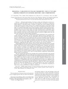
2 4 Fig. 1. Graphical representations of a typical monomial.

2.

Matrix Considerations

We begin with a brief review of the algebraic machinery we need; for a detailed exposition, see [6]. Let M = m,n≥1 Mn,m be a bigraded module over a commutative ring R with identity 1R and consider the module T T M of tensors on T M . Given matrices X = [xij ] and Y = [yij ] ∈ Nq×p , p, q ≥ 1, consider the submodule     MY,X = My11 ,x11 ⊗ · · · ⊗ My1p ,x1p ⊗ · · · ⊗ Myq1 ,xq1 ⊗ · · · ⊗ Myqp ,xqp ⊂ (M ⊗p )⊗q ⊂ T T M. Represent a monomial A = (θy11 ,x11 ⊗ · · · ⊗ θy1p ,x1p ) ⊗ · · · ⊗ (θyq1 ,xq1 ⊗ · · · ⊗ θyqp ,xqp ) ∈ MY,X as a (q × p)matrix [A] = [aij ] with aij = θyij ,xij . Then A is the q-fold tensor product of the rows of [A] considered as elements of M ⊗p ; we refer to A as a q × p monomial and often write A instead of [A]. The matrix submodule of T T M is the sum   M= MY,X = (M ⊗p )⊗q . X,Y ∈Nq×p p,q≥1

p,q≥1

Given x × y =(x1 , . . . , xp ) × (y1 , . . . , yq ) ∈ Np × Nq , we set X = [xij = xj ]1≤i≤q and Y = [yij = yi ]1≤j≤p and denote Myx = MY,X . The bisequence submodule of T T M is  Myx M= x×y∈Np ×Nq p,q≥1

and the (q × p)-monomial A ∈ M has the form ⎡ θy1 ,x1 ⎢ .. A=⎣ . θyq ,x1

··· ···

⎤ θy1 ,xp .. ⎥ . . ⎦ θyq ,xp

We represent A = [θyj ,xi ] ∈ Myx graphically in two ways: (1) as a matrix of “double corollas,” where θyj ,xi is pictured as two corollas joined at the root-one opening downward with xi leaves and the other opening upward with yj leaves and (2) as an arrow in the positive integer lattice N2 from (|x|, q) to (p, |y|), where (see Fig. 1). |u| = u1 + · · · + uk  Each pairing γ : r,s≥1 M ⊗r ⊗ M ⊗s → M induces an upsilon product Υ : M ⊗ M → M supported on “block transverse pairs,” which we now describe. Definition 1. A monomial pair Aq×s ⊗ B t×p = [θyk ,vk ] ⊗ [ηuij ,xij ] ∈ M ⊗ M is a 444

(i) transverse pair (TP) if s = t = 1, u1,j = q, and vk,1 = p for all j, k, i.e., setting xj = x1,j and yk = yk,1 gives ⎤ ⎡ θy1 ,p

⎥ ⎢ A ⊗ B = ⎣ ... ⎦ ⊗ ηq,x1 · · · ηq,xp ∈ Myp ⊗ Mqx ; θyq ,p  ] (ii) block transverse pair (BTP) if there exist (t × s)-block decompositions A = [Ak  ] and B = [Bij    such that Ai ⊗ Bi is a TP for all i, .  ) in a general BTP may vary in Unlike the blocks in a standard block matrix, the blocks Ai (or Bi y length within a given row (or column). However, when A ⊗ B ∈ Mv ⊗ Mux is a BTP with u = (q1 , . . . qt ),  ∈ Myi ⊗ Mqi so that for a fixed v = (p1 , . . . , ps ), x = (x1 , . . . , xs ), and y = (y1 , . . . , yt ), the TP Ai ⊗ Bi p x   i (or ) the blocks Ai (or Bi ) have a constant length qi (or p ); furthermore, A ⊗ B is a BTP if and only if y ∈ N|u| and x ∈ N|v| if and only if the initial point of the arrow A coincides with the terminal point of the arrow B. Note that BTP block decomposition is unique. 1,5,4,3 3,1 ⊗ M1,2,3 is a 2 × 2 BTP per the block Example 1. A pairing of monomials A4×2 ⊗ B 2×3 ∈ M2,1 decompositions





Given a pairing γ =

 x×y



θ1,2

θ1,1

θ5,2

θ5,1

θ4,2

θ4,1

θ3,2

θ3,1





η3,1

η3,2

η3,3

η1,2

η1,3

and

. η1,1 



|y|

γxy : Myp ⊗ Mqx → M|x| , extend γ to an upsilon product Υ : M ⊗ M → M via  Υ(A ⊗ B)i =

 ) if A ⊗ B is a BTP γ(Ai ⊗ Bi

0

(2.1)

otherwise.

 ∈ Myi ⊗ Mqi to a (t × s)-monomial Then Υ sends a BTP Aq×s ⊗ B t×p ∈ Myv ⊗ Mux with Ai ⊗ Bi p x |y1 |,...,|yt | in M|x1 |,...,|xs | . We denote A · B = Υ(A ⊗ B); if [θj ] ⊗ [ηi ] is a TP, we denote γ(θ1 , . . . , θq ; η1 , . . . , ηp ) = (θ1 ⊗ · · · ⊗ θq ) · (η1 ⊗ · · · ⊗ ηp ). As an arrow, A · B runs from the initial point of B to the terminal point of A. Note that M · M ⊆ M, so that Υ is restricted to an upsilon product on M. 1,5,4,3 3,1 ⊗ M1,2,3 produces a 2 × 2 Example 2. Continuing Example 1, the action of Υ on A4×2 ⊗ B 2×3 ∈ M2,1 10,3 monomial in M3,3 :





θ1,2 θ5,2





θ1,1 θ5,1

θ4,2

θ4,1

θ3,2

θ3,1



·



γ(θ1,2 , θ5,2 , θ4,2 ; η3,1 , η3,2 ) γ(θ1,1 , θ5,1 , θ4,1 ; η3,3 )

η3,1 η3,2 η3,3 = 

η1,1 η1,2 η1,3






γ(θ3,2 ; η1,1 , η1,2 )

γ(θ3,1 ; η1,3 )

. 



445

•

@

•

@

•

•

@

@•

@•

=

• @ @ @

@

@ @•

•

@

•

@

@

@ @

@

@ @•

Fig. 2. The γ-product as a nonplanar graph. In the target, (|x1 |, |x2 |) = (1 + 2, 3) since (p1 , p2 ) = (2, 1) and (|y1 |, |y2 |) = (1 + 5 + 4, 3) since (q1 , q2 ) = (3, 1). As an arrow, A · B initializes at (6, 2) and terminates at (2, 13). The applications below relate to the following special case: let H be a graded module over a commutative ring with unity and consider M = End(T H) as a bigraded module via Mn,m = Hom(H ⊗m , H ⊗n ). Then a q × p monomial A ∈ Myx admits a representation as an operator on N2 via (H ⊗|x| )⊗q ≈ (H ⊗x1 ⊗ · · · ⊗ H ⊗xp )⊗q −→ (H ⊗y1 )⊗p ⊗ · · · ⊗ (H ⊗yq )⊗p A

σy1 ,p ⊗···⊗σyq ,p

−→

σy1 ,p ⊗···⊗σyq ,p

−→

(H ⊗p )⊗y1 ⊗ · · · ⊗ (H ⊗p )⊗yq ≈ (H ⊗p )⊗|y| , ≈

where (s, t) ∈ N2 is identified with (H ⊗s )⊗t and σs,t : (H ⊗s )⊗t → (H ⊗t )⊗s is the canonical permutation of tensor factors     σq,p : (a11 · · · aq1 ) · · · (a1p · · · aqp ) → (a11 · · · a1p ) · · · (aq1 · · · aqp ) . The canonical structure mapping ∗  ιp ⊗ιq ◦ |y| qp id ⊗σq,p pq ⊗ M −→ M|y| γ= γxy : Myp ⊗ Mqx −→ M|y| pq pq ⊗ M|x| −→ M|x| , |x|

(2.2)

∗ is induced by σ where ιp and ιq are the canonical isomorphisms and σq,p q,p (see [1, 4]), induces a canonical associative Υ product on M whose action on matrices of double corollas typically produces a matrix of nonplanar graphs (see Fig. 2). In this setting, γ agrees with the composition product on the universal preCROC [8].

3.

Cup Products

The two pairs of dual cup products defined in this section play an important role in the theory of structure relations. Let (H, dt) be a DG-module over a commutative ring with unity. For every i, j ≥ 2, choose operations mi : H ⊗i → H and Δj : H → H ⊗j considered as elements of M =End(T H). Recall Kn and provide that planar rooted trees (PRTs) parameterize the faces of Stasheff’s associahedra K = n≥2

module generators for cellular chains C∗ (K) [4]. Whereas top-dimensional faces correspond to corollas, lower-dimensional faces correspond to more general PRTs. Now, given a face a ⊆ K, consider the class of all planar rooted trees with levels (PLTs) representing a and choose a representative with exactly one node in each level. In this way, we obtain a particularly nice set of module generators for C∗ (K), denoted by K. Note that the elements of a class of PLTs represent the same function obtained by the composition in various ways. The results obtained here are independent of the choice since they depend only on the function. 446

Let G be a DGA concentrated in degree zero and consider the cellular cochains on K with coefficients in G: C p (K; G) = Hom−p (Cp (K); G). A diagonal Δ on C∗ (K) induces a cup product  on C ∗ (K; G) via f  g = ·(f ⊗ g)Δ, where “·” denotes the multiplication in G. The bisequence submodule M, which serves as our coefficient module, is canonically endowed with dual ˇ associative wedge and Cech cross products defined on a monomial pair A ⊗ B ∈ Myv ⊗ Mux as follows:   A ⊗ B if v = x, ∧ ∨ A ⊗ B if u = y, and A × B = A×B = 0 otherwise. 0 otherwise, ∧

∨

∧

∨

∧

∨

and Myv × Myx ⊆ Myv,x . Thus, Denote M = (M,×) and M = (M, ×) and note that Myx × Mux ⊆ My,u x nonzero cross-products concatenate matrices: A ∧ ∨ and A × B = [AB]. A×B = B ∧

∨

As arrows, A × B runs from vertical x = |x| to vertical x = p, whereas A × B runs from horizontal y = q ∧

is an arrow from (a, n) to (1, nb) and to horizontal y = |y|. In particular, if A ∈ Mba , then A×n ∈ Mb···b a ∨

A×n ∈ Mba···a is an arrow from (na, 1) to (n, b). These cross-products, together with the S-U diagonal ∧ ∨ ˇ cup products ∧ and ∨ in C ∗ (K; M) and C ∗ (K; M), respectively. ΔK [5], induce wedge and Cech ∧

∨

The modules C ∗ (K; M) and C ∗ (K; M) are equipped with second cup products ∧ and ∨ arising from the Υ-product on M together with the “leaf coproduct” Δ : C∗ (K) → C∗ (K) ⊗ C∗ (K), which we now define. Let T = T 1 ∈ K be a k-level PLT. Truncate T immediately below the first (top) level, trimming off a single corolla with n1 leaves and r1 − 1 stalks. Enumerating from left to right, let i1 be the position of the corolla. The (first) leaf sequence of T is the r1 -tuple xi1 (n1 ) = (1 · · · n1 · · · 1) with n1 in position i1 and 1 elsewhere. Denote the truncated tree by T 2 ; inductively, the jth leaf sequence of T is the leaf sequence of T j . The induction terminates when j = k; in this case, ik = rk = 1 and xik (nk ) = nk . The descent sequence of T is the k-tuple (xi1 (n1 ), . . . , xik (nk )). Definition 2. Let T ∈ K and identify T with its descent sequence n =(n1 , . . . , nk ). The leaf coproduct of T is given by ⎧  ⎨ (n1 , . . . , |ni |) ⊗ (ni , ni+1 , . . . , nk ), k > 1 Δ (T ) = 2≤i≤k ⎩ 0, k = 1. ∧

∨

Define the leaf cup products ∧ and ∨ on C ∗ (K; M) and C ∗ (K; M) as follows: f ∧ g = ·(f ⊗ g)τ Δ and f ∨ g = ·(f ⊗ g)Δ , where τ interchanges tensor factors and · denotes the Υ-product. Note that all cup products defined in this section are nonassociative and noncommutative. Unless otherwise explicitly indicated, iterated cup products are parenthesized on the extreme left, e.g., f ∨g ∨h = (f ∨ g) ∨ h. 4.

Special A∞ -Bialgebras

Structural compatibility of d, mi , and Δj is expressed in terms of the (restricted) biderivative dω and the “fraction product” • by the equation dω • dω = 0. We begin with a construction of the biderivative 447

ϕ

•


A@
A@

= m5 ,

ψ

@A
@ A•


= Δ5 .

Fig. 3. The actions of ϕ and ψ. ∧

∨

in our restricted setting. Let ϕ ∈ C ∗ (K; M) and ψ ∈ C ∗ (K; M) be the cochains with top-dimensional support such that ϕ(ei−2 ) = mi and ψ(ej−2 ) = Δj . We consider ϕ and ψ as acting on up-rooted and down-rooted trees, respectively (see Fig. 3). ∧

Let T c H denote the tensor coalgebra of H. The coderivation cochain of ϕ is the cochain ϕc ∈ C ∗ (K; M) that extends ϕ to cells of K in codim 1 so that  ϕc (e) ∈ Coder(T c H) codim e=0,1

 is the co-free linear coextension of ϕ(K) = i≥2 ϕ(ei−2 ) as a coderivation. Thus, if T ∈ K is an uprooted 2-level tree with n + k leaves and leaf sequence xi (k), then ϕc (T ) = 1⊗i−1 ⊗ mk ⊗ 1⊗n−i+1 = [1 · · · mk · · · 1] ∈ M1xi (k) and is represented by the arrow from (n + k, 1) to (n + 1, 1) on the horizontal axis in N2 . Dually, let T a (H) ∨

denote the tensor algebra of H. The derivation cochain of ψ is the cochain ψ a ∈ C ∗ (K; M) that extends ψ to cells of K in codim 1 so that  ψ a (e) ∈ Der(T a H) codim e=0,1

 is the free linear extension of ψ(K) = i≥2 ψ(ei−2 ) as a derivation. Thus, if T ∈ K is a down-rooted 2-level tree with n + k leaves and leaf sequence yi (k), then y (k)

ψ a (T ) = 1⊗i−1 ⊗ Δk ⊗ 1⊗n−i+1 = [1 · · · Δk · · · 1]T ∈ M1 i

and is represented by the arrow from (1, n + 1) to (1, n + k) on the vertical axis. Evaluating leaf cup powers of ϕc (resp. ψ a ) generates a representative of each class of compositions involving mi (resp. Δj ). Therefore, let ξ = ϕc + ϕc ∧ ϕc + · · · + (ϕc )∧ k + · · · , ζ = ψ a + ψ a ∨ ψ a + · · · + (ψ a )∨ k + · · · , and note that if e is a cell of K, each nonzero component of ξ(e) (resp. ζ(e)) is represented by a leftoriented horizontal (resp. upward-oriented vertical) arrow. ˇ Furthermore, evaluating wedge and Cech cup powers of ξ (resp. ζ) generates the components of the co-free coextension of ξ(K) as a ΔK -coderivation (resp. free extension of ζ(K) as a ΔK -derivation). Therefore, let ∧

ϕ = ξ + ξ ∧ ξ + · · · + ξ ∧k + · · · , ∨

ψ = ζ + ζ ∨ ζ + · · · + ζ ∨k + · · · , and note that the component ξ ∧k (ei−2 ) : (H ⊗i )⊗k → (H ⊗1 )⊗k is represented by a left-oriented horizontal arrow from (i, k) to (1, k) while the component ζ ∨k (ei−2 ) : (H ⊗1 )⊗k → (H ⊗i )⊗k is represented by an upward-oriented vertical arrow from (k, 1) to (k, i). 448

Let M0 = M1,1 . For reasons soon to become clear, the only structure relations involving the differential d are the classical quadratic relations in an A∞ -(co)algebra. Note that d ∈ M0 and let 1s = (1, . . . , 1) ∈ Ns . q Given θ ∈ M0 and p, q ≥ 1, consider the monomials θiq×1 ∈ M11 and θj1×p ∈ M11p , all of whose entries are the identity except for the ith in θiq×1 and the jth in θj1×p , both of which are θ. Define Bd0 : M0 → M by  θiq×1 + θj1×p . Bd0 (θ) = 1≤i≤q, 1≤j≤p p,q≥1

Then Bd0 (θ) is the (co)free linear (co)extension of θ as a (co)derivation. Note that each component of Bd0 (θ) is represented by an arrow of “length” zero. Let M1 = (M 1,∗ ⊕ M∗,1 )/M1,1 and define Bd1 : M1 → M as follows:   ∨ ∧ Bd1 (θ) = (ϕ + ψ)(e) + (ϕc + ψ a )(e). (4.1) e⊆K codim e=0

e⊆K codim e=1

Note that the components of Bd1 (θ) are represented by upward-oriented vertical arrows and left-oriented horizontal arrows; the right-hand component of (4.1) is given by Gerstenhaber’s ◦-(co)operation. Let ρ0 : M → M0 and ρ1 : M → M1 denote the canonical projections. Definition 3. The restricted biderivative is a (nonlinear) mapping d− : M → M given by d− = Bd0 ◦ρ0 + Bd1 ◦ρ1 . The symbol dθ denotes the restricted biderivative of θ. Finally, the composition d− ⊗d−

Υ

• : M × M −→ M × M −→ M defines the fraction product. Special A∞ -bialgebras are defined in terms of the fraction product as follows.  Definition 4. Let ω = d + (mi + Δj ) ∈ M0 ⊕ M1 . Then (H, d, mi , Δj )i,j≥2 is a special A∞ -bialgebra i,j≥2

if dω • dω = 0. Note that one recovers the classical quadratic relations in an A∞ -algebra when ω = d + 5.

 i≥2

mi .

Structure Relations

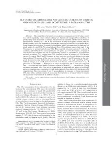
The structure relations in a special A∞ -bialgebra (H, d, mi , Δj )i,j≥2 easily follow from the following two observations: (1) if θ, η ∈ M, then θ • η = 0 whenever the projection of θ or η to M0 ⊕ M1 is zero; (2) each nonzero component in the projections of θ and η is represented by a horizontal, vertical or zero-length arrow. By (1), each component of dω • dω is a “transgression” represented by a “2-step” path of arrows from the horizontal axis M1,∗ to the vertical axis M∗,1 and by (2), each such 2-step path follows the edges of a (possibly degenerate) rectangle positioned with one of its vertices at (1, 1). Now relations involving d arise from degenerate rectangles since arrows of length zero represent components in the (co)extensions of d. Hence d interacts only with mi or Δj and the relations involving d are exactly the classical quadratic relations in an A∞ -(co)algebra. On the other hand, relations involving mi and Δj arise from nondegenerate rectangles since mi and Δj are represented by the arrows (i, 1) → (1, 1) and (1, 1) → (1, j). While the two-step path (i, 1) → (1, 1) → 449

  6

m3 m2 (1 ⊗ m2 ) 



m2 m2





m2 (m2 ⊗ 1) m3

+



6

[Δ2 ]

6

[Δ2 Δ2 ]



[Δ2 Δ2 Δ2 ]

[m2 ] [m3 ] Fig. 4. Some low-order arrows in M.

(1, j) represents the (usual) composition Δj • mi , the two-step path (i, 1) → (i, j) → (1, j) represents ξ j (ei−2 ) • ζ i (ej−2 ). Thus, we obtain the relation Δj • mi = ξ j (ei−2 ) • ζ i (ej−2 ). For example, by setting i = j = 2 we obtain the classical bialgebra relation   m2 • [Δ2 Δ2 ] . Δ2 • m2 = m2 And for (i, j) = (3, 2), we obtain Δ2 • m3 =



m3 m2 (1 ⊗ m2 )



 +

m2 (m2 ⊗ 1) m3

 • [Δ2 Δ2 Δ2 ]

(see Fig. 4). We summarize the discussion above in our main theorem. Theorem 1. Let (H, d, mi , Δj )i,j≥2 be a special A∞ -bialgebra. Then (H, d, mi )i≥2 is an A∞ -algebra, (H, d, Δj )j≥2 is an A∞ -coalgebra and for all i, j ≥ 2, Δj • mi = ξ j (ei−2 ) • ζ i (ej−2 ). REFERENCES 1. J. F. Adams, “Infinite loop spaces,” Ann. Math. Stud., 90 (1978). 2. V. K. A. M. Gugenheim, “On a perturbation theory for the homology of the loop-space,” J. Pure Appl. Algebra, 25, No. 2, 197–205 (1982). 3. T. Kadeishvili, “On the homology theory of fiber spaces,” Russian Math. Surveys, 35, 131–138 (1980). 4. M. Markl, S. Shnider, and J. Stasheff, “Operads in algebra, topology and physics,” Math. Surveys and Monogr., 96 (2002). 5. S. Saneblidze and R. Umble, “Diagonals on the permutahedra, multiplihedra and associahedra,” Homology Homotopy Appl., 6, No. 1, 363–411 (2004) (electronic). 6. S. Saneblidze and R. Umble, “The biderivative and A∞ -bialgebras,” Homology Homotopy Appl., 7(2005), No. 2, 161–177. 7. S. Saneblidze and R. Umble, “Matrons and the category of A∞ -bialgebras,” (in preparation). 8. B. Shoikhet, The CROCs, Non-commutative Deformations, and (Co)associative Bialgebras, preprint, math. QA/0306143. R. Umble Millersville University of Pennsylvania 450