CALVIN, The University of Edinburgh, Scotland (UK). {michele.volpi,vittorio.ferrari}@ed.ac.uk. AbstractâIn this work we address the problem of semantic.
Structured prediction for urban scene semantic segmentation with geographic context Michele Volpi, Vittorio Ferrari CALVIN, The University of Edinburgh, Scotland (UK) {michele.volpi,vittorio.ferrari}@ed.ac.uk Abstract—In this work we address the problem of semantic segmentation of urban remote sensing images into land cover maps. We propose to tackle this task by learning the geographic context of classes and use it to favor or discourage certain spatial configuration of label assignments. For this reason, we learn from training data two spatial priors enforcing different key aspects of the geographical space: local co-occurrence and relative location of land cover classes. We propose to embed these geographic context potentials into a pairwise conditional random field (CRF) which models them jointly with unary potentials from a random forest (RF) classifier. We train the RF on a large set of descriptors which allow to properly account for the class appearance variations induced by the high spatial resolution. We evaluate our approach by an exhaustive experimental comparisons on a set of 20 QuickBird pansharpened multi-spectral images.
I.
I NTRODUCTION
Segmenting satellite and airborne images into land cover maps is a central challenge in remote sensing image analysis. Tailored and up-to-date maps of urban areas are central instruments for many applications, ranging from road network analysis to urban sprawl modeling. Nevertheless, semantic segmentation of urban scenes from very high spatial resolution images (VHR) is a particularly complex task. These scenes are usually characterized by metric to submetric geometric resolution with a relatively poor spectral information, in the range of 3 to 15 visible and near infrared channels. For this reason, direct spectral discrimination techniques are prone to fail. To partly alleviate this issue, recent literature examines the inclusion of features able to convey spatial information into the pixel classification process directly [1]. Although filtering the input signal favors nearby pixel to have the same label, the semantic context is not directly modeled. Markov Random Field (MRF) and Conditional Random Field (CRF) are structured prediction models that can naturally account for the relationships between outputs. Most of the applications in remote sensing rely on the use of generative MRF [2]. MRF allows to regularize the output of spectral classifiers enforcing simple label smoothness. Although accounting for the structured nature of the data, this prior assumption does not capture complex spatial dependencies between labels. To cope with this limitations, in this paper we exploit discriminative CRF to jointly model local class likelihoods (unary potentials) with samples’ semantic contextual interactions (geographic context pairwise potentials). The geographic context potentials play a central role in our pairwise CRF model. These terms can encode different priors about the spatial organization of classes directly learned from training data [3], [4], [5]. For this purpose, we introduce
two geographic context potentials for semantic segmentation of urban satellite data: local co-occurrence and relative location of land cover classes. Furthermore, we introduce a set of descriptors commonly employed in computer vision tasks [6], [7] able to capture the complex land cover class appearance variations induced by VHR images. Similarly to these works we also make use of superpixels, which allow us to reduce the number of samples involved into the modeling process while keeping an appropriate spatial support to extract complex features. A random forest (RF) classifier [8], [9] is then trained on this bank of descriptor to obtain class likelihoods for each superpixel, based on its appearance. We demonstrate the appropriateness of these models by comparing them to a standard RF classification. We employ a dataset we built from 20 multi-spectral QuickBird images acquired in 2002 over the city of Zurich (Switzerland). II.
C ONDITIONAL R ANDOM F IELDS WITH GEOGRAPHIC CONTEXT POTENTIALS
A CRF models the labeling of every superpixel in the image as the conditional distribution p(y|x, λ), where y = {yi }N i=1 is the labeling of N observed signals x = {xi }N i=1 and λ are the model parameters. The posterior is modeled over an irregular graph G = (V, E), where nodes i ∈ V represent superpixels and undirected edges (i, j) ∈ E connect adjacent nodes i and j. The set of neighbors of i is defined as Ni and includes all the superpixels sharing some boundary � with i. The � CRF models the posterior as p(y|x, λ) ∝ exp − E(y|x, λ) , with energy: X XX E(y|x, λ) = ϕi (xi , yi ) + λ φij (xi , xj , yi , yj ). i∈V
i∈V j∈Ni
(1) The terms ϕi (xi , yi ) and φij (xi , xj , yi , yj ) are respectively the unary and pairwise potentials, detailed in the next Sections. The parameter λ trades-off unary and pairwise terms. A. Unary potentials The role of the unary potential is to link the local observations made by an appearance classifier to class likelihoods. It brings into the CRF evidence about the most probable labeling for each node when considered in isolation. This is usually achieved by employing the probabilistic output of a discriminative classifier. In this work, we use a random forest classifier [8], [9]. In contrast to other classifiers outputting probabilities (e.g. SVM with Platt’s sigmoid fitting), RF naturally handle
[m]
[m]
240 160
20
80 0
0
−80 −160
−20
−240 −20
0
20
[m]
−240 −160 −80
0
80
160 240 [m]
−60
0
20
40
(a) [m]
[m]
240
60
160
40
80
20
0
0
−80
−20
−160
−40
−240
−60 −240 −160 −80
(b)
0
80
160 240 [m]
−40
−20
60 [m]
(c)
Fig. 1. (a) Example of superpixels obtained using the method of [10], (b) Local co-occurrence potential matrix and (c) relative location priors. Clockwise from upper left: small buildings given small buildings, small buildings given road, trees given trees, trees given roads.
multi-class problems, provide nonlinear class separations and can deal with many heterogeneous descriptors. The trees in the forest are composed by binary splits with thresholds trained by minimizing the entropy of the labels. We allow each tree to grow up to depth 15 or when a node √ contains only a single class. Each split function test D randomly sampled features, where D is the dimensionality of the descriptor set. Since a larger forest corresponds to less overfitting but more computations, we fixed its size to 100 trees as the accuracy over the validation set saturated. Once trained, the random forest provides for each test sample a label distribution pAPP (yi |xi ). We include this posterior in the CRF as ϕi (xi , yi ) = − log [pAPP (yi |xi )]. B. Geographic context pairwise potentials The main contribution of this paper resides in proposing different geographic context potentials for urban scene semantic segmentation. Remote sensing data is intimately related to the geographical space it represents. No matter the modality of the sensor or its ground sampling distance, a univocal relationship links each pixel to its the absolute geographical coordinates. We can consequently exploit these notions to favor or discourage particular labelings of the whole image. In the following, we present two geographic context pairwise potentials and the standard contrast sensitive smoothing [11]: Local co-occurrence (C OOC). This potential favors local arrangement of labels common in training images as φsij (xi , xj , yi , yj ) = − log [C(yi , yj )]. The co-occurrence matrix C is estimated from� training data as C(yi , yj ) �� = 1 s s s s , x ) < ρ + p y |y , d(x , x ) < ρ . p y |y , d(x COOC j i COOC i j i j j i 2 The function d(xsi , xsj ) returns the Euclidean distance between centers of superpixels i and j. For each node of a given class we count the label occurrences of all the nodes inside a circle of radius ρ. The optimal ρ (in meters, [m]) is selected on validation images. In our experiments, optimal local co-occurrence radius is 200[m]. We use conditionals instead of joint probabilities to reduce the bias induced by large and frequent classes. This potential avoids label associations rarely
observed in training images (e.g. a tree or a roof surrounded by water) while favoring common associations (e.g. buildings and roads) [3], [12]. This potential is shown in Fig. 1(a). Relative location prior (R ELOC). Compared to the local co-occurrence potential, the relative location prior encodes a finer spatial reasoning. Let emn = xsm − xsn denote the spatial displacement vectors between training nodes m and n. Then, the P potential is formulated as 1 φrij (xi , xj , yi , yj ) = − log[ |mn| mn gy 0 |y (emn , eij )], where the sum spans all the |mn| training displacement vectors linking nodes labeled as y to the ones labeled as y 0 . The function gy0 |y (emn , eij ) is a Gaussian kernel estimating the similarity between emn observed in training images and eij from the pairs of test superpixels in the given neighborhood Ni . Instead of forcing some spatially unordered co-occurrence of classes, the relative location prior is able to favor or discourage particular label associations based on the similarity to arrangement of nodes observed at training [4], [5]. Since the superpixelization method we use produces highly heterogeneous regions in both size and shape (see example in Fig. 1(a)), training the R ELOC from all the configurations of classes observed in training images ensures to some extent that relative displacements between neighbors in Ni at test time have been observed, no matter size and shape of superpixels. In contrast to natural images where the absolute ordering is important (e.g. sky is above grass) in remote sensing images this notion is less evident. However, such data show often spatially isotropic class co-occurrences. This pairwise energy is able to adaptively learn the range of such concentric interactions. An example of relative location prior are given in Fig. 1(c). Two nodes labeled as “small building” appear often at 5 to 20[m] distance, while the conditional density of “trees” given “road” occur at a much larger spatial scale, in the range of 40-100[m]. Contrast-sensitive smoothing (S MTH). This �energy is formulated as: φcij (xi , xj , yi , yj ) = 1 − h(xci , xcj ) [yi 6= yj ] [11]. The distance h(xci , xcj ) corresponds to a Chi-Squared distance between histograms computed over the binned spectral channels (see Section II-D). This potential favors neighboring nodes to share the same label if no spectral gradient separates them. The function [yi 6= yj ] returns 1 if yi 6= yj is true and 0 otherwise. In our experiments, we combine geographic context and contrast sensitive pairwise potentials into Eq. (1) to account for image contrasts as well. Weights λ are learned to minimize the error on training images. At test time, inference is performed using the average of the optimal parameters of training images. C. Inference We obtain the optimal image labeling y∗ by MAP estimation over the CRF by solving as y∗ = arg miny E(y|x, λ) [11]. Since we deal with a multi-class problem, the global optimum of the energy minimization in Eq. (1) cannot be found. However, a good approximation can be found using α-expansion moves [11], [13]. The α-expansion algorithm decomposes the multi-class problem into binary ones and iteratively solves each sub-problem until no decrease in the total energy is observed. Since our R ELOC potential may be not submodular, we solve the binary minimization using the QPBO solver of [13].
TABLE I.
No. 1 2 3 4 5 6 7 8 9 10 11 12
D ESCRIPTORS , DIMENSIONALITY AND TYPE . SP REFERS TO SUPERPIXEL , BB TO BOUNDING BOX .
Descriptor SP shape over its BB (resized to 8×8 pixels) SP area relative to the image area SP BB size relative to image size BB average coordinate Color (NIR-R) SIFT BOW Dilated color SIFT BOW Local Binary Pattern (NIR-R-G-B) BOW Dilated LBP BOW Oriented gradients (NIR-R-G-B) BOW Dilated OG BOW Max. response (NIR-R-G-B) BOW Dilated MR BOW NIR-R-G-B SP Mean + Standard deviation NDVI SP Mean + standard deviation Color histogram (21 bins per band) SP Color Thumbnail (resized to 8×8)
Dimension 8×8 1 2 2 300 300 300 300 300 300 300 300 8 2 84 8×8×4
Type Shape Shape Shape Location Texture Texture Texture Texture Texture Texture Texture Texture Spectral Spectral Spectral Spectral
D. Superpixels and descriptors The use of superpixels allows to trade-off the size of the modeling problem with the resolution of the predictions, while still providing good spatial support to extract powerful features. The Zurich dataset used in the experiments is composed by a total of 24M pixels. We reduce the total number of nodes to 113k by generating superpixels with the method of [10], as it is not limited to RGB data (see Fig. 1(a)). Before extracting descriptors spectral signals were normalized to unit `2 -norm. Table I summarizes the descriptors used. Each set of features has been designed to encode some peculiarity of the superpixel, such as appearance, shape or location in the image plane. The comprehensive set is similar to that in [6], [7]. In the case of descriptor no. 12, value of the pixels in the bounding box not belonging to the superpixel have been set to 0. Regarding bag-of-words (BOW) features (descriptors no. 5–8) filters responses are quantized in 300 visual words using the fast integer k-means as implemented in the vl feat library [14]. Each BOW representation of these filters encodes a particular aspect of the image, such as edge orientations, filter responses at multiple scales and local texture. We then normalize the resulting visual word histogram for each superpixel to unit `1 -norm. We also enriched the BOW representation by counting visual words occurrences 15 pixels around each superpixel (roughly 9[m]). This brings some basic spatial context into the estimation of the unary potentials as well. The dimensionality of the whole descriptor set is 2819. III.
E XPERIMENTS
We evaluate the geographic context CRF models on a dataset we prepared consisting by 20 multi-spectral pansharpened QuickBird images with a ground sample distance of 0.61[m]. The size of the images ranges from a minimum of 500×500 to a maximum of 1650 × 1650 pixels, with an average image size of 1000 × 1150 pixels. We manually annotated 9 different urban and peri-urban land cover classes: Roads, Small buildings, Trees, Grass, Commercial / Large buildings, Bare soil, Water, Railways and Swimming pools. We show an example in Fig. 2. To estimate the generalization ability of the system and to avoid spatial autocorrelation between training and testing instances, we adopted a leave-one-out strategy over images. We trained the model on 19 images and predicted class labels
on the held-out image. Free model parameters were selected over 3-fold cross validation over the 19 images. We compute accuracy measures over the aggregated predictions for the 20 held-out images. To evaluate the contribution of the increased modeling power brought by the geographic context and the advanced descriptors, we perform evaluations using spectral features alone (descriptors 9 and 10 in Tab. I) and the whole set separately. The CRF models are then compared by evaluating the different pairwise terms along with the two sets of unary potentials. We test 5 different combinations of pairwise potentials into the CRF: S MTH - contrast sensitive smoothing, C OOC - local co-occurrence, S MTH +C OOC - contrast sensitive + local co-occurrence, R ELOC - relative location prior, S MTH +R ELOC - contrast sensitive + relative location prior and and S MTH +C OOC +R ELOC - a weighted combination of the three potentials. As a baseline we employ the random forest classifier applied on superpixels independently, which is representative of many architectures common in the remote sensing literature [9]. This setting corresponds to use only unary potentials (U NARY in Tab. II). To provide a term of comparison with a modern computer vision technique, we compared to the Semantic Texton Forests (STF) by Shotton et al. [15]1 . For STF, we report accuracies using unary terms and a contrast sensitive pairwise CRF. IV.
R ESULTS AND DISCUSSION
Table II reports accuracy measures of the tested urban semantic segmentation task. We evaluate the different CRF models in terms of per-class producer’s accuracy, its average (PR, corresponding to the mean average class accuracy) and user’s accuracy averaged over classes (US). These measures are derived from the aggregated error matrix of the 20 heldout images The benefits of modeling the image context with a CRF are clear. While employing only a contrast sensitive smoothing (S MTH) may slightly improve the accuracy, the largest and most significant gains over the RF model are observed when adopting the geographic context pairwise potentials. On the one hand, the local co-occurrence potentials improve the pooled user’s accuracy by 6.10 and 6.11 US points (C OOC and S MTH +C OOC) employing only the spectral descriptors and by 2.68 US points when employing all descriptors (S MTH +C OOC). Using local co-occurrence potentials increases the confidence of the model by reducing false positives, but without necessarily improving the detection accuracy. An example is given in Fig. 2 for S MTH +C OOC, where the false detections of water on shadowed areas are almost completely removed by the geographic context potentials. On the other hand, the relative location prior does improve significantly the PR score, by 11.69 points when using only spectral descriptors and by 6.85 points when using all descriptors (S MTH +R ELOC in both cases). In this case, the detection accuracy is increased, but at the price of more false positives. Figure 2 S MTH +R ELOC shows the increased detection accuracy in particular for rare classes. The inclusion of the contrast sensitive terms further refines the accuracy 1 We modified and adapted for our purpose a MATLAB implementation at https://github.com/akanazawa/Semantic-texton-forests
R ESULTS FOR THE URBAN SEMANTIC SEGMENTATION OF Z URICH . B OLD NUMBERS REFER TO HIGHEST SCORES (± 0.01), WHILE ITALIC TO SECOND AND THIRD HIGHEST ONES . E NTRIES ARE COMPUTED OVER THE AGGREGATED ERROR MATRIX FROM THE 20 HELD - OUT IMAGE PREDICTIONS .
TABLE II.
Spectral descriptors only Model U NARY S MTH C OOC R ELOC S MTH +C OOC S MTH +R ELOC S MTH +C OOC +R ELOC
US 69.43 69.73 75.53 71.35 75.54 68.25 73.68
PR 65.00 65.18 65.95 75.57 66.09 76.69 74.55
Roads Build. Trees Grass Comm.
Whole set of descriptors
Soil
Water Rails
74.09 91.16 74.87 24.13 55.02 92.70 74.43 91.30 75.13 24.06 55.39 93.03 81.88 93.12 76.36 19.91 59.55 95.22 78.99 92.35 80.04 49.13 77.55 97.13 81.87 93.12 76.41 20.25 59.55 95.24 76.86 92.10 80.86 58.76 80.85 97.32 82.69 92.81 77.91 47.20 77.41 97.62 Semantic texton forest unary only S TF 66.54 71.72 74.61 65.91 93.84 71.32 44.85 77.82 95.59
Image
Roads
79.39 79.86 77.24 69.59 78.12 57.49 67.72
GT
RF SPE
Small buildings
Trees
5.64 5.40 0.58 43.10 0.58 53.96 34.97
Pools
88.02 88.02 89.66 92.27 89.66 92.03 92.65
US 75.86 76.05 78.31 71.39 78.54 72.50 73.39
PR 71.11 71.16 70.95 77.25 70.98 77.96 74.89
84.74 94.04 83.49 84.81 94.17 83.58 89.07 94.70 83.60 85.41 94.14 85.85 88.91 94.74 83.14 85.95 94.58 85.62 88.28 94.43 84.86 Semantic texton 26.75 94.78 69.01 72.16 76.21 71.68 95.80 68.90
S MTH +C OOC SPE S MTH +R ELOC SPE
Grass
Roads Build. Trees Grass Comm.
Comm. building
Bare soil
87.08 87.40 83.26 76.96 83.88 77.48 78.63
RF WS
Water
Soil
34.08 68.24 34.04 68.65 38.93 71.63 47.65 78.24 38.88 71.85 48.72 78.38 44.83 79.00 forest CRF 44.39 77.80
S MTH +C OOC WS
Railways
Water Rails
Pools
92.95 93.09 93.46 95.80 93.46 95.72 96.24
78.60 78.60 74.82 85.44 74.82 89.39 83.48
16.77 16.07 9.07 45.72 9.18 45.83 24.30
95.64 24.56 94.48
S MTH +R ELOC WS
Swimming pools
Fig. 2. Original false color NIR-R-G image and associated ground truth annotations (GT) along land cover maps for spectral descriptors only (SPE) and for the whole set of descriptors (WS). Maps from random forests (RF) are compared to conditional random fields (CRF). Best viewed in color.
scores. The S MTH +C OOC +R ELOC models perform in a more balanced way on both descriptor sets with respect to US and PR scores. The CRF models relying on the geographic context potentials outperform the S TF [15] in both US and PR scores. It appears clearly that structured output models improve significantly the classification of independent superpixels (U NARY). Simple contrast sensitive smoothing (S MTH) is outperformed by considering explicitly the geographic context of classes. In addition, exploiting complex descriptors globally ameliorates the per-class accuracy measures, even if peak values for some classes may decrease. The segmentation examples shown in Fig. 2 confirm these observations. V.
C ONCLUSIONS
In this paper we proposed and assessed the suitability of two geographic context potentials terms into a conditional random field (CRF) for urban semantic segmentation. These potentials allow to model the spatial dependency of classes in a much more finer manner than by simple contrast sensitive smoothing. Moreover, we introduced a set of descriptors commonly employed in computer vision tasks which allow to increase the accuracy of the obtained land cover maps. As illustrated in the experiments their coupled use significantly outperforms standard architectures. The proposed CRF models are revealed to be very powerful for highly structured data such as remote sensing images of urban areas.
[2]
[3]
[4]
[5] [6]
[7]
[8] [9]
[10] [11]
[12]
ACKNOWLEDGMENTS
[13]
This work was partly funded by Swiss National Science Foundation grant No. P2LAP2 148432 (http://p3.snf.ch/project-148432).
[14]
[15]
R EFERENCES [1]
M. Fauvel, Y. Tarabalka, J. A. Benediktsson, J. Chanussot, and J. C. Tilton, “Advances in spectral-spatial classification of hyperspectral images,” Proc. IEEE, vol. 101, no. 3, pp. 652–675, 2013.
G. Moser, S. B. Serpico, and J. A. Benediktsson, “Land-cover mapping by markov modeling of spatial-contextual information in very-highresolution remote sensing images,” Proc. IEEE, vol. 101, no. 3, pp. 631–651, 2013. A. Rabinovich, A. Vedaldi, G. Galleguillos, E. Wiewiora, and S. Belongie, “Objects in context,” in IEEE ICCV, Rio de Janeiro (Brasil), 2007. S. Gould, J. Rodgers, D. Cohen, G. Elidan, and D. Koller, “Multi-class segmentation with relative location prior,” Int. J. Comp. Vision, vol. 80, no. 3, pp. 300–316, 2008. M. Guillaumin, L. Van Gool, and V. Ferrari, “Fast energy minimization using learned state filters,” in IEEE CVPR, Portland (USA), 2013. T. Malisiewicz and A. A. Efros, “Recognition by association via learning per-exemplar distances,” in IEEE CVPR, Anchorage (USA), 2008. J. Tighe and S. Lazebnik, “Superparsing: Scalable nonparametric image parsing with superpixels,” Int. J. Comp. Vision, vol. 101, no. 2, pp. 329– 349, 2013. L. Breiman, “Random forests,” Machine Learning, vol. 45, no. 1, pp. 5–32, 2001. V. F. Rodriguez-Galiano, B. Ghimire, J. Rogan, M. Chica-Olmo, and J. P. Rigol-Sanchez, “An assessment of the effectiveness of a random forest classifier for land-cover classification,” ISPRS J. Photo. Remote Sens., no. 67, pp. 93–104, 2012. P. Felzenswalb and D. Huttenlocher, “Efficient graph-based image segmentation,” Int. J. Comp. Vision, vol. 59, no. 2, pp. 167–181, 2004. Y. Boykov, O. Veksler, and R. Zabih, “Fast approximate energy minimization via graph cuts,” IEEE Trans. Pattern Anal. Mach. Intell, vol. 23, no. 11, pp. 1222–1239, 2001. L. Ladick´y, C. Russell, P. Kohli, and P. Torr, “Graph cut based inference with co-occurrence statistics,” in ECCV 2010, Hersonissos (Greece), 2010. V. Kolmogorov and C. Rother, “Minimizing non-submodular functions with graph cuts – a review,” IEEE Trans. Pattern Anal. Mach. Intell, vol. 29, no. 7, pp. 1274–1270, 2007. A. Vedaldi and B. Fulkerson, “VLFeat: An open and portable library of computer vision algorithms,” in ACM Multimedia, 2010, pp. 1469– 1472. J. Shotton, M. Johnson, and R. Cipolla, “Semantic texton forests for image categorization and segmentation,” in IEEE CVPR, Anchorage (USA), 2008.